Abstract
Air sampling for 12 h diurnal and nocturnal periods was conducted at two monitoring sites with different characteristics in Jambi City, Sumatra Island, Indonesia. The sampling was done at a roadside site and a riverside site from 2–9 August, and from 7–13 August in 2019, respectively. A cascade air sampler was used to obtain information on the status, characteristics and behavior of airborne particles with a particular focus on the ultrafine fraction (PM0.1). The number of light vehicles was best correlated with most PM size categories, while those of heavy vehicles and motorcycles with the 0.5–1 μm and with >10 μm for the nocturnal period, respectively. These findings suggest that there is a positive influence of traffic amount on the PM concentration. Using carbonaceous parameters related to heavy-vehicle emissions such as EC and soot-EC, HV emission was confirmed to account for the PM0.1 fraction more clearly in the roadside environment. The correlation between OC/EC and EC for 0.5–1 μm particles indicated that biomass burning has an influence on both in the diurnal period. A possible transboundary influence was shown as a shift in the PM0.1 fraction characteristic from “urban” to “biomass burning”.
1. Introduction
Ambient size-classified particulate matter (PMs) down to nano-size (dp ≤ 0.1 µm or 100 nm) range has become an important issue in the atmospheric scientific communities in the past decade [1,2,3]. Particulate pollution has contributed to the deterioration in air quality in many countries [2,4,5,6]. The effects of ambient particles can be detrimental to the overall global climate, visibility, and public health [7,8,9]. Substantial evidence from medical research suggests that finer particles, especially ultrafine particles (UFPs), or PM0.1, can pass into the bloodstream in the human body and then exert a variety of health effects [10,11]. In metropolitan areas, land transportation is an important source of UFP emissions [12]. Diesel and gasoline engines are the major source of UFPs in megacities [13]. As reported by Kumar et al. (2013), forest fires released higher levels of PM0.1 particles into the atmosphere than car engines, with sizes of approximately 120 nm a fresh aerosol plume [12].
Indonesia is one of the large contributors to atmospheric pollution due to extensive open biomass burning in the dry season in the past decade [14,15]. The dry season in Indonesia, which commonly occurs from June to October, causes large numbers of peatland/forest fires annually in several provinces including Jambi City in Sumatra Island, Indonesia [16,17]. As reported by the World Bank Group (2016), around 123,000 hectares of forest in Jambi had burned between June and October 2015 [18]. These fires account for 5 percent of the total area of forest fires in Indonesia. A great amount of smoke haze is emitted into the atmosphere in this area. Moreover, due to the influence of meteorological conditions, i.e., wind speed and direction, smoke haze in Jambi is not only a local problem but also contributes to transboundary haze pollution. Such pollution can be transported to neighboring provinces and neighboring countries such as Malaysia, Singapore, southern Thailand, and, of course, it has an impact on the multisector aspect of activities in those countries [14,19,20,21,22,23]. As a result, the origin of the worst air pollution in Jambi City is not only from transportation sources but also from biomass burning.
The main efforts made to understand Indonesia’s air quality have focused on the status of coarse (PM10, and TSP) and fine (PM2.5) particles [16,24]. Several studies based on remote sensing, monitoring and modelling techniques have revealed that aerosol plumes during smoke-haze incidents exceeded the national standard for Indonesia, which actually has a very high value compared to the World Health Organization (WHO) standard [21,25]. As reported by Handika et al. (2019), the PM10 concentration in roadsides is higher than the limit standard set by WHO for both weekdays and weekends [26]. Because of this, most studies have focused on coarse and fine particles. Studies dealing with smaller size particles as UFPs in Indonesia were still limited [27].
In the present study, therefore, in order to comprehensively understand the present status, characteristics and emission sources of PMs, including ultrafine particles in Indonesia, size-segregate airborne particles were collected in the City of Jambi as a typical provincial city in Sumatra Island. To accomplish this, air samples were collected for 12 h diurnal and nocturnal periods at two monitoring sites with different characteristics (a road side and a river side) from 2–13 August 2019, using a cascade air sampler that can collect size-segregated PMs down to the UFP range. Diurnal and nocturnal behaviors of the PM characteristics as particle mass and particle-bound carbonaceous components are discussed in relation to the influence of local sources and meteorological conditions, such as the thickness of the mixing layer. The number of the variety of vehicles observed in the roadside environment was correlated with PM mass and parameters for the carbonaceous components. The transboundary influence of peatland fires was also discussed by taking into account the correlation between the PM parameters and the number of hotspots, as determined by MODIS and backward air mass trajectory (HYSPLIT4). The influence of biomass burning and traffic emission was also examined based on OC/EC vs. EC correlations for PM0.1 and PM0.5–1 in comparison with those for urban and near-peatland fire areas.
2. Methodology
2.1. Sampling Site
2.1.1. Site for the Monitoring Campaign
The monitoring campaign was conducted at two different sites in Jambi City (see Figure 1). Jambi City had a total population of around 604,700 in 2019 and is located in Jambi Province within the territory of the Muaro Jambi Regency. This region has an average monthly temperature and humidity range from 27.1 to 28.2 °C and from 50 to 96%, respectively, which may affect the agglomeration of UFP [28,29]. Jambi City is 10 to 60 m above sea level. This district covers 4659 km2 (9.29 percent of Jambi Province), in which around 44 industries, including the agricultural and forest products industry (palm oil and rubber industry), mining, metals, machinery, and the chemical industry, are situated within the city. All of these industries are located southeast (SE), south (S), and southwest (SW) of both sampling sites. Since peatland areas are located in the vicinity of Jambi City and other districts in Jambi Province, the area of study has been faced with annual forest fires since the 1990s [30]. The total burned area in the Jambi Province has increased significantly from 2017 to 2019 after a dramatic decrease in 2016 [31].
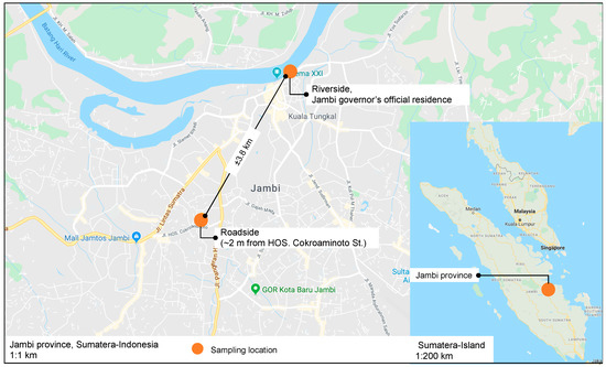
Figure 1.
Sampling site at the roadside and riverside in Jambi City, Indonesia.
The monitoring sites were selected because they are exposed to different sources of PMs, particularly ultrafine particles. Selected sites were located in areas with different characteristics, or, a roadside (RS) and a riverside (RV). These sites were selected to evaluate the environment, not only at one site, but at two or more locations so as to collect information concerning the general environment. The RS site was located beside HOS. Cokromaminoto Street, Suka Karya, Kota Baru District (1°37′04.6″ S 103°36′01.2” E). This street is one of the busiest roads in Jambi City in terms of traffic, especially by heavy vehicles (HV) such as trucks, which would represent important emission sources. The RV site was located in the rooftop of the official offices of the Governor of Jambi (1°35′17.5” S 103°37′05.1” E) near Raden Pamuk Street (~30 m) and the Batanghari River (~115 m), the longest river in Jambi Province. It serves as the main transportation route between the Tanjung Jabung Timur district. It is located on the other side of the river, and the central area of Jambi City by citizens who attend school, work in offices, markets and tourists are also present [32]. Although the river used to be of significant importance for boat transportation both by citizens and fishermen, the volume of traffic on the river has drastically decreased since the completion of a bridge over the river in 2015 [33].
2.1.2. Reference Site for Biomass Burning
For reference, data were collected regarding emissions from peatland fires. This was done on 24 August 2019 at a site located in a peatland area where fires frequently occur. The sampling site is located at 1°35′43” S 103°49′46” E in Arang-arang village, Kumpeh Ulu subdistrict, Muaro Jambi regency. Kumpeh Ulu subdistrict is the fifth largest area in the Muaro Jambi regency (386.65 km2 or 7.34% of the Muaro Jambi area) (BPS Muaro Jambi, 2019). The site is surrounded by palm oil plantations that are located some distance from main streets. The details of the sampling site are shown in Figure S1.
2.2. Air Sampling
PMs were collected by using a cascade air sampler developed by Furuuchi et al. (2010) (referred to herein as ANS), which is capable of classifying PMs down to the nano-size range (PM0.1) [34]. This sampler consists of six stages for size-classified particles, or, PM>10, PM10–2.5, PM2.5–1, PM1–0.5, PM0.5–0.1, and PM0.1, respectively, in which the original cutoff size of the last stage (0.07 μm) was adjusted to 0.1 μm [35]. Quartz fibrous filters (QFF) (2500 QAT-UP, Pall Corp., New York, NY, USA) of ∅ 55 mm were used for the sampling in the first 4 stages (PM>10, PM10–2.5, PM2.5–1, PM1–0.5) and the last stage (PM0.1). The filters were pre-baked at 350 °C in an oven for 1 h following the PM2.5 manual from the Ministry of Environment, Japan [36], and then conditioned at 21.5 ± 1.5 °C and 35 ± 5% RH in a PM2.5 weighing chamber (PWS-PM2.5, Tokyo Dylec Corp., Tokyo, Japan) before weighing by an electric micro-balance (Sartorius Cubis MSU2.7S-000-DF, MD = 1 μg). An inertial filter (IF) consisting of webbed stainless-steel fibers (average fiber diameter df = 9.8 μm, Nippon Seisen Co. Ltd., Osaka, Japan, felt type, SUS-316) in a cartridge nozzle of ∅ 5.25 mm [34,37] was used for the fifth stage to separate the PM0.1 fraction. Aluminum foil was used to cover each filter before storing it in a polyethylene bag. Filters were transported between Kanazawa, Japan, and the sampling sites in Jambi, Indonesia. All of the filters were accompanied by several blank filters to account for possible contamination during their transport.
The air sampling was conducted for 7 continuous days from 2 August to 9 August at the RS site and for 6 continuous days at the RV site from 7 August to 13 August 2019. In order to collect information concerning diurnal and nocturnal behavior, the air sampling was conducted for 11–12 h in each time range, or, 6:00 a.m.–6:00 p.m. and 6:00 p.m.–6:00 a.m.. Conditions for the air sampling are summarized in Table S1.
2.3. Traffic Density
The number of vehicles was manually counted by volunteers at the RS site by using handheld counters during the two different time periods, or, the day time (from 6:00 a.m. to 6:00 p.m.) and night time (from 6:00 p.m. to 6:00 a.m.), simultaneously with the air sampling. The vehicles were classified into three categories as motorcycles (MC), light vehicles or LV (cars and taxis) and HV (trucks) and are listed in Table S2.
2.4. Thermal-Optical Carbon Analysis
Carbonaceous components as organic carbon (OC) and elemental carbon (EC) of samples on all impactor stages were evaluated by using a thermal/optical carbon analyzer (Carbon Aerosol Analyzer, Sunset Laboratory, Tigard, OR, USA), following the IMPROVE-TOR protocol [38,39,40]. Samples collected on the IF stage were not analyzed since they are not applicable to the thermal/optical analysis. A QFF sample was punched to produce a 10 × 15 mm area and the resulting sample was placed in the carbon analyzer for analysis. The sample was then heated inside the analyzer at temperatures of 120, 250, 450 and 550 °C to produce four different OC fractions, i.e., OC1, OC2, OC3 and OC4, respectively, in a 100% helium atmosphere and three different EC fractions, i.e., EC1, EC2 and EC3 at 550, 700 and 800 °C, respectively, in a mixture of 2% oxygen and 98% helium. Then followed the addition of O2 to the experimental atmosphere, thus, pyrolysis organic carbon (pyOC) can be determined after the reflected laser light reaches its original intensity. The EC fraction was divided into char-EC and soot-EC [38,41]. Char-EC is EC1-pyOC, while soot-EC is EC2+EC3. The total OC is defined as OC1+OC2+OC3+OC4+pyOC, whereas the total EC is EC1+EC2+EC3-pyOC. Concerning quality assurance and quality control (QA/QC), a reference standard, i.e., sucrose (C12H22O11) (196-00015, Sucrose, Wako Pure Chemical Industries, Ltd., Osaka, Japan) and blank filters (n = 4) were used for the calibration. The repeatability of the analyses of the particle spots deposited on the filters was acceptable, with a CV less than 3.2% for OC and 7.9% for EC. The minimum detection limits (MDL) for OC and EC based on the evaluation of the travel blanks were 0.57 and 0.00 μg/cm2, respectively. These values were somewhat smaller than the minimum value of samples in the present study, or, 5.41 and 1.38 μg/cm2, respectively, for OC and EC.
2.5. Backward Trajectory and Hotspots
Backward trajectories of air mass movement in 72 h arriving at the sampling sites were determined at 500 m above ground level (a.g.l.) by using the Hybrid Single-Particle Lagrangian Integrated Trajectory Model version 4 (HYSPLIT4) [42], following previous reports on backward trajectories in Indonesia [27,43]. This is a sort of compromise between the limitation in the model and the data observed at the ground surface [44].
The data for hotspots, a marker of open biomass burning evaluated from Moderate Resolution Imaging Spectroradiometer (MODIS) satellite remote sensing imagery, was used to discuss the level of open burning a 1 km × 1 km resolution [45] for a medium and high confidence level. The number of MODIS hotspots provided by NASA was counted and used to determine the relation between the number of hotspots and characteristics of PMs.
3. Results and Discussion
3.1. Particle Mass Concentration
3.1.1. PM Mass Concentration
The mass concentrations of PMs in each size range averaged for the diurnal (D) and nocturnal (N) periods are shown in Figure 2a,b, respectively, at the roadside (RS) and the riverside (RV) sites. The 12 h mean, minimum and maximum values are summarized in Table 1. The values for PM size categories, or, PM0.1/1/2.5/10 and total suspended particulate (TSP), are also listed in Table 1. The diurnal minimum, mean, and maximum concentrations of PM0.1 at the RS site were 11.7, 14.0 ± 1.6 and 16.2 µg/m3, while the corresponding nocturnal levels increased to 21.5, 24.7 ± 2.9, and 29.2 µg/m3, respectively. These values are somewhat comparable to a case in another city in Indonesia (see Table S3), although they were slightly less in the diurnal period and about two times larger in the nocturnal period [27]. The present diurnal average for the PM0.1 fraction in the roadside environment (19.4 μg/m3) was higher than values reported for other cities in Southeast Asia (SEA), as listed in Table S3. Diurnal and nocturnal average fractions of each size range of particles were compared between the RS and RV sites, and the results are shown in Figure 3. The percentage of PM0.1 fraction was around 17~19% larger than that for other countries [46,47]. However, it was not significantly different in terms of the location and time period. The average levels of PM2.5 and PM10 at all sites consistently exceeded the WHO guidelines (25 and 50 μg/m3, respectively) for 24 h. However, the daily average PM2.5 value at the RV site (53 ± 13.9 μg/m3) was still below the national air quality standards (the Indonesian Government No. 22/2021; 55 and 75 μg/m3 for PM2.5 and PM10, respectively) [48]. These results suggest that the PM mass concentration and its behavior were rather comparable and consistent with other locations in SEA.
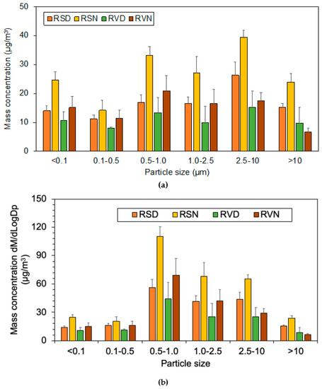
Figure 2.
Average of mass (a) direct (b) dM/dLogDp concentration of each size PMs in RS and RV at diurnal and nocturnal in Jambi City.

Table 1.
The daily mean, minimum, and maximum of size-segregated PMs in roadside and riverside, Jambi City, Indonesia.
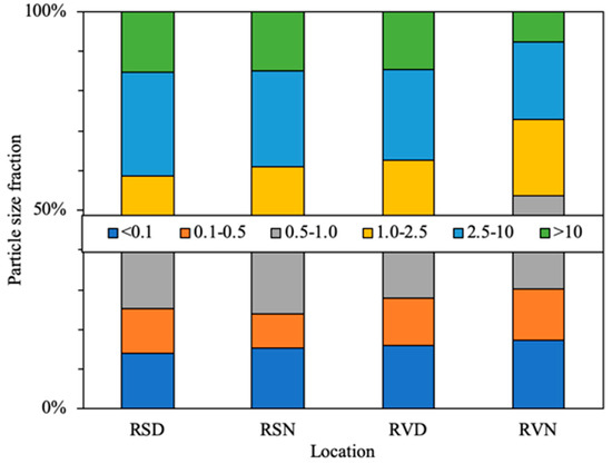
Figure 3.
Size-segregated particles fraction of the airborne particles in RS and RV at diurnal and nocturnal in Jambi City.
3.1.2. Influence of Location and Time Period on PM Concentration
As a reason for the differences in the PM concentration with location and time period, the amount of traffic is an important factor. To confirm this, the correlation between the concentration of each size range and grouped PMs (PM0.1/1/2.5/10 and TSP) at the RS site and the number of each type of vehicles was examined for the diurnal and nocturnal periods (see Table S2). The calculated correlation factors are shown in Table S4. The PM mass concentration (PMC) was correlated with the number of MC, LV, HV and total vehicles (TV) observed in each time period. The LV number that shared 34.4% of the diurnal total and 29.8% of the nocturnal total was found to show the best correlation for most of the size categories. To the contrary, the HV number was correlated best for the nocturnal 0.5–1 μm (R2 = 0.45). The MC number was the largest contribution to the coarse fraction (>10 μm) in both the diurnal (R2 = 0.48) and nocturnal (R2 = 0.65) periods. Although the correlation was moderate, the amount of traffic had a positive influence on the PM concentration. This, therefore, can explain the average PM level at the RS site, which was nearly 50% larger than that at the RV site. This is because the RS site was located near the busiest street in Jambi City, while the RV site was located slightly more distant at the nearest street. However, the road traffic was the dominant source at both locations.
As shown in Figure 2 and Table 1, the PM level at both sites increased in the nocturnal period, except for the >10 μm range in the nocturnal period at the RV site. The nocturnal average TSP concentration at the RS site increased to 162% of the diurnal value. The maximum increase was found in the 0.5–1 μm fraction at 96%. To the contrary, there was a 53% decrease in the average total amount of traffic in the nocturnal period (see Table S2). However, a decrease in HV number was not so significant (~20%). As reported so far [49,50,51], such differences between the diurnal and nocturnal PM levels could also be affected by a change in the thickness of the mixing layer. By assuming that the PM2.5 emission is attributed only to the LV number, an average diurnal/nocturnal ratio of the thickness of a mixing layer can be estimated to be ~4, where the average diurnal/nocturnal ratios of PM2.5 and LV number at the RS site were 0.60 and 2.47, respectively. This is slightly smaller than other reported values [49,52,53]. Since there should be other emission sources, these numbers may be overestimates of the actual value. A moderate increase in the PM fraction of 2.5–10 μm and a slight decrease in the coarse fraction (>10 μm) in the nocturnal period at the RV site may be related to a drastic decrease in the amount of road traffic, e.g., as MC and LV.
3.2. Contribution of Local Emission Sources
3.2.1. Carbonaceous Parameters Sensitive to Vehicle Emission
In order to specify the carbonaceous parameters that are sensitive to the influence of vehicle emissions, correlation factors between the number of vehicles counted for each category, i.e., MC, LV, HV and TV, and carbonaceous parameters along with PMC, or, OC, EC, OC/EC, soot-EC, soot-EC/TC, soot-EC/PMC, (TC = OC + EC), were calculated for each size range of particles collected at the RS site. The results are summarized in Table S5. Diurnal EC and soot-EC-related parameters for the PM0.1 fraction appear to be well correlated with the number of HV (R2 = 0.52–0.82). Although it is not as clear as the diurnal period, a nocturnal correlation between soot-EC/TC and the HV number for PM0.1 exhibited the largest R2 (0.47). Nocturnal soot-EC and related parameters for PM1–2.5 were also fairly well correlated with the HV number (R2 = 0.60–0.66). Since, in the >10 μm size range, the concentration was much smaller than those of other sizes, rather large correlation factors, e.g., 0.65–0.78 for the nocturnal LV number, need to be carefully viewed. Although there were differences in the degree of correlation depending on the time period and particle size, the EC and soot-EC-related parameters especially for the PM0.1 fraction, therefore, appear to be suitable as indices for HV emissions. These tendencies are consistent with other results reported so far [54].
3.2.2. Behavior of Carbonaceous Components in Size-Fractionated Particles
Figure 4a–f shows the average values for the targeted carbonaceous parameters, or, OC, EC, OC/EC, soot-EC, soot-EC/TC and soot-EC/PMC, for each size range, time period and location. The average values for the parameters including those above are summarized in Table 2. For comparison, the values for the average mass ratio of the analyzed carbonaceous components to TC are shown in Figure 5. The EC and soot-EC, parameters which are largely related to HV vehicle emissions, were not as sensitive as the PM concentrations. However, the difference with respect to location was consistent with the expected amount of traffic. The values for these parameters, as well as other HV-related parameters such as soot-EC/TC and soot-EC/PMC, were larger or peaked mostly with respect to the PM0.1 fraction, regardless of the location or the time of collection. This suggests that HV emissions largely account for the PM0.1 fraction at the RS site, where the largest EC3 fraction appeared also at PM0.1 (see Figure 5). Larger EC and soot-EC for fractions >10 μm at the RS site compared to those at the RV site are reasonable, since a larger amount of traffic would be expected. A similar level of soot-EC/TC at the RS site may be partially attributed to tire wear that shares, e.g., 3% of the PM10 [55,56,57,58,59].
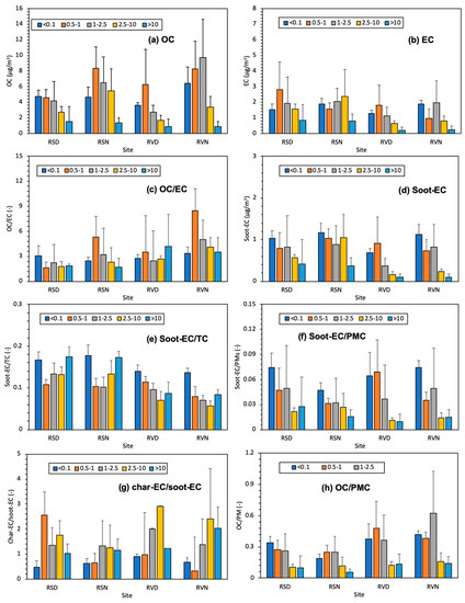
Figure 4.
Carbonaceous component and their ratios in RS and RV at diurnal and nocturnal in Jambi City: (a) OC, (b) EC, (c) OC/EC, (d) soot-EC, (e) soot-EC/TC, (f) soot-EC/PMC, (g) char-EC/soot-EC, (h) OC/PMC.
Table 2.
Particle-bound carbonaceous components and their ratio in Jambi City.
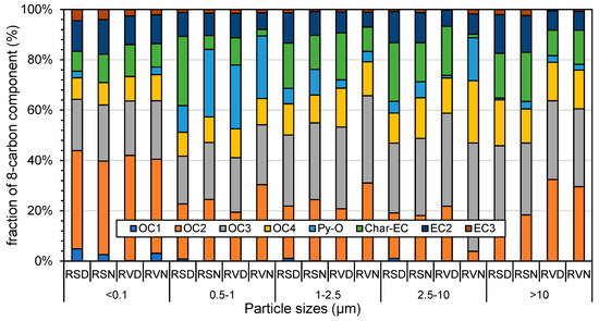
Figure 5.
Fraction 8 carbonaceous component for both RS and RV at diurnal and nocturnal.
Similar to findings reported in previous studies, the concentration of OC tends to peak at the 0.5–1 μm or 1–2.5 μm fraction except for the diurnal period at the RS site [2,3]. This is also clear for the OC/EC ratio, except for the RS site. As seen from Figure 5, such behavior can largely be attributed to larger fractions of pyOC and char-EC at both the RS and RV sites. Since these values and related parameters are generally accepted as indices of biomass burning, carbonaceous characteristics in the size range of 0.5–1 or 1–2.5 μm, they can be attributed to biomass burning or related emission sources [3,4]. The concentration of OC and OC/EC for the 0.5–1 and 1–2.5 μm fractions increased in the nocturnal period, where the OC/EC ratio was larger at the RV site, while EC and soot-EC were smaller, especially in the case of the >2.5 μm range. Such tendencies in the OC and related parameters may be explained by a larger amount of local biomass burning near the RV site. The larger average char-EC/soot-EC ratio for the 1–2.5 μm range at the RV site may also explain this.
3.3. Local and Transboundary Influence of Open Biomass Burning
Since biomass burning, especially from peatland fires, usually occurs in this region and surrounded provinces during the study period, it would be expected that this would have an influence on the level and characteristics of PMs, including PM0.1. A similar result was reported by Phairuang et al. (2019) in a study conducted in Chiang Mai, Thailand. The distribution of hotspots as an indicator of biomass burning and air mass trajectories at the sampling sites during the study periods are displayed in Figure S2. Many hotspots were distributed within Sumatra Island, particularly in the lower part of Jambi Province. Air-parcel trajectories were passing through this hotspot area before arriving at the sampling sites. Correlation factors between the daily base number of hotspots and the daily average study parameters were evaluated only for the southern Sumatra Island, as listed in Table S6. This is because most of the air mass arriving at the study sites was from the southern part of the island, and peatlands are located mainly on Sumatra Island. Although there were moderate correlations for PMC in size ranges of <0.1 and 0.1–0.5 μm at the RS site, it may not be reasonable to conclude that the influence of long-range transportation was responsible for this. This is because no meaningful correlations were found for the carbonaceous parameters for all size ranges. In addition, there was nearly no correlation at the RV site where the influence of transboundary PM pollution should be similar at both sites. These size ranges of particles are usually more sensitive to local sources, as discussed previously. This may be because the study term was not sufficiently long to permit a correlation to be observed, compared with studies involving longer periods [14,25]. Local and smaller spots that could not be detected from satellite data may also be a contributing factor.
In order to discuss both possible local and transboundary influences of biomass burning from a different point of view, a correlation between OC/EC and EC was plotted both for PM0.1 and PM0.5–1 at the RS and RV sites, following the previous report by Putri et al. (2021) [27]. The results are shown in Figure 6. Values for the PM0.5–1 fraction, at which OC and OC/EC frequently showed peaks (see Figure 4), are findings that are sensitive to biomass burning. Published data for the PM0.1 fraction obtained at several urban sites in Asian cities, i.e., Seoul, Korea (urban and roadside sites) [39,40], Saitama, Japan (urban site) [60], Hanoi, Vietnam (urban site) [1] and Bangkok, Thailand (urban site) [2] are also shown for reference. As reference values representing the influence of fresh biomass burning, the PM0.1 fractions from the peatland fire site are also shown in the upper-right side. Values from the above urban sites are likely to fall into a correlation with a narrow range of scattering, as shown by the dashed lines in Figure 6, which we refer to as “urban correlation”. Such a correlation may correspond to the dominant influence of fossil fuel burning as vehicle emissions. Although there were small differences with location and time period, the values for the PM0.1 fraction at the RS and RV sites were distributed along a similar correlation. This correlation slightly shifted to the biomass burning side, suggesting that biomass burning can have a slight influence on the background values. This is similar to a case in Chiang Mai during the forest fire season [2]. During the diurnal period at the RS site, the behaviors of the PM0.5–1 fraction were still similar to those of PM0.1. However, their behavior seems to reflect biomass burning, particularly during the nocturnal period, both at the RS and RV sites, where the values were largely scatted to the biomass burning side. Although the reason for such behavior is not clear at this time, it might be caused by local biomass burning, including local peatland fires. Further investigations will be needed to describe this, in which other information on heavy metals that could also be indices of the peatland fire should be added. However, it can be said that the correlation between OC/EC and EC for particle sizes representing typical emission sources may provide a useful perspective on the influence of emission from traffic and biomass burning.
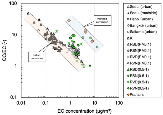
Figure 6.
OC/EC vs. EC in RS and RV and urban sites in several Asian countries.
4. Conclusions
An air sampling for 12 h diurnal and nocturnal periods at two monitoring sites with different characteristics was conducted in Jambi City, Sumatra Island, Indonesia, i.e., a roadside and a riverside, by using a cascade air sampler. Information on the status, characteristics and behavior of airborne particles with a particular focus on the PM0.1 fraction was collected. Local and transboundary influences were discussed in terms of the analysis of particle-bound carbonaceous components as well as the measurement of the amount of traffic passing through the study site and the analysis of hotspot distribution by MODIS and backward air mass trajectory by HYSPLIT4. Both the PM2.5 and PM10 fractions were confirmed to exceed the WHO and Indonesia National Air Quality Standard (NAQS) except PM2.5 at the riverside site. The number of LV was best correlated with most of the PM size categories. Contrarily, the number of HV was correlated best for the nocturnal 0.5–1 μm and the number of MC was best correlated with the coarse fraction (>10 μm) both in the diurnal and nocturnal periods, suggesting that the level of traffic clearly has a positive influence on the PM concentration. Using parameters related to HV emission such as EC and soot-EC, the predominant contribution to the HV emission was confirmed to be the PM0.1 fraction, especially in the roadside environment, where there was heavy traffic. Based on the correlation between OC/EC and EC for the size range of 0.5–1 μm, influences of biomass burning were shown to increase in the nocturnal period, probably because of local emission. A possible transboundary influence was shown as a shift in the PM0.1 fraction characteristic on this correlation from “urban” to “biomass burning”. In terms of size categories of carbonaceous components which are sensitive to each emission source, such as traffic and biomass burning, the influence of emission sources may be able to be fairly described based on the OC/EC vs. EC correlation. However, further investigations involving the use of other chemical components such as heavy metals and non-organic ions should be done in future study.
Supplementary Materials
The following are available online at https://www.mdpi.com/article/10.3390/app112110214/s1, Figure S1. Sampling site in roadside, riverside, and peatland area in Jambi city, Indonesia. Figure S2. Maps of hotspot and air mass trajectories during sampling time in Jambi city, Indonesia (a) roadside (2–9 August) and (b) riverside (7–13 August). Table S1. Sampling site, time, and its meteorological condition in Jambi city. Table S2. Daily total number of vehicles in roadside at diurnal and nocturnal in Jambi city. Table S3. The comparison of PM0.1 in Jambi city and other cities in Indonesia and South East Asian (SEA) countries. Table S4. Pearson correlation between types of vehicles and each particle sizes and PM categories. Table S5. Pearson correlation between types of vehicles, mass of PMs, and their carbonaceous component at diurnal and nocturnal. Table S6. Pearson correlation between the daily number of hotspots in southern part of Sumatera Island with daily mass of PMs, and their carbonaceous component at RS and RV sites.
Author Contributions
Conceptualization, M.A. and M.F.; investigation, R.A.H.; resources, M.A., R.M.P., M.F. and R.A.H.; data curation, M.A., M.H.; writing—original draft preparation, M.A.; writing—review and editing, W.P., P.T., M.H. and M.F.; visualization, M.A. and R.M.P.; supervision, M.H., M.F.; project administration, R.A.H. and M.H.; funding acquisition, M.H. and M.F. All authors have read and agreed to the published version of the manuscript.
Funding
This work has been supported by the Sumitomo Foundation (Kankyo Kenkyu Josei 2020-2021) and Japan Society for the Promotion of Science (JSPS) (KAKENHI 21H03618).
Institutional Review Board Statement
Not applicable.
Informed Consent Statement
Not applicable.
Data Availability Statement
Not applicable.
Acknowledgments
The authors gratefully acknowledge East Asia Nanoparticle Monitoring Network (EA-NanoNet) and students of the Department of Environmental Engineering, Jambi University, Indonesia, and of the Division of Environmental Design, Graduate School of Natural Science and Technology, Kanazawa University, Japan, for support and collaboration.
Conflicts of Interest
The authors declare no conflict of interest.
References
- Thuy, N.T.T.; Dung, N.T.; Sekiguchi, K.; Thuy, L.B.; Hien, N.T.T.; Yamaguchi, R. Mass Concentrations and Carbonaceous Compositions of PM0.1, PM2.5, and PM10 at Urban Locations of Hanoi, Vietnam. Aerosol Air Qual. Res. 2018, 18, 1591–1605. [Google Scholar] [CrossRef]
- Phairuang, W.; Suwattiga, P.; Chetiyanukornkul, T.; Hongtieab, S.; Limpaseni, W.; Ikemori, F.; Hata, M.; Furuuchi, M. The influence of the open burning of agricultural biomass and forest fires in Thailand on the carbonaceous components in size-fractionated particles. Environ. Pollut. 2019, 247, 238–247. [Google Scholar] [CrossRef]
- Phairuang, W.; Inerb, M.; Furuuchi, M.; Hata, M.; Tekasakul, S.; Tekasakul, P. Size-fractionated carbonaceous aerosols down to PM0.1 in southern Thailand: Local and long-range transport effects. Environ. Pollut. 2020, 260, 114031. [Google Scholar] [CrossRef]
- Fujii, Y.; Kawamoto, H.; Tohno, S.; Oda, M.; Iriana, W.; Lestari, P. Characteristics of carbonaceous aerosols emitted from peatland fire in Riau, Sumatra, Indonesia (2): Identification of organic compounds. Atmos. Environ. 2015, 110, 1–7. [Google Scholar] [CrossRef]
- Budisulistiorini, S.H.; Riva, M.; Williams, M.; Chen, J.; Itoh, M.; Surratt, J.D.; Kuwata, M. Light-Absorbing Brown Carbon Aerosol Constituents from Combustion of Indonesian Peat and Biomass. Environ. Sci. Technol. 2017, 51, 4415–4423. [Google Scholar] [CrossRef] [PubMed]
- Mannucci, P.M.; Franchini, M. Health Effects of Ambient Air Pollution in Developing Countries. Int. J. Environ. Res. Public Health 2017, 14, 1048. [Google Scholar] [CrossRef] [PubMed]
- Xing, Y.-F.; Xu, Y.-H.; Shi, M.-H.; Lian, Y.-X. The impact of PM2.5 on the human respiratory system. J. Thorac. Dis. 2016, 8, E69–E74. [Google Scholar] [CrossRef] [PubMed]
- Doherty, R.M.; Heal, M.R.; O’Connor, F.M. Climate change impacts on human health over Europe through its effect on air quality. Environ. Health 2017, 16, 118. [Google Scholar] [CrossRef]
- Manisalidis, I.; Stavropoulou, E.; Stavropoulos, A.; Bezirtzoglou, E. Environmental and Health Impacts of Air Pollution: A Review. Front. Public Health 2020, 8, 14. [Google Scholar] [CrossRef]
- Slezakova, K.; Morais, S.; Pereir, M.D.C. Atmospheric Nanoparticles and Their Impacts on Public Health. In Current Topics in Public Health; InTech Open: London, UK, 2013; Volume 10, pp. 5772–5775. [Google Scholar] [CrossRef]
- Schraufnagel, D.E. The health effects of ultrafine particles. Exp. Mol. Med. 2020, 52, 311–317. [Google Scholar] [CrossRef]
- Kumar, P.; Pirjola, L.; Ketzel, M.; Harrison, R.M. Nanoparticle emissions from 11 non-vehicle exhaust sources—A review. Atmos. Environ. 2013, 67, 252–277. [Google Scholar] [CrossRef]
- De Jesus, A.L.; Rahman, M.; Mazaheri, M.; Thompson, M.; Knibbs, L.; Jeong, C.; Evans, G.; Nei, W.; Ding, A.; Qiao, L.; et al. Ultrafine particles and PM2.5 in the air of cities around the world: Are they representative of each other? Environ. Int. 2019, 129, 118–135. [Google Scholar] [CrossRef] [PubMed]
- Kusumaningtyas, S.D.A.; Aldrian, E. Impact of the June 2013 Riau province Sumatera smoke haze event on regional air pollution. Environ. Res. Lett. 2016, 11, 075007. [Google Scholar] [CrossRef]
- Prasetyo, L.B.; Dharmawan, A.H.; Nasdian, F.T.; Ramdhoni, S. Historical Forest fire Occurrence Analysis in Jambi Province During the Period of 2000–2015: Its Distribution & Land Cover Trajectories. Procedia Environ. Sci. 2016, 33, 450–459. [Google Scholar] [CrossRef]
- Reddington, C.L.; Yoshioka, M.; Balasubramanian, R.; Ridley, D.; Toh, Y.Y.; Arnold, S.; Spracklen, D.V. Contribution of vegetation and peat fires to particulate air pollution in Southeast Asia. Environ. Res. Lett. 2014, 9, 1748. [Google Scholar] [CrossRef]
- Purnomo, H.; Shantiko, B.; Sitorus, S.; Gunawan, H.; Achdiawan, R.; Kartodihardjo, H.; Dewayani, A.A. Fire economy and actor network of forest and land fires in Indonesia. For. Policy Econ. 2017, 78, 21–31. [Google Scholar] [CrossRef]
- World Bank Group. The Cost of Fire an Economic Analysis of Indonesia’s 2015 Fire Crisis; World Bank Group: Jakarta, Indonesia, 2016. [Google Scholar]
- Forsyth, T. Public concerns about transboundary haze: A comparison of Indonesia, Singapore, and Malaysia. Glob. Environ. Chang. 2014, 25, 76–86. [Google Scholar] [CrossRef]
- Othman, J.; Sahani, M.; Mahmud, M.; Ahmad, K.S. Transboundary smoke haze pollution in Malaysia: Inpatient health impacts and economic valuation. Environ. Pollut. 2014, 189, 194–201. [Google Scholar] [CrossRef]
- Marlier, M.; DeFries, R.S.; Kim, P.S.; Koplitz, S.; Jacob, D.J.; Mickley, L.J.; Myers, S.S. Fire emissions and regional air quality impacts from fires in oil palm, timber, and logging concessions in Indonesia. Environ. Res. Lett. 2015, 10. [Google Scholar] [CrossRef]
- Kim, Y.; Knowles, S.; Manley, J.; Radoias, V. Long-run health consequences of air pollution: Evidence from Indonesia’s forest fires of 1997. Econ. Hum. Biol. 2017, 26, 186–198. [Google Scholar] [CrossRef] [PubMed]
- Kuwata, M.; Neelam-Naganathan, G.-G.; Miyakawa, T.; Khan, F.; Kozan, O.; Kawasaki, M.; Sumin, S.; Latif, M.T. Constraining the Emission of Particulate Matter from Indonesian Peatland Burning Using Continuous Observation Data. J. Geophys. Res. Atmos. 2018, 123, 9828–9842. [Google Scholar] [CrossRef]
- Kunii, O.; Kanagawa, S.; Yajima, I.; Hisamatsu, Y.; Yamamura, S.; Amagai, T.; Ismail, I.T.S. The 1997 Haze Disaster in Indonesia: Its Air Quality and Health Effects. Arch. Environ. Health Int. J. 2002, 57, 16–22. [Google Scholar] [CrossRef]
- Anwar, A.; Juneng, L.; Othman, M.R.; Latif, M.T. Correlation between hotspots and air quality in Pekanbaru, Riau, Indonesia in 2006–2007. Sains Malays. 2010, 39, 169–174. [Google Scholar]
- Handika, R.; Lestari, R.; Saputra, R. Comparing contributors and PM10 dispersion around Tugu Juang and in governor office area of Jambi City, Indonesia. IOP Conf. Series Earth Environ. Sci. 2019, 391, 1088–1755. [Google Scholar] [CrossRef]
- Putri, R.M.; Amin, M.; Suciari, T.F.; Faisal, M.A.F.; Auliani, R.; Ikemori, F.; Wada, M.; Hata, M.; Tekasakul, P.; Furuuchi, M. Site-specific variation in mass concentration and chemical components in ambient nanoparticles (PM0.1) in North Sumatra Province-Indonesia. Atmos. Pollut. Res. 2021, 12, 101062. [Google Scholar] [CrossRef]
- Badan Pusat Statistik (BPS-Statistics of Jambi). Jambi Province in Figure; BPS: Jambi, Indonesia, 2021. [Google Scholar]
- He, Y.; Gu, Z.; Lu, W.; Zhang, L.; Okuda, T.; Fujioka, K.; Luo, H.; Yu, C.W. Atmospheric humidity and particle charging state on agglomeration of aerosol particles. Atmos. Environ. 2019, 197, 141–149. [Google Scholar] [CrossRef]
- Dennis, R.A. A Review of Fire Projects in Indonesia, 1982–1998; CIFOR: Bogor, Indonesia, 1999; p. 105. [Google Scholar]
- Direktorat PKHL Kementrian Lingkungan Hidup Dan Kehutanan RI. Rekapitulasi Luas Kebakaran Hutan dan Lahan (Ha) Per Provinsi Di Indonesia Tahun 2016–2020; KLHK: Jakarta, Indonesia, 2020; Available online: sipongi.menlhk.go.id (accessed on 1 April 2021).
- Zarmaili, Z. Evaluasi Transportasi Sungai Di Kabupaten Tanjung Jabung Timur Provinsi Jambi. War. Penelit. Perhub. 2019, 27, 117. [Google Scholar] [CrossRef][Green Version]
- Nurmalia, W. Pemanfaatan Modal Sosial Sebagai Strategi Bertahan Hidup Komunitas Terdampak Pembangunan: Studi Penarik Ketek Terdampak Pembangunan Jembatan di Kecamatan Pelayangan Kota Jambi. Master’s Thesis, Universitas Andalas, West Sumatra, Indonesia, 2017. (In Bahasa). [Google Scholar]
- Furuuchi, M.; Eryu, K.; Nagura, M.; Hata, M.; Kato, T.; Tajima, N.; Sekiguchi, K.; Ehara, K.; Seto, T.; Otani, Y. Development and Performance Evaluation of Air Sampler with Inertial Filter for Nanoparticle Sampling. Aerosol Air Qual. Res. 2010, 10, 185–192. [Google Scholar] [CrossRef]
- Kumsanlas, N.; Piriyakarnsakul, S.; Sok, P.; Hongtieab, S.; Ikemori, F.; Szymanski, W.W.; Hata, M.; Otani, Y.; Furuuchi, M. A Cascade Air Sampler with Multi-nozzle Inertial Filters for PM0.1. Aerosol Air Qual. Res. 2019, 19, 1666–1677. [Google Scholar] [CrossRef]
- MOEJ (Ministry of Environment of Japan). Chapter 4. Carbonaceous Component Analysis Method 483 (Thermal Optical Reflectance Method). In Fine Particles (PM2.5) Component 484 Measurement Manual, 3rd ed.; 2019; Available online: https://www.env.go.jp/air/osen/pm/ca/manual.html (accessed on 17 August 2020). (In Japanese)
- Otani, Y.; Eryu, K.; Furuuchi, M.; Tajima, N.; Tekasakul, P. Inertial Classification of Nanoparticles with Fibrous Filters. Aerosol Air Qual. Res. 2007, 7, 343–352. [Google Scholar] [CrossRef]
- Han, Y.; Cao, J.; Chow, J.C.; Watson, J.; An, Z.; Jin, Z.; Fung, K.; Liu, S. Evaluation of the thermal/optical reflectance method for discrimination between char- and soot-EC. Chemosphere 2007, 69, 569–574. [Google Scholar] [CrossRef] [PubMed]
- Kim, K.H.; Sekiguchi, K.; Furuuchi, M.; Sakamoto, K. Seasonal variation of carbonaceous and ionic components in ultrafine and fine particles in an urban area of Japan. Atmos. Environ. 2011, 45, 1581–1590. [Google Scholar] [CrossRef]
- Kim, K.H.; Sekiguchi, K.; Kudo, S.; Sakamoto, K. Characteristics of Atmospheric Elemental Carbon (Char and Soot) in Ultrafine and Fine Particles in a Roadside Environment, Japan. Aerosol Air Qual. Res. 2011, 11, 1–12. [Google Scholar] [CrossRef]
- Han, Y.; Lee, S.-C.; Cao, J.; Ho, K.F.; An, Z. Spatial distribution and seasonal variation of char-EC and soot-EC in the atmosphere over China. Atmos. Environ. 2009, 43, 6066–6073. [Google Scholar] [CrossRef]
- Air Resource Laboratory (ALR). The Air Resource Laboratory (HYSPLIP 4). 2019. Available online: http://ready.arl.noaa.gov/HYSPLIT.php (accessed on 10 August 2019).
- Budiwati, T.; Setyawati, W.; Tanti, D.A. Chemical Characteristics of Rainwater in Sumatera, Indonesia, during 2001–2010. Int. J. Atmos. Sci. 2016, 2016, 1–11. [Google Scholar] [CrossRef]
- Murao, N. Air Quality Model—6. Trajectory Analysis. J. Soc. Atmos. Environ. Japan 2011, 46, A61–A67. [Google Scholar]
- FIRMS. 2019. Available online: https://firms.modaps.eosdis.nasa.gov/download/list.php (accessed on 15 August 2019).
- Hongtieab, S.; Yoshikawa, F.; Matsuki, A.; Zhao, T.; Amin, M.; Hata, M.; Tekasakul, P.; Furuuchi, M. Seasonal Behavior and Emission Sources of Ambient PM0.1 in the Hokuriku Region in Japan. Japan Sea Res. 2020, 51, 1–17. [Google Scholar]
- Boongla, Y.; Chanonmuang, P.; Hata, M.; Furuuchi, M.; Phairuang, W. The characteristics of carbonaceous particles down to the nanoparticle range in Rangsit city in the Bangkok Metropolitan Region, Thailand. Environ. Pollut. 2021, 272, 115940. [Google Scholar] [CrossRef] [PubMed]
- Peraturan Pemerintah (PP) RI/No. 22. Penyelenggaraan Perlindungan dan Pengelolaan Lingkungan Hidup; JDIH: Jakarta, Indonesia, 2021. (In Bahasa) [Google Scholar]
- Du, C.; Liu, S.; Yu, X.; Li, X.; Chen, C.; Peng, Y.; Dong, Y.; Dong, Z.; Wang, F. Urban Boundary Layer Height Characteristics and Relationship with Particulate Matter Mass Concentrations in Xi’an, Central China. Aerosol Air Qual. Res. 2013, 13, 1598–1607. [Google Scholar] [CrossRef]
- Pandolfi, M.; Tobias, A.; Alastuey, A.; Sunyer, J.; Schwartz, J.; Lorente, J.; Pey, J.; Querol, X. Effect of atmospheric mixing layer depth variations on urban air quality and daily mortality during Saharan dust outbreaks. Sci. Total Environ. 2014, 494–495, 283–289. [Google Scholar] [CrossRef]
- Luan, T.; Guo, X.; Guo, L.; Zhang, T. Quantifying the relationship between PM2.5 concentration, visibility and planetary boundary layer height for long-lasting haze and fog–haze mixed events in Beijing. Atmos. Chem. Phys. Discuss. 2018, 18, 203–225. [Google Scholar] [CrossRef]
- Solanki, R.; Macatangay, R.; Sakulsupich, V.; Sonkaew, T.; Mahapatra, P.S. Mixing Layer Height Retrievals from MiniMPL Measurements in the Chiang Mai Valley: Implications for Particulate Matter Pollution. Front. Earth Sci. 2019, 7, 308. [Google Scholar] [CrossRef]
- Du, Q.; Zhao, C.; Zhang, M.; Dong, X.; Chen, Y.; Liu, Z.; Hu, Z.; Zhang, Q.; Li, Y.; Yuan, R.; et al. Modeling diurnal variation of surface PM2.5 concentrations over East China with WRF-Chem: Impacts from boundary-layer mixing and anthropogenic emission. Atmos. Chem. Phys. Discuss. 2020, 20, 2839–2863. [Google Scholar] [CrossRef]
- Kuuluvainen, H.; Karjalainen, P.; Saukko, E.; Ovaska, T.; Sirviö, K.; Honkanen, M.; Olin, M.; Niemi, S.; Keskinen, J.; Rönkkö, T. Nonvolatile ultrafine particles observed to form trimodal size distributions in non-road diesel engine exhaust. Aerosol Sci. Technol. 2020, 54, 1345–1358. [Google Scholar] [CrossRef]
- Baensch-Baltruschat, B.; Kocher, B.; Stock, F.; Reifferscheid, G. Tyre and road wear particles (TRWP)—A review of generation, properties, emissions, human health risk, ecotoxicity, and fate in the environment. Sci. Total Environ. 2020, 733, 137823. [Google Scholar] [CrossRef]
- Aatmeeyata; Sharma, M. Polycyclic aromatic hydrocarbons, elemental and organic carbon emissions from tire-wear. Sci. Total Environ. 2010, 408, 4563–4568. [Google Scholar] [CrossRef] [PubMed]
- Padoan, E.; Rome, C.; Ajmone-Marsan, F. Bio accessibility and size distribution of metals in road dust and roadside soils along a peri-urban transect. Sci. Total Environ. 2017, 601–602, 89–98. [Google Scholar] [CrossRef] [PubMed]
- Adamiec, E.; Jarosz-Krzeminska, E. Human health risk assessment associated with contaminants in the finest fraction of sidewalk dust collected in proximity to trafficked roads. Sci. Rep. 2019, 9, 16364. [Google Scholar] [CrossRef]
- Roy, S.; Gupta, S.K.; Prakash, J.; Habib, G.; Baudh, K.; Nasr, M. Ecological and human health risk assessment of heavy metal contamination in road dust in the National Capital Territory (NCT) of Delhi, India. Environ. Sci. Pollut. Res. Int. 2019, 26, 30413–30425. [Google Scholar] [CrossRef]
- Kim, K.H.; Woo, S.H.; Lee, S.-B.; Bae, G.-N.; Sekiguchi, K.; Kobayashi, R.; Kamiyama, M. Carbonaceous Components in PM2.5 and PM0.1 with Online Measurements of Gaseous and Particulate Pollutants: Implication of Thermal-Optical Derived EC2 Fraction as a Component of Ultrafine Particles in the Roadside Environment. Aerosol Air Qual. Res. 2016, 16, 361–372. [Google Scholar] [CrossRef]


Publisher’s Note: MDPI stays neutral with regard to jurisdictional claims in published maps and institutional affiliations. |
© 2021 by the authors. Licensee MDPI, Basel, Switzerland. This article is an open access article distributed under the terms and conditions of the Creative Commons Attribution (CC BY) license (https://creativecommons.org/licenses/by/4.0/).