A Novel Bi-Tuning SSO Algorithm for Optimizing the Budget-Limited Sensing Coverage Problem in Wireless Sensor Networks

Abstract

The wireless sensor network (WSN) plays an essential role in various practical smart applications, e.g., smart grids, smart factories, Internet of Things, and smart homes, etc. WSNs are comprised and embedded wireless smart sensors. With advanced developments in wireless sensor networks research, sensors have been rapidly used in various fields. In the meantime, the WSN performance depends on the coverage ratio of the sensors being used. However, the coverage of sensors generally relates to their cost, which usually has a limit. Hence, a new bi-tuning simplified swarm optimization (SSO) is proposed that is based on the SSO to solve such a budget-limited WSN sensing coverage problem to maximize the number of coverage areas to improve the performance of WSNs. The proposed bi-tuning SSO enhances SSO by integrating the novel concept to tune both the SSO parameters and SSO update mechanism simultaneously. The performance and applicability of the proposed bi-tuning SSO using seven different parameter settings are demonstrated through an experiment involving nine WSN tests ranging from 20, 100, to 300 sensors. The proposed bi-tuning SSO outperforms two state-of-the-art algorithms: genetic algorithm (GA) and particle swarm optimization (PSO), and can efficiently accomplish the goals of this work.

1. Introduction

Wireless sensor networks (WSNs), which contain with operation-driven sensors in wireless networks, reveal a major system of wireless environments for many application systems in the modern world, such as solar systems [1], mobile systems [2], railway systems [3], agricultural systems [4], 3-D camera systems [5], traffic systems [6], Internet of Things (IoT) [7], smart cities [8], and body sensing systems [9].

Because of their greater flexibility and efficiency over wired networks [10,11,12,13,14], sensors are deployed, operated, and embedded widely in devices, buildings, vehicles, and other items to model, gather, sense, investigate, and exchange data; to interconnect objects; and to improve production efficiency and offer more efficient resource consumption [1,2,3,4,5,6,7,8,9,10,11,12,13,14].

The sensing coverage problem is one of the fundamental issues in wireless sensor networks, which is a kind of tool used to measure the quality of service (QoS). Coverage in wireless sensor networks refers to the extent of the area to which the wireless signals are transmitted. Thus, the sensing coverage problem has attracted much research investment in recent years. For example, Kim and Choi optimized the sensing coverage by the deployment of sensing nodes using the machine learning method in radio networks in 2019 [15]. Singh and Chen enhanced the sensing coverage by finding the sensing coverage holes using the chord-based hole covering approach in 2020 [16]. Huang et al. addressed sensing coverage by the detection of sensing coverage using the reactive real-time control method for unmanned aerial vehicles in 2020 [17]. Chen et al. optimized the sensing coverage using a reciprocal decision approach for unmanned aerial vehicles in 2018 [18]. Wang et al. maximized the sensing coverage and minimized the distance of objective nodes and the sensor nodes by the deployment of nodes using a non-dominated method in 2021 [19], and Zhou et al. targeted coverage by a routing design with minimized costs in WSN [20]. The increase in the sensing coverage rate requires considerable investment. However, most sensing coverage studies have seldom discussed the cost limitation. Therefore, how to maximize the sensing coverage rate within the budget limitation is an important research topic, which is the subject of this work.

Research on coverage enhancing, either comprehensive coverage-enhancing studies or the k-coverage over the years, shows that sensor deployment is a very effective method. Therefore, numerous studies have used the sensor deployment strategy to optimize the coverage in WSNs [21,22,23,24,25,26]. For example, Nguyen and Liu aimed to optimize sensor coverage by planning the sensor deployment in mobile WSNs [21]. Alia and Al-Ajouri investigated sensor deployment via planning of the optimal locations to place sensors to maximize the sensor coverage with consideration of cost by a harmony search approach in WSNs [22]. Dash deployed the minimum number of sensors to achieve optimal sensor coverage under cost limitation in a transport WSN [23]. Al-Karaki and Gawanmeh maximized the sensor coverage by planning an optimal strategy of sensor deployment in a WSN [24]. Yu et al. focused on optimizing a decided area of sensor coverage, i.e., k-coverage, by sensor deployment planning under limited energy in a WSN [25]. Manju et al. guaranteed a predefined range of coverage, such as Q-coverage, by the sensor deployment strategy with an energy constraint using the greedy heuristic method in a WSN [26]. To achieve enhanced coverage by the sensor deployment approach, perfect sensor planning is necessary. However, one of the challenges is planning sensor deployment to maximize coverage if the required number of sensors is known and fixed.

For some unstructured WSN types, such as battleground monitoring and plantation administering, it is impossible to plan the sensor deployment. According to the budget limitation, the maintenance of coverage with at least a certain value must be provided in these unstructured types of WSNs. In this situation, the sensors can be randomly deployed in the decided range of coverage in WSNs. However, maximizing sensor coverage while simultaneously minimizing budget are conflicting objectives.

A mathematical optimization model for the proposed budget-limited WSN sensing coverage problem is derived to maximize the number of coverage grids in the presence of the grid concept in our work. The sensor coverage problem and the strategy of sensor deployment in WSNs are NP-Hard, which indicates it is difficult to obtain the solution within a polynomial time. Therefore, numerous studies in these fields have adopted various heuristic algorithms to solve this difficulty, such as the harmony search method [22,27], the greedy heuristic method [26], GA [28,29], and PSO [30].

The swarm intelligence algorithm, which belongs to the family of heuristic algorithms, is efficient and simple as shown by countless studies solving various problems that are NP-Hard in many fields. Simplified swarm optimization (SSO), which is included in the swarm intelligence algorithm, was originally developed by Yeh [31] in 2009. The SSO algorithm has been indicated to be efficient, simple, and flexible by numerous studies for resolving different problems in various areas, such as intelligence microgrids [32], parameter identification for solar cells [33,34], power generator dispatch [35], cloud computing [36], the task assignment problem [37,38], Internet of Things (IoT) [39], supply chain networks [40], the disassembly sequencing problem [41], WSNs [42], and forecasting of the stock market [43].

In this study, a new swarm algorithm called bi-tuning SSO (bi-SSO) based on SSO is proposed. The proposed bi-SSO improves the SSO by tuning the parameter settings, which is always an important issue in all AI algorithms. The proposed Bi-SSO can also be implemented to tune the update mechanism at the same time to enhance the quality of solutions found by SSO. The proposed algorithm targets optimization of the proposed budget-limited WSN sensing coverage problem to maximize the number of coverage grids in the presence of the grid concept.

The remainder of this paper is organized as follows. The related work of the sensing coverage problem is analyzed in Section 2. Section 3 introduces grids and WSNs. Section 4 presents the traditional SSO. The proposed novel bi-tuning SSO is shown in Section 5. Section 6 presents the numerical experiments. Conclusions and future research are discussed in Section 7.

2. Related Work

Efficient enhancement of sensor coverage is a very important topic, especially for many modern systems that are modeled in WSN. Therefore, the sensing coverage problem has been put forward by various studies over the years in different methods and levels to be discussed in order to efficiently term the target of sensor coverage. In the studies of the sensor coverage problem, some emphasize the maintenance of coverage with at least a certain value, such as k-coverage, and some strengthen the comprehensive coverage enhancement.

The comprehensive coverage-enhancing studies can be classified into the following strategies, such as:

• Sensor (node) deployment method: coverage enhancing using a sensor deployment model in a mobile WSN [21,24], target coverage-enhancing with minimum cost using sensor deployment by a harmony search in a WSN [22], and sensor deployment to improve coverage with minimum cost in a transport WSN [23];
• Sensor energy strategy: evaluation of the effect of energy-depleted nodes to improve the energy efficiency for coverage-enhancing [44];
• Maximization of the perception range of a single sensor node: coverage-enhancing while minimizing the number of sensors in a 3-D WSN [45]; and
• Network connectivity: coverage-enhancing by a sensor-connected design with energy consideration [46].

For the maintenance of coverage with at least a certain value, sensor deployment and routing design are the two famous methods to enhance coverage, such as sensor deployment considering the energy to improve coverage in WSNs [25], and sensor deployment using the greedy heuristic method to improve the coverage in WSNs [26].

3. Problem Description

The coverage problem is derived from real-life applications, and it is one of the essential topics in sensor networks. The coverage problem is used to measure the quality of the sensors that are able to monitor or track in WSNs. In this section, the mathematical optimization model for the budget-limited WSN sensing coverage problem is presented to maximize the coverage in WSNs under the budget constraint to balance various characteristics in evaluating WSNs, together with the terminologies used in this study.

3.1. Grids and WSNs

The grid is often used in the geographic information system (GIS) to manage assets and outages and map the location of overhead and underground circuits [1,2]. The grid separates the area needed to be monitored by sensors into grids with uniformly spaced horizontal and vertical lines. Due to the convenience of use, the grid is adapted, such that the whole WSN monitor area is divided into X_UB × Y_UB sensing grids in this study, where X_UB and Y_UB mean the maximum radius of the x axis and y axis in the grid, respectively. Each grid is a location, object, city, etc., and each sensor is also located in a grid, say (x, y), where x = 0, 1, …, X_UB−1, and y = 0, 1, …, Y_UB − 1.

Let WSN(S, AREA, RADIUS, COST) be a WSN with a hybrid topology, where S = {1, 2, …, n} is a set of sensors; AREA = [0, X_UB) × [0, Y_UB) is the area for WSN to cover, monitor, or track, etc.; RADIUS is the radius level for each sensor; and COST is the price corresponding to the RADIUS level for each sensor.

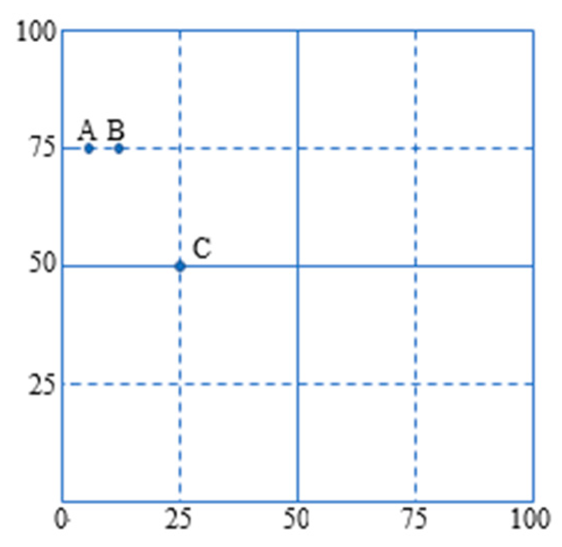
For instance, in Figure 1, the WSN has AREA = [0, 99) × [0, 99) and three sensors are labeled at A, B, and C located at (5, 75), (12, 75), and (25, 50), respectively. The RADIUS r(x, y) and COST(r(x, y)) for each sensor in the WSN in Figure 1 are provided in Table 1. From Table 1, the price needed for the sensor located at A to have RADIUS 10 is 4 units of cost., i.e., r(5, 75) = 10 and COST(r(5, 75)) = 4.

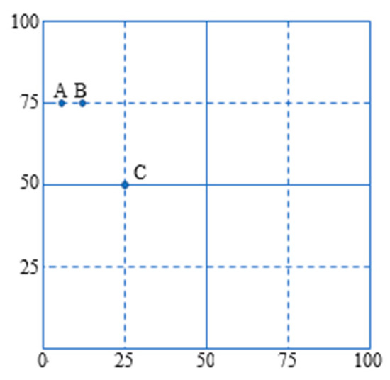
Figure 1. Example WSN.

Table 1. Information of the WSN in Figure 1.

i	(x, y)	Radius Level	r(x, y)	COST(r(x, y))
A	(5, 75)	1	1	1
		2	3	2
		3	5	3
		4	10	4
B	(12, 75)	1	2	1
		2	5	2
		3	8	3
C	(25, 50)	1	1	1
		2	2	2
		3	3	3
		4	4	4
		5	5	5

3.2. Effective Covered Grids and COST

Let |●| be the number of elements in ● and the sensing radius of the sensor located at (x, y) be r(x, y). In WSN(S, AREA, RADIUS, COST), the effectively covered grids ECG of the sensor in S located at (x, y) ϵ AREA is the set of grids inside the circle under radius r(x, y), i.e.,

ECG(r(x, y)) = { p | grid p is inside in CIRCLE(r(x, y)∩AREA },

(1)

where CIRCLE(r(x, y)) is the circle with center (x, y) and radius and r(x, y).

For example, in Figure 1, assume the sensor A located at (5, 75) is with r(A) = r(5, 75) = 10, and 255 grids are inside the circle under radius 10, i.e., the number of grids in { p | grid p is inside in (the circle with center and radius (5, 75) and r(5, 75)) } is 255. However, the area we are interested in is only in AREA = [0, 99) × [0, 99). Hence, these grids that are out of these range should be removed, i.e., (−1, 75), (−2, 75), (−3, 75), (−4, 75), (−5, 75), …., and 50 grids are removed because of this and only |ECG(r(5, 75) = 10)| = 255 grids are left.

The total ECG of a whole WSN is calculated based on Equation (1) after removing these grids outside AREA or in the intersection ranges of sensors as follows:

$${\displaystyle \underset{}{\cup }\mathrm{ECG}(r(x,y))} \mathrm{for} \mathrm{all} \mathrm{sensors} \mathrm{located} \mathrm{in} (x, y) \mathrm{with} \mathrm{radius} r(x, y)$$

(2)

The total grids coved by all sensors is:

$$|{\displaystyle \underset{}{\cup }\mathrm{ECG}(r(x,y)})|.$$

(3)

For example, |ECG(r(A) = 10)| = 255 as shown before, |ECG(r(B) = 8)| = 193, and |ECG(r(C) = 5)| = 69. There are 124 grids in ECG(r(A) = 10) ∩ ECG(r(B) = 8) and ECG(r(A) = 10) ∩ ECG(r(C) = 5) = ECG(r(B) = 8) ∩ ECG(r(C) = 5) = ∅, where sensors A, B, and C are located at (5, 75), (12, 75), and (25, 50), respectively. We have:

|ECG(r(A) = 10) ∩ ECG(r(B) = 8) ∩ ECG(r(C) = 5)|
   = 255 + 193 + 69 − 124 = 393.

(4)

Moreover, from COST in WSN(S, AREA, RADIUS, COST), if the cost of the sensor located in (x, y) with radius r(x, y) is COST(r(x, y)), the total cost to have the above deploy plan for all sensors in S is:

$${\displaystyle \sum _{(x,y)}\mathrm{COS}\mathrm{T}(r(x,y))}.$$

(5)

For the same example in Figure 1, based on Table 1, the cost to have r(A) = 10, (B) = 8, and r(C) = 5 is COST(r(A) = 10) = 4, COST(r(B) = 8) =3, and COST(r(C) = 5) =5. The total cost to achieve this is:

COST(r(A) = 10) + COST(r(B) = 8) + COST(r(C) = 5) = 12.

(6)

3.3. Proposed Mathematical Model

It is assumed that WSN(S, AREA, RADIUS, COST) are the WSN we considered, where the location, the levels of radius, and the prices of each radius level are all provided in S, RADIUS, and COST for each sensor, respectively. The proposed budget-limited WSN sensing coverage problem needs to determine the radius level for each sensor to have the maximal effective covered grids of the whole WSN under a limited budget to improve the WSN service quality.

A mathematical model for the problem is presented below:

$$\mathrm{Max}{\displaystyle \underset{(x,y)}{\cup }\mathrm{ECP}(r(x,y)})|$$

(7)

$$\mathrm{s}.\mathrm{t}. {\displaystyle \sum _{(x,y)}\mathrm{COS}\mathrm{T}(r(x,y))} \le \mathrm{COS}{\mathrm{T}}_{\mathrm{UB}}.$$

(8)

The objective function in Equation (7) maximizes the number of grids covered by sensors. The only constraint of Equation (8) is the budget-limited total cost of the sensors. Note that, if without Equation (8), each sensor can be set to its maximum radius level, i.e., it is impractical.

The proposed budget0-limited WSN sensing coverage problem is one of the variants of the knapsack problem. Hence, the proposed problem is also an NP-Hard problem, and it is impossible to be solved in polynomial time [22,23]. It is always necessary to have an efficient algorithm to solve the important and practical sensor problem. This study thus proposes a new algorithm based on SSO to overcome the NP-Hard obstacles to improve the SSO to enhance the obtained WSN service quality.

4. Proposed Novel Bi-Tuning SSO

The proposed bi-tuning SSO is based on SSO, and it inheres all characteristics from SSO, i.e., the population-based, the fixed-length solutions, evolution from generation to generation as the other algorithms in the evolution computing, a leader as other algorithms in the swarm intelligence, and the all-variable update such that each variable is updated based on the stepwise function update mechanism shown in Equation (9). The details, pseudo-code, explanation, and example of the proposed bi-tuning SSO are presented in this section. Moreover, the proposed method is verified/validated by the numerical experiments and the results obtained by the proposed bi-tuning SSO are compared with the state-of-art algorithms PSO, GA, and SSO in Section 6.

Solution Structure

As with most machine learning algorithms, the first step is to define the solution structure [1,2,3,4,5,6,7,8,9,37,38,39,40,41,42,43]. A solution in the proposed bi-tuning SSO for the proposed problem is defined as a vector, where the number of coordinates in each vector is the number of sensors, and the value, say k, of the ith coordinate of each vector is the radius level k of the ith sensor utilized in the WNS. For example, in Figure 1, let X₅ = (4, 3, 4) be the 5th solution in the current generation and the radius levels of sensors A, B, and C are 4, 3, and 5, i.e., r(5, 75) = 10, r(12, 75) = 8, and r(25, 50) = 5 in X₅, respectively.

5. Results

Proposed by Yeh in 2009 [31], the simplified swarm optimization (SSO) is said to be the simplest of all machine learning methods [13,14,21,22]. The SSO was initially called the discrete PSO (DPSO) to tackle the shortcomings of the PSO in discrete problems and is appealing due to its smooth and straightforward implementation, a fast convergence rate, and fewer parameters to tune, which has been shown by numerous related works of SSO, such as optimization of the vehicle routing in a supply chain [47], solving of reliability redundancy allocation problems [48,49], optimization of related problems in wireless sensor networks [42,50], resolving of redundancy allocation problems considering uncertainty [39,51], optimization of the capacitated facility location problems [52], improvement of the update mechanism of SSO [53], recognition of lesions in medical images [54], resolving of service in a traffic network [55], and optimization of numerous types of network research [56,57,58,59,60,61,62,63].

As a population-based stochastic optimization technique, the SSO belongs to the category of swarm intelligence methods with leaders to follow. The SSO is also an evolutionary computational method used to update the solution from generation to generation.

Moreover, SSO is a very influential tool in data mining for certain datasets [13,14,21] and is therefore implemented to solve the proposed budget-limited WSN sensing coverage problem.

5.1. Parameters

Each AI algorithm has its parameters in its update mechanism and/or the selection procedure, e.g., crossover rate c_x and mutation rate c_m in GA, c₁ and c₂ in PSO, and C_g, C_p, and C_w in the SSO, etc.

It is assumed that X_i, P_i, and P_gBest are the ith solution, the best ith solution in its evolutionary history, and the best solution among all solutions, respectively. Let x_i,j, p_i,j, and p_gBest,j be the jth variable of X_i, P_i, and P_gBest, respectively. SSO is the adapted all-variable update, i.e., all variables need to be updated, such that x_i,j is obtained from either p_gBest,j, p_i,j, x_i,j, and a random generated feasible value x with probabilities c_g, c_p, c_w, and c_r, respectively.

Because c_g + c_p + c_w + c_r = 1, there are three parameters to tune in SSO: C_g = c_g, C_p = C_g + c_p, and C_w = C_p + c_w. Additionally, in the proposed algorithm, c_g = 0.5, c_p = 0.95, and c_w = 0.95.

5.2. Update Mechanism

Hence, the update procedure of each variable can be presented as a stepwise-function:

$$x_{i,j}=\{\begin{array}{l}{p}_{gBest,j}\hfill \\ p_{i,j}\hfill \\ x_{i,j}\hfill \\ x\hfill \end{array}\begin{array}{l}{\mathrm{if} \mathsf{\rho }}_{[0,1]}\in [0,C_g) \hfill \\ {\mathrm{if} \mathsf{\rho }}_{[0,1]}\in [C_g,C_p)\hfill \\ {\mathrm{if} \mathsf{\rho }}_{[0,1]}\in [C_p,C_w)\hfill \\ {\mathrm{if} \mathsf{\rho }}_{[0,1]}\in [C_w, 1]\hfill \end{array}$$

(9)

where ρ_[0,1] is a random number generated within [0,1] consistently.

From Equation (9), the update in SSO is simple to code, runs efficiently, and flexible amd made-to-fit [20,23,24,25,26,27,28,46]. Each AI algorithm has its own update mechanism, e.g., crossover and mutation in GA, vectorized update mechanism in PSO, etc. The stepwise update function is a unique update mechanism of SSO [23,24,37,38,39,40,41,42]. All SSO variants are based on their made-to-fit stepwise function to update solutions.

The stepwise-function update mechanism shown in Equation (9) is powerful, straightforward, and efficient with proven success, as evidenced through successful applications, e.g., the redundancy allocation problem [37,38], disassembly sequencing problem [39,40], artificial neural network [41], energy problems [42], etc. Moreover, the stepwise-function update mechanism allows for greater ease of customization to made-to-fit by replacing any item of its stepwise function with other algorithms [38,41], even hybrid algorithms [43] applied in sequence or parallel [41], to address different problems as opposed to tedious customization of other algorithms [23,24,37,38,39,40,41,42,43].

5.3. Pseudocode, Flowchart, and Example

The SSO is very easy to code using any computer language and its pseudocode is provided below [17,18,35,36,37,38,39]:

STEP S0. 

Generate P_i = X_i randomly, calculate F(P_i) = F(X_i), find gBest, and let t = 1 and k = 1 for i = 1, 2, …, N_sol.

STEP S1. 

Update X_k based on Equation (9).

STEP S2. 

If F(X_k) > F(P_k), let P_k = X_k. Otherwise, go to STEP S5.

STEP S3. 

If F(P_k) > F(P_gBest), let gBest = k.

STEP S4. 

If k < N_sol, let k = k + 1 and go to STEP S1.

STEP S5. 

If t < N_gen, let t = t + 1, k = 1, and go to STEP S1. Otherwise, halt.

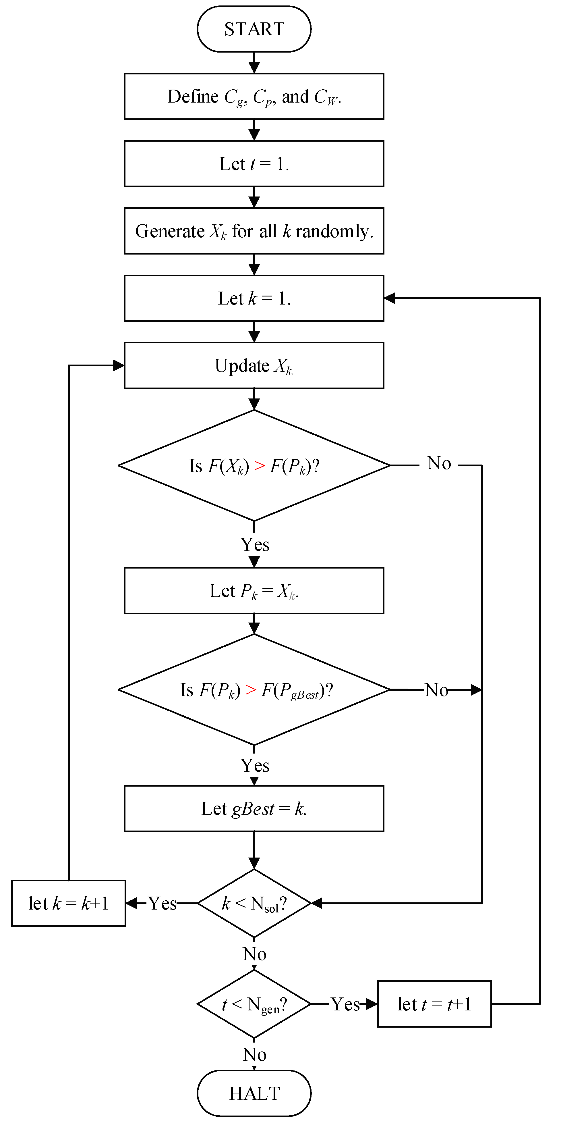
The flowchart of the above pseudocode is given in Figure 2:

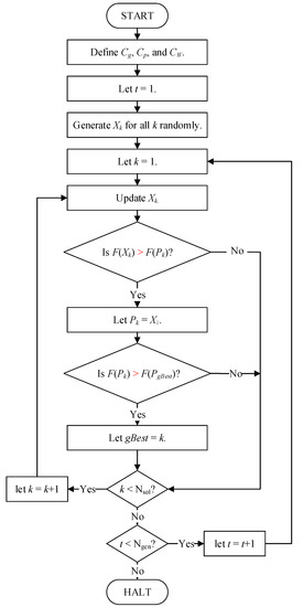
Figure 2. The flowchart of SSO.

STEP S0 initializes all solutions randomly because the SSO is a population-based algorithm. STEP S1 implements the SSO stepwise function shown in Equation (9) to update the solution. STEPs S2 and S3 test whether P_k is replaced with X_k and P_gBest is replaced with P_k, respectively. STEP S5 is the stopping criteria, which is the number of generations. Note that the stopping criteria are changed to the runtime in this study and the details are discussed in Section 4.

For example, let C_g = 0.4, C_p = 0.7, C_w = 0.9, and ρ = (ρ₁, ρ₂, ρ₃, ρ₄, ρ₅) = (0.53, 0.78, 0.16, 0.97, 0.32). Assume that we have the solution in the second generation, i.e., X₁₅ = (4, 3, 2, 1, 4), P₁₅ = (1, 4, 2, 3, 2), and P_gBest = (1, 4, 2, 3, 2), which are the 15 solutions in the second generation of the evolutionary, the best 15 solutions before the second generation, and the best solution before the second generation, respectively. Now, we are going to update X₁₅ to obtain the new X₁₅ of the third generation, which is presented in Table 2, based on the stepwise function of the SSO update mechanism provided in Equation (9).

Table 2. An example of the SSO update process.

Variable	1	2	3	4	5
X15	4	3	2	1	4
X	1	4	3	3	2
ρ	0.53	0.78	0.16	0.97	0.32
New X15	1	3	3	4 #	2

“^#” indicates that the value is generated randomly in a feasible region.

From the above pseudocode, flowchart, and example, we can find that the update mechanism of the SSO is simple, convenient, and efficient.

5.4. Fitness Function and Penalty Fitness Function

The fitness function F(X) guides solution X towards optimization, which, in turn, will attain goals in artificial intelligence, such as the SSO, GA, and PSO. All suitable fitness functions vary, depending on the optimization problem defined by the corresponding application. In this study, Equation (7) is adopted here to represent the fitness function, which is to be maximized in the proposed problem. For example, without considering the budget limit, F(X₅) = 393, as discussed in Equation (4) for X₅ = (4, 3, 4).

The penalty fitness function F_P(X) helps deal with these problems without too many constraints and it is not easy to generate feasible solutions that satisfy the constraints, e.g., Equation (5). Penalty functions can force these infeasible solutions near the feasible boundary back to the feasible region by adding or subtracting larger positive values to the fitness for the maximum or minimum problems, respectively.

If the larger positive value is not large enough, the final solution may be not feasible. Hence, a novel self-adaptive penalty function based on the budget and the deploy plan is provided below:

$$F_{\mathrm{p}}(X)=\{\begin{array}{ll}F(X)-PENALTY\hfill & \mathrm{if} {\displaystyle \sum _{(x,y)}\mathrm{COS}\mathrm{T}(r(x,y))}>{\mathrm{COS}\mathrm{T}}_{\mathrm{UB}}\hfill \\ F(X)\hfill & \mathrm{otherwise}\hfill \end{array}$$

(10)

where:

$$\mathit{PENALTY}(X) = {\left[r_{\mathrm{UB}}{\displaystyle \sum _{(x,y)}\mathrm{COS}\mathrm{T}(r(x,y))}\right]}^2$$

(11)

For example, let COST_UB = 10 in Figure 1. The total cost for the fifth solution X₅ = (4, 3, 4) is COST(X₅) = COST(4, 3, 4) = 12 from Equation (6). Because COST(X₅) =12 > 10, we have:

PENALTY(X₅) = (10 × 12)² = 14,400,

The penalty fitness function of X₅ is:

F_p(X₅) = F(X₅) − PENALTY(X₅) = 393 − 14,400 = −14,007,

Here, the penalty fitness function is that the fitness function subtracts the penalty if the cost is over the COST_UB.

5.5. The Bi-Tuning Method

All machine learning algorithms have their parameters in each update procedure and/or the selection procedure. Thus, there is a need to tune parameters for better results. In the SSO, there are already two main concerns regarding the improvement of the solution quality by either focusing on the parameter-tuning to tune parameters or paying attention to the item-tuning to remove an item from Equation (9), e.g., Equations (12) and (13) remove the second and the third items from Equation (9). However, none of them can deal with the above two processes, i.e., the parameter-tuning and the item-tuning, at the same time:

$$x_{i,j}=\{\begin{array}{l}{p}_{gBest,j}\hfill \\ x_{i,j}\hfill \\ x\hfill \end{array}\begin{array}{l}{\mathrm{if} \mathsf{\rho }}_{[0,1]}\in [0,C_g) \hfill \\ {\mathrm{if} \mathsf{\rho }}_{[0,1]}\in [C_g=C_p,C_w)\hfill \\ {\mathrm{if} \mathsf{\rho }}_{[0,1]}\in [C_w, 1]\hfill \end{array}$$

(12)

$$x_{i,j}=\{\begin{array}{l}{p}_{gBest,j}\hfill \\ p_{i,j}\hfill \\ x\hfill \end{array}\begin{array}{l}{\mathrm{if} \mathsf{\rho }}_{[0,1]}\in [0,C_g) \hfill \\ {\mathrm{if} \mathsf{\rho }}_{[0,1]}\in [C_g,C_p)\hfill \\ {\mathrm{if} \mathsf{\rho }}_{[0,1]}\in [C_p=C_w,1]\hfill \end{array}$$

(13)

Hence, a new bi-tuning method is provided to achieve the above goal to determine the best parameters C_p, C_p, and C_w together with the best solution to answer whether any item in Equation (9) should be removed to obtain a better result.

Seven different settings are adapted and named as SSO1–SSO7 as shown in Table 3.

Table 3. Seven parameter settings.

SSOi	Cg	Cp	Cw	Remark
SSO1	0.4	0.7	0.9
SSO2	0.4	0.4	0.7	No Item 2, high cr
SSO3	0.4	0.4	0.9	No Item 2
SSO4	0.4	0.7	0.7	No Item 3, high cr
SSO5	0.7	0.7	0.9	No Item 2, high cg
SSO6	0.4	0.9	0.9	No Item 3
SSO7	0.7	0.9	0.9	No Item 3, high cg

If C_g = C_p in SSO2, SSO3, and SSO5 or C_p = C_w in SSO4, SSO6, and SSO7, the items 2 or 3 are redundant, i.e., P_i is never used as in Equation (12) and x_i,j must be replaced with a value as shown in Equation (13), respectively, from Table 3.

Additionally, SSO2 and SSO4 are used to test whether having a larger value of c_r = 1 − C_w is useful in improving the efficiency and solution quality. Similarly, SSO5 and SSO7 are applied to determine whether having a larger value of c_g = C_g improves the efficiency and solution quality.

5.6. Pseudocode of Bi-Tuning SSO

The bi-tuning SSO is a new SSO and can be used to tune both the parameters, i.e., C_g, C_p, and C_w, and update the mechanism in the traditional SSO efficiently and easily. The pseudocode of the proposed bi-tuning SSO is designated for the budget-limited WSN sensing coverage problem by the following procedures:

STEP 0. 

Let i = 1.

STEP 1. 

The parameters of SSOi are listed in Table 3 and let the best solution be G_i.

STEP 2. 

If i < 8, go to STEP 1.

STEP 3. 

The best one among G₁, G₂, …, and G₇, is the one we need.

It is always a very critical task to determine the time complexity of any algorithms and the time complexity is always based on the worst time complexity, i.e., the O-notation. Additionally, the time complexity of the fitness calculation depends on the problems and was ignored in some studies. Hence, due to the simplicity of the SSO, the computational complexity of the proposed bi-tuning SSO is determined mainly by the update mechanism.

The proposed bi-tuning SSO implementing the all-variable update mechanism needs to be run N_var times for each solution in each generation. Hence, the time complexity of the proposed bi-tuning SSO is O(7 × N_gen × N_sol × N_var). Furthermore, the practical performance of the proposed bi-tuning SSO was tested for nine problems, as described in Section 5.

6. Numerical Experiments

To demonstrate the performance of the proposed bi-tuning SSO, three numerical experiments with three different values of N_var = 20, 100, and 300 were implemented based on the bi-tuning method mentioned in Section 5.3. Similar published literature to this work could not be found so the experimental results of the bi-tuning SSO could not be compared with any other published contribution. However, the experimental results of the bi-tuning SSO were compared with the state-of-the-art algorithms PSO, GA, and SSO, which are listed as SSO1 in Table 3.

6.1. Parameters and Experimental Environment Settings

The performance of each AI algorithm is always affected by the parameter setting and experimental environment setting. The parameter settings for both GA and PSO are listed below:

• The crossover rate c_x = 0.7, the mutation rate c_m = 0.3, and elite selection.
• c₁ = c₂ =2.0, w = 0.95, the lower and upper bounds of velocities V_LB = −2 and V_UB = 2, the lower and upper bounds of positions X_LB = 1 and X_UB = the maximum radius.

Nine algorithms were tested, i.e., the bi-tuning SSO included seven SSO variants based on Table 3, GA, and PSO. To perform a fair performance evaluation of all algorithms, each algorithm was run 30 times, i.e., N_run = 30, with N_sol = 100, and the stopping criteria were based on the run time, which was defined as Nvar/10 s.

All algorithms were tested on three datasets, where the coordinate of X has a uniform distribution: 0 ~ (square of the number of vertices/32767)/(the number of vertices) and the coordinate of Y has a uniform distribution: 0 ~ (square of the number of vertices/32767)-the coordinate of X*(the number of vertices). Without loss of generality, each dataset has 1000 data of which the ith data in the dataset is a 2-tuple vector (x, y) representing the location of the ith sensor and it was generated randomly within [0,99] × [0,99] based on the grid concept. To verify the capacity of the proposed bi-tuning SSO, each dataset was separated into sub datasets based on the number of sensors N_var = 20, 100, and 300 by choosing the first N_var data to denote small-sized, middle-sized, and larger-sized problems.

All nine algorithms including the proposed bi-tuning SSO were coded in DEV C++ on a 64-bit Windows 10 PC, implemented on an Intel Core i7-6650U CPU @ 2.20 GHz notebook with 16 GB of memory.

6.2. Analysis of Results

The descriptive statistics including the maximum (denoted by MAX), i.e., the best solution, minimum (denoted by MIN), average (denoted by AVG), and standard deviation (denoted by STD) of the run time (denoted by T, in seconds), fitness function value (denoted by F), number of generations to obtain the optimal solution (denoted by Best), how many generations were run during the provided time (denoted by Ngen), and total cost (denoted by Cost) were employed for the nine algorithms including GA, PSO, and the proposed bi-tuning SSO including seven SSO variates (denoted by SSO1 to SSO7) and the best solutions compared among the nine algorithms are shown in bold. Hence, the following Table 4, Table 5 and Table 6 indicate the experimental results obtained by all algorithms for the first dataset to the third dataset of the small-sized problem, Table 7, Table 8 and Table 9 indicate the experimental results obtained by all algorithms for the first dataset to the third dataset of the middle-sized problem, and Table 10, Table 11 and Table 12 indicate the experimental results obtained by all algorithms for the first dataset to the third dataset of the larger-sized problem.

Table 4. The experimental results obtained by all algorithms for the first dataset of the small-sized problem.

		GA	PSO	SSO1	SSO2	SSO3	SSO4	SSO5	SSO6	SSO7
MAX	T	30.016	30.03	30.019	30.019	30.017	30.018	30.017	30.017	30.013
	F	9978	9865	9983	9983	9983	9983	9983	9983	9979
	Best	478	2	2380	2208	2552	2045	2749	2497	2494
	Ngen	3018	1641	2742	2791	2767	2788	2782	2771	2790
	Cost	1722	2197	1827	1790	1826	1831	1841	1785	1845
MIN	T	30	30	30	30	30	30	30.001	30	30
	F	9978	9731	9978	9978	9978	9978	9978	9977	9978
	Best	1	0	574	335	832	231	607	294	521
	Ngen	1535	873	1475	1501	1490	1489	1495	1481	1495
	Cost	1635	1648	1674	1638	1622	1644	1661	1650	1641
AVG	T	30.00553	30.01207	30.00567	30.00627	30.00673	30.0063	30.00667	30.00613	30.00593
	F	9978	9792.66667	9978.83333	9979.8	9978.7	9979.83333	9978.93333	9978.33333	9978.03333
	Best	35	1.066667	1241.667	1069.033	1289.8	795.6	1331	1146.433	1158.2
	Ngen	2599.067	1426.033	2360.933	2398.1	2373.067	2378.5	2395.367	2411.667	2434.2
	Cost	1691.1	2056.367	1727.833	1715.567	1728.667	1722.833	1723.467	1728.5	1716.9
STD	T	0.004599	0.006987	0.004482	0.004017	0.005044	0.003975	0.00396	0.004175	0.003629
	F	0	32.91822	1.743626	2.171921	1.643168	2.450663	1.779836	1.295439	0.182574
	Best	108.4305	0.52083	431.9754	498.3848	309.4652	516.4621	560.7543	405.5847	323.8453
	Ngen	578.9797	311.1447	540.8861	548.114	543.0889	547.7753	549.496	522.6493	527.1815
	Cost	32.00361	114.8488	38.0889	36.7214	44.82251	47.97132	42.68468	34.85413	51.97304

Table 5. The experimental results obtained by all algorithms for the second dataset of the small-sized problem.

		GA	PSO	SSO1	SSO2	SSO3	SSO4	SSO5	SSO6	SSO7
MAX	T	30.018	30.033	30.02	30.015	30.02	30.018	30.019	30.02	30.018
	F	9989	9884	9983	9983	9983	9983	9983	9983	9983
	Best	2145	2	2551	2700	1872	2438	1998	2347	1482
	Ngen	2959	1646	2767	2825	2774	2788	2777	2772	2796
	Cost	1693	2182	1827	1825	1823	1831	1823	1807	1811
MIN	T	30	30	30	30	30	30	30	30	30
	F	9978	9741	9978	9978	9977	9978	9978	9978	9978
	Best	1	1	341	366	210	229	667	248	496
	Ngen	1516	872	1482	1505	1490	1480	1492	1479	1493
	Cost	1663	1969	1603	1640	1614	1620	1646	1621	1665
AVG	T	30.00657	30.01023	30.0067	30.00597	30.00803	30.00703	30.00463	30.0082	30.00833
	F	9981.4	9788.6	9978.53333	9978.83333	9978.3	9979.3	9978.73333	9978.4	9978.33333
	Best	185.8333	1.133333	1204.767	1029.1	1141.767	786.1333	1247.133	1073.7	1105.133
	Ngen	2274.467	1293.033	2225.5	2245.933	2199.867	2200.767	2198.8	2179.367	2205.5
	Cost	1682.6	2085.333	1727.967	1735.867	1718.533	1733.9	1729.467	1723.167	1739.2
STD	T	0.005022	0.008597	0.005503	0.004287	0.005295	0.004642	0.00476	0.005886	0.005542
	F	4.553135	31.44848	1.332183	1.821014	1.055364	1.985291	1.740657	1.302517	1.093345
	Best	495.5494	0.345746	487.2496	624.9864	344.4217	525.9668	289.8154	365.2003	202.0889
	Ngen	679.1606	372.5816	614.4892	621.035	625.3054	632.8352	620.3057	616.5297	626.747
	Cost	11.99598	55.71995	50.17932	44.33395	54.67505	51.75363	42.43269	48.42063	31.55881

Table 6. The experimental results obtained by all algorithms for the third dataset of the small-sized problem.

		GA	PSO	SSO1	SSO2	SSO3	SSO4	SSO5	SSO6	SSO7
MAX	T	30.018	30.032	30.02	30.019	30.019	30.019	30.018	30.018	30.017
	F	9978	9853	9983	9983	9982	9983	9983	9983	9983
	Best	276	2	1802	2401	2365	2184	2421	1490	2611
	Ngen	3021	1644	2771	2801	2778	2772	2818	2749	2775
	Cost	1752	2200	1826	1791	1803	1802	1820	1807	1812
MIN	T	30	30	30.001	30	30	30	30.001	30	30
	F	9978	9730	9978	9978	9977	9978	9978	9978	9978
	Best	1	1	387	363	511	243	593	508	261
	Ngen	1566	871	1476	1505	1488	1488	1488	1480	1491
	Cost	1649	1964	1639	1606	1616	1651	1619	1592	1642
AVG	T	30.00683	30.01213	30.00733	30.00757	30.0082	30.0067	30.00727	30.00813	30.00743
	F	9978	9795.6	9978.5	9979.23333	9978.2	9979.36667	9978.5	9978.16667	9978.23333
	Best	23.06667	1.1	1082.867	981.5	1301.467	801	1220.067	1118.167	1149.433
	Ngen	2262.133	1265.833	2094.033	2104.067	2065	2095.933	2139.733	2126.267	2150.867
	Cost	1694.3	2084.033	1719.3	1715.4	1714.2	1734.9	1726.3	1729.233	1731.8
STD	T	0.005079	0.009164	0.005504	0.005799	0.005536	0.005447	0.004668	0.005619	0.00424
	F	0	26.92851	1.525643	1.95965	0.846901	2.07586	1.525643	0.912871	0.971431
	Best	68.5228	0.305129	313.4875	451.0136	400.4922	523.9492	432.6585	195.9879	403.8005
	Ngen	619.5315	372.9234	617.1579	622.4222	618.3723	613.6447	608.3816	608.3502	617.2854
	Cost	43.49645	56.33611	41.50958	43.59263	42.46573	40.95106	49.34897	49.96598	43.29163

Table 7. The experimental results obtained by all algorithms for the first dataset of the middle-sized problem.

		GA	PSO	SSO1	SSO2	SSO3	SSO4	SSO5	SSO6	SSO7
MAX	T	30.01	30.017	30.009	30.01	30.011	30.011	30.01	30.01	30.01
	F	9978	9846	9983	9983	9983	9983	9983	9983	9983
	Best	673	2	2641	2149	2527	2635	1770	2672	2624
	Ngen	3084	1642	2767	2818	2816	2778	2811	2782	2792
	Cost	1801	2165	1819	1810	1831	1796	1849	1828	1836
MIN	T	30	30.001	30	30.001	30	30	30	30	30
	F	9978	9739	9978	9978	9978	9978	9978	9978	9978
	Best	1	0	693	412	859	246	561	761	704
	Ngen	2651	1567	2644	2688	2665	2625	2662	2633	2661
	Cost	1684	1673	1631	1652	1664	1640	1642	1628	1636
AVG	T	30.00507	30.0088	30.00473	30.00627	30.0053	30.00513	30.00437	30.00493	30.00503
	F	9978	9788.6	9978.533	9979.767	9978.7	9979.5	9978.6	9978.867	9978.867
	Best	48.6	1	1232.933	1044.867	1370.533	861.9	1129.6	1322	1303.567
	Ngen	2873.667	1604.2	2694.5	2743.833	2714.6	2713.967	2729.967	2695.067	2726.133
	Cost	1725.8	2045.167	1726.6	1724.633	1741.9	1722.8	1727.667	1725.467	1729.933
STD	T	0.002935	0.005307	0.00269	0.003226	0.003271	0.003309	0.002953	0.003205	0.003211
	F	0	24.85905	1.525266	2.387949	1.664021	2.23992	1.588754	1.696514	1.696514
	Best	163.2047	0.371391	346.3405	484.3381	402.4024	612.3711	235.5152	447.2216	499.3975
	Ngen	145.576	24.71688	37.99887	39.11793	38.88054	37.50355	43.45309	42.34011	37.0086
	Cost	52.06521	89.08117	44.78654	46.75209	38.79686	46.54282	43.94615	41.61128	56.03689

Table 8. The experimental results obtained by all algorithms for the second dataset of the middle-sized problem.

		GA	PSO	SSO1	SSO2	SSO3	SSO4	SSO5	SSO6	SSO7
MAX	T	30.016	30.03	30.019	30.017	30.02	30.017	30.019	30.019	30.02
	F	9983	9868	9983	9983	9983	9983	9983	9983	9983
	Best	1856	2	1766	2479	2231	2560	2573	2472	1502
	Ngen	2909	1652	2784	2814	2786	2797	2826	2780	2801
	Cost	1806	2189	1835	1815	1852	1819	1812	1849	1819
MIN	T	30	30	30	30	30	30	30	30	30
	F	9978	9745	9978	9978	9976	9978	9977	9978	9978
	Best	1	0	667	349	635	345	616	881	459
	Ngen	1433	869	1482	1502	1485	1487	1493	1477	1488
	Cost	1671	1653	1637	1648	1602	1625	1673	1630	1653
AVG	T	30.00633	30.01093	30.00553	30.00713	30.00693	30.00717	30.00723	30.00753	30.0065
	F	9978.167	9793.167	9978.333	9978.833	9978.467	9979.9	9978.8	9978.933	9978.467
	Best	105	1.133333	1146.4	946.8333	1241.033	807.1333	1183.8	1357.7	1070.633
	Ngen	2275.867	1312.067	2201.533	2238.867	2215.833	2218.733	2237.3	2212.9	2233.933
	Cost	1740.2	2034.633	1734.6	1723.2	1720.4	1716.267	1731.067	1743.767	1729.733
STD	T	0.004498	0.007575	0.004337	0.004981	0.004623	0.004706	0.005104	0.005507	0.004305
	F	0.912871	31.09394	1.268541	1.662639	1.696514	2.264417	1.845778	1.700575	1.431983
	Best	357.3568	0.571346	234.341	461.4511	342.0513	585.8245	419.4534	436.2568	258.3106
	Ngen	649.3819	364.3246	591.1066	607.9616	598.1902	603.5461	612.5769	605.9686	606.409
	Cost	54.56056	147.6306	43.0754	47.85495	52.24914	53.50858	37.76235	50.28106	42.17528

Table 9. The experimental results obtained by all algorithms for the third dataset of the middle-sized problem.

		GA	PSO	SSO1	SSO2	SSO3	SSO4	SSO5	SSO6	SSO7
MAX	T	30.016	30.029	30.015	30.019	30.02	30.017	30.019	30.017	30.02
	F	9983	9840	9983	9983	9983	9983	9983	9983	9983
	Best	665	2	2719	1513	2458	2725	2657	2616	2622
	Ngen	2974	1634	2771	2802	2782	2774	2785	2760	2785
	Cost	1734	2172	1817	1823	1847	1836	1842	1776	1822
MIN	T	30	30	30	30	30	30	30	30	30
	F	9978	9753	9978	9978	9978	9978	9978	9977	9977
	Best	1	1	462	409	530	299	740	473	685
	Ngen	1488	872	1473	1501	1485	1483	1488	1480	1493
	Cost	1699	1818	1641	1630	1651	1625	1686	1648	1622
AVG	T	30.0057	30.01187	30.00653	30.00743	30.00647	30.00633	30.006	30.0056	30.0082
	F	9980.5	9789.333	9978.933	9978.867	9978.4	9980.633	9978.633	9979.1	9978.767
	Best	46.26667	1.133333	1249.467	919.8667	1317.2	998.0667	1232.767	1320.133	1241.3
	Ngen	2370.833	1357.267	2293.7	2337.167	2309.1	2309.567	2311.667	2289.633	2315.233
	Cost	1706.167	2066.033	1730.533	1717.533	1728.3	1732.167	1734.933	1721.967	1708.9
STD	T	0.004625	0.007651	0.003767	0.00436	0.00529	0.004373	0.005092	0.004753	0.005567
	F	2.542738	24.92933	1.779836	1.73669	1.302517	2.413801	1.401559	2.023142	1.794308
	Best	137.1495	0.345746	464.0115	292.5383	432.6933	723.7991	424.38	562.7488	399.9335
	Ngen	616.4583	347.2867	584.6227	595.5204	587.5019	588.599	584.5419	579.4924	585.9167
	Cost	8.021881	87.69126	48.1139	48.22843	41.46469	45.28232	44.29597	31.96926	53.11429

Table 10. The experimental results obtained by all algorithms for the first dataset of the larger-sized problem.

		GA	PSO	SSO1	SSO2	SSO3	SSO4	SSO5	SSO6	SSO7
MAX	T	30.008	30.016	30.011	30.01	30.01	30.01	30.011	30.011	30.011
	F	9981	9821	9983	9983	9983	9983	9983	9983	9983
	Best	2177	2	2375	2712	2159	2672	2457	2190	2327
	Ngen	3140	1648	2752	2820	2789	2771	2795	2761	2790
	Cost	1768	2196	1816	1815	1813	1795	1776	1884	1821
MIN	T	30	30	30	30	30	30	30	30	30
	F	9978	9735	9978	9978	9978	9978	9978	9978	9978
	Best	1	1	325	67	206	251	396	511	471
	Ngen	2722	1569	2632	2676	2659	2667	2668	2640	2673
	Cost	1622	1962	1629	1636	1647	1659	1623	1622	1650
AVG	T	30.00393	30.0088	30.00623	30.00503	30.005	30.00587	30.00533	30.00547	30.00433
	F	9978.3	9777	9979.067	9979.833	9978.433	9980.6	9978.667	9978.833	9978.567
	Best	94.83333	1.2	1303.767	1127.133	1265.567	985.7667	1213.833	1245.967	1179.167
	Ngen	2913.6	1604.933	2696.867	2751.233	2717.533	2724.3	2725.3	2700.033	2735
	Cost	1709.5	2104.5	1723.033	1716.333	1724	1726.533	1719.133	1741	1730.533
STD	T	0.002803	0.005242	0.003234	0.003057	0.003206	0.003441	0.003387	0.003421	0.003642
	F	0.915386	20.35716	2.03306	2.290661	1.356551	2.343001	1.604591	1.78274	1.50134
	Best	398.6142	0.406838	488.6539	623.4962	323.6076	628.7728	458.7228	354.8188	388.8087
	Ngen	128.3596	23.43286	34.89861	39.51402	32.91235	35.7319	32.52389	35.1553	34.02433
	Cost	49.21715	54.57848	42.06931	49.62225	37.42118	37.48446	38.59939	52.92936	50.27081

Table 11. The experimental results obtained by all algorithms for the second dataset of the larger-sized problem.

		GA	PSO	SSO1	SSO2	SSO3	SSO4	SSO5	SSO6	SSO7
MAX	T	30.017	30.029	30.02	30.018	30.017	30.015	30.019	30.02	30.016
	F	9983	9846	9983	9983	9983	9983	9983	9983	9983
	Best	394	2	2710	2713	2532	2697	2631	2442	2073
	Ngen	2864	1657	2767	2817	2769	2783	2796	2768	2818
	Cost	1801	2187	1799	1816	1813	1819	1803	1813	1819
MIN	T	30	30.001	30	30	30	30	30	30	30
	F	9978	9741	9978	9978	9978	9978	9978	9978	9977
	Best	1	1	387	364	377	236	596	696	645
	Ngen	1531	872	1484	1502	1490	1484	1494	1475	1494
	Cost	1701	1935	1647	1609	1611	1629	1691	1584	1627
AVG	T	30.00697	30.0104	30.00737	30.0068	30.00703	30.0056	30.00683	30.00683	30.0049
	F	9978.333	9783.467	9978.9	9979.6	9978.7	9980.233	9978.367	9978.8	9978.567
	Best	32.66667	1.2	1308.167	1091.667	1366.567	826.9667	1152.1	1177.767	1197.967
	Ngen	2374.6	1367.267	2313.167	2349.767	2318.333	2317.533	2327.833	2302.867	2335
	Cost	1728.5	2081.4	1723.767	1722.233	1731.267	1733.9	1741.4	1720.267	1729.033
STD	T	0.004745	0.007458	0.005518	0.0062	0.004148	0.003847	0.004276	0.005004	0.004254
	F	1.268541	24.35334	1.688705	2.061135	1.512021	2.373464	1.159171	1.517712	1.612095
	Best	92.56213	0.406838	463.87	672.524	429.0404	666.143	351.8519	410.7493	302.1507
	Ngen	599.9939	354.6363	594.3977	605.5757	590.8207	596.3299	592.7199	590.2427	598.3591
	Cost	18.92225	57.324	41.77005	47.04707	44.165	41.1099	26.55976	50.98609	48.81102

Table 12. The experimental results obtained by all algorithms for the third dataset of the larger-sized problem.

		GA	PSO	SSO1	SSO2	SSO3	SSO4	SSO5	SSO6	SSO7
MAX	T	30.015	30.032	30.019	30.012	30.019	30.014	30.018	30.019	30.017
	F	9978	9845	9981	9983	9983	9983	9983	9983	9983
	Best	209	2	2041	2733	2158	2574	2596	2391	1907
	Ngen	2959	1640	2756	2817	2775	2783	2812	2772	2783
	Cost	1686	2191	1840	1818	1833	1841	1847	1792	1808
MIN	T	30	30	30	30	30	30	30.001	30	30
	F	9978	9745	9978	9978	9978	9978	9978	9978	9978
	Best	1	0	677	538	350	148	764	510	554
	Ngen	1548	873	1477	1502	1489	1491	1498	1477	1494
	Cost	1666	1828	1648	1636	1613	1634	1641	1620	1592
AVG	T	30.0052	30.00927	30.00637	30.00527	30.00647	30.00663	30.0062	30.00567	30.00687
	F	9978	9789.267	9978.3	9980.1	9978.267	9979.6	9978.433	9978.767	9978.4
	Best	19.23333	1.133333	1155.067	1212.367	1178.033	872.4667	1164.867	1213	1255
	Ngen	2657.467	1491.2	2468.967	2549.4	2519.267	2527.5	2531.967	2503.5	2530.467
	Cost	1683.067	2069.567	1736.867	1720.667	1725.4	1741.1	1739.233	1721.7	1716.3
STD	T	0.004318	0.007674	0.005	0.003723	0.004455	0.004165	0.004021	0.005435	0.00471
	F	0	27.33185	0.915386	2.354013	0.980265	2.23761	1.356551	1.654322	1.132589
	Best	56.19896	0.434172	312.2639	595.2987	366.6347	719.0704	364.0858	368.7952	273.7001
	Ngen	525.0898	280.644	479.5429	473.2856	466.1362	470.4982	468.2634	463.8382	467.6395
	Cost	4.15172	87.34619	44.09921	40.41111	49.08304	40.95948	47.64718	44.49963	53.89079

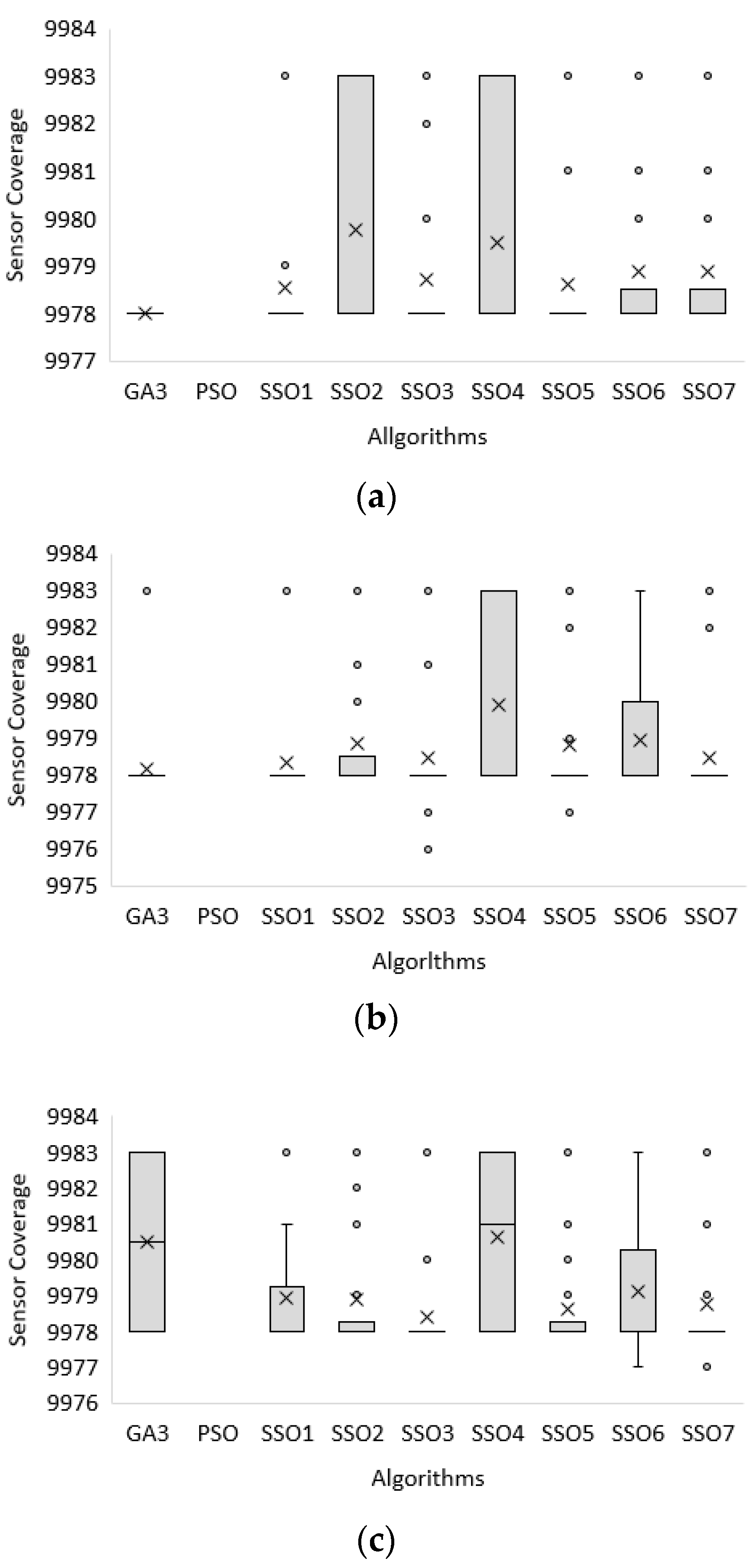
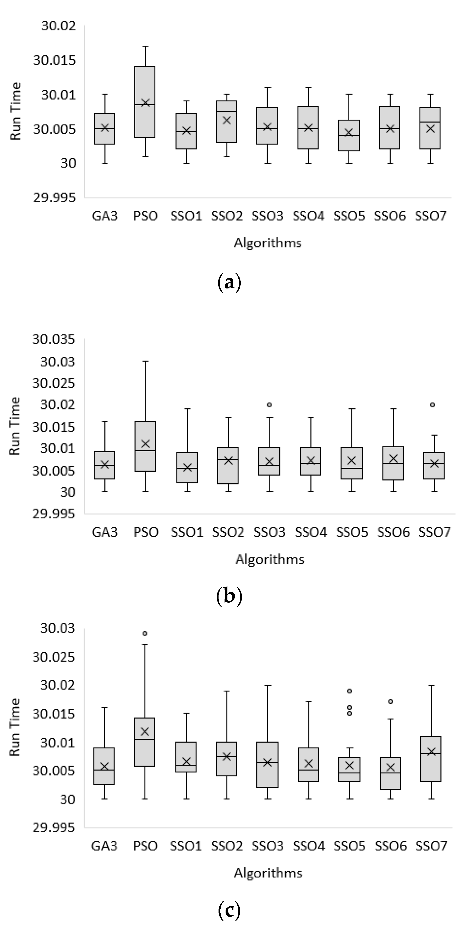
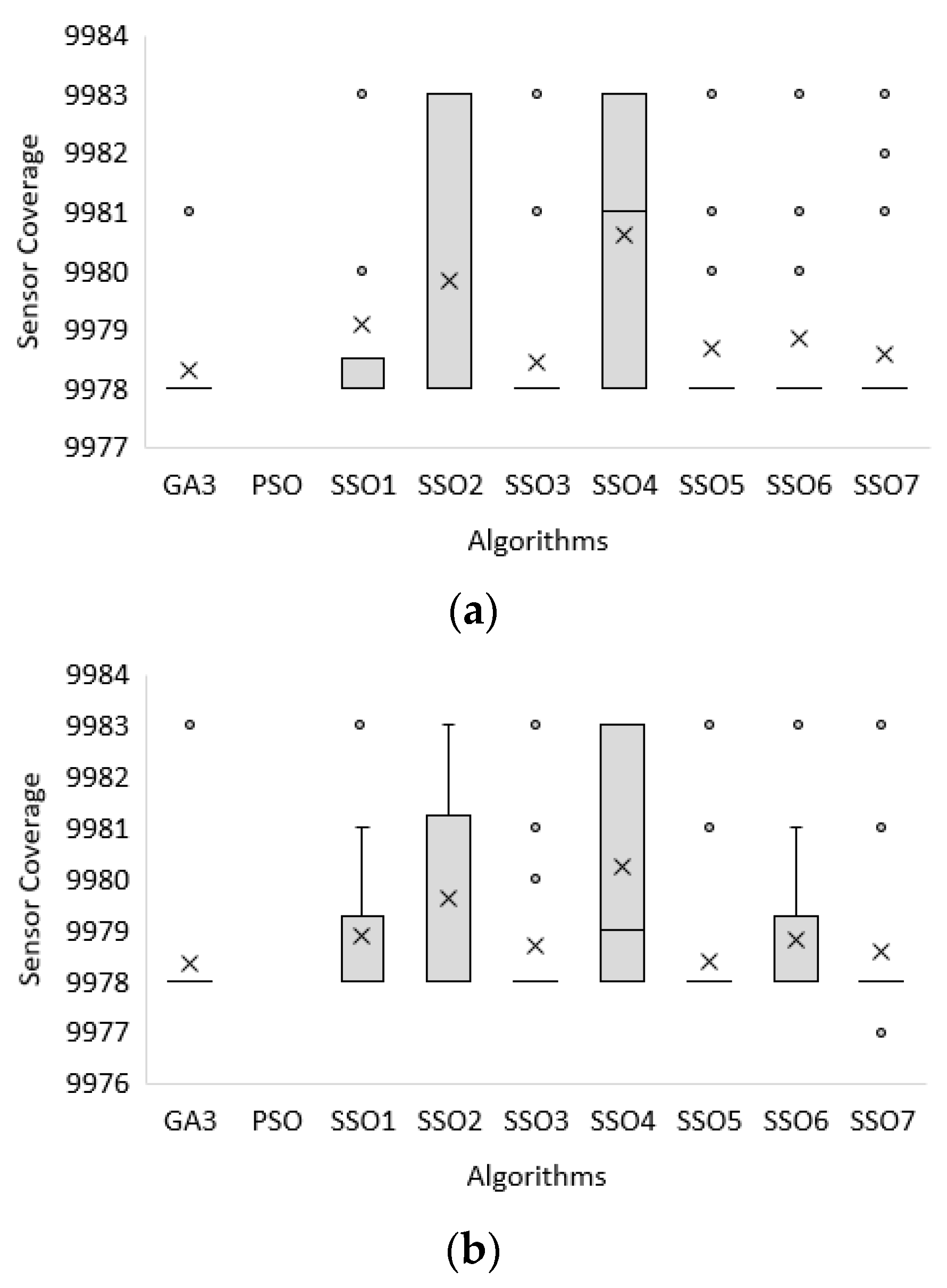
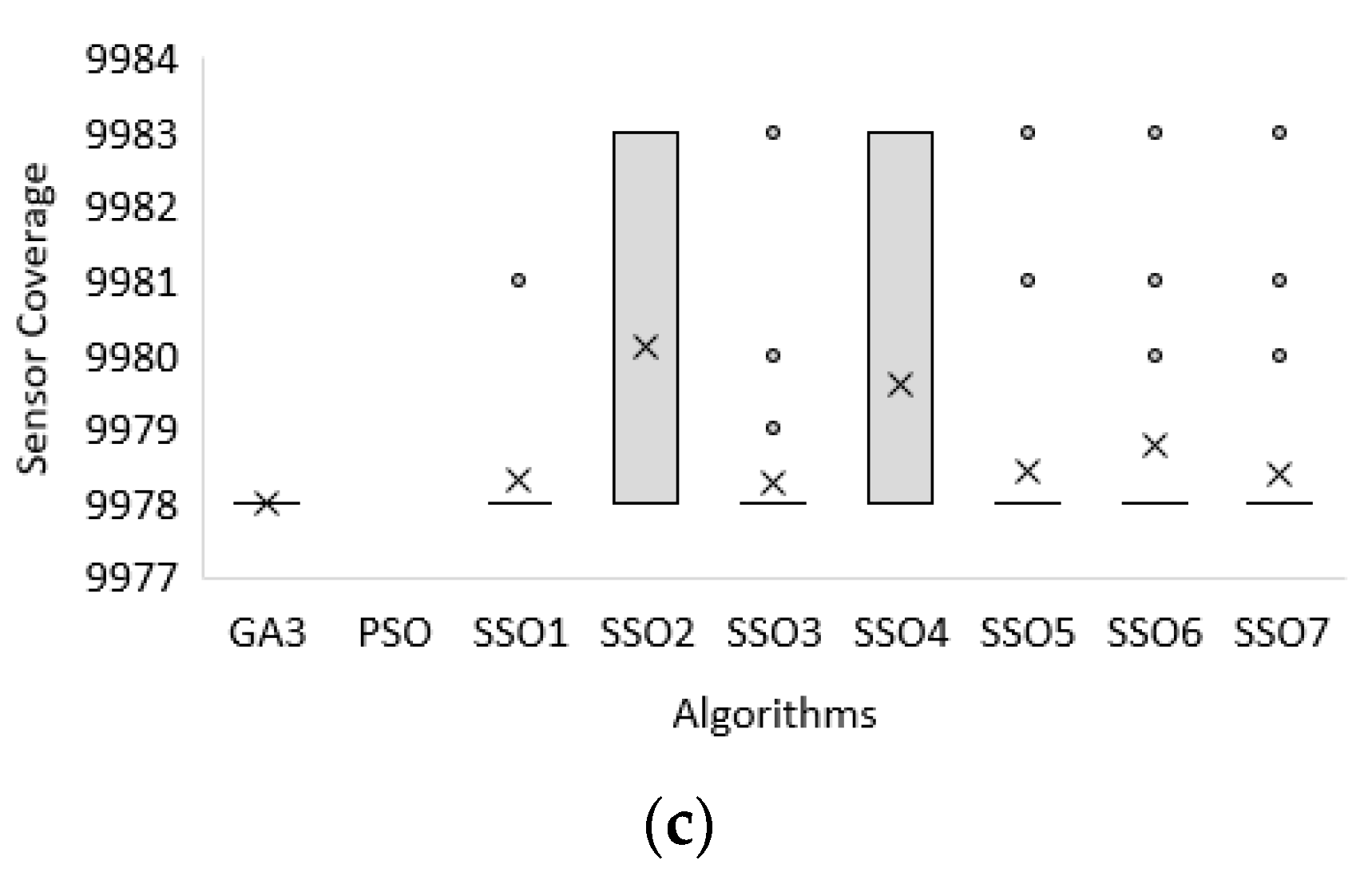
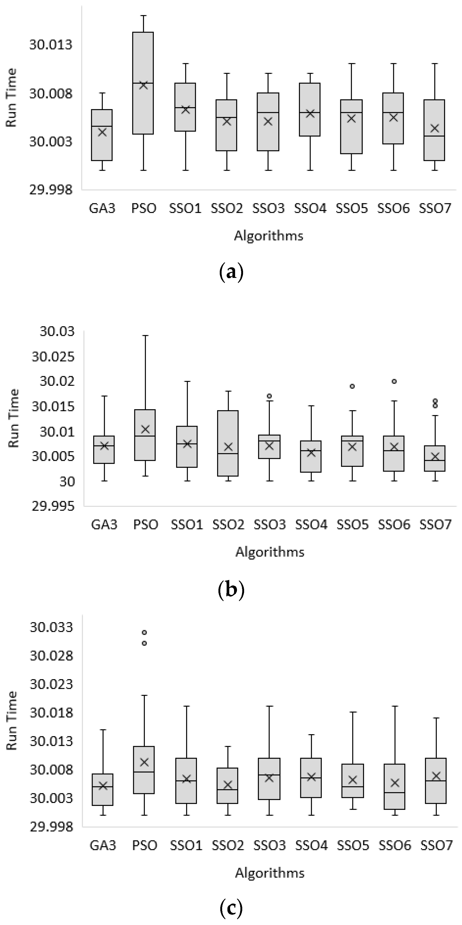
For a more abundant and detailed analysis of the experimental results, the statistical boxplots of the displayed images were adopted to show the performance including the maximum, interquartile range (75th percentile, median, and 25th percentile), and minimum and are shown in Figure 3, Figure 4, Figure 5, Figure 6, Figure 7 and Figure 8. Figure 3 and Figure 4 indicate the sensor coverage (fitness function value) and run time for all algorithms for the small-sized problem, Figure 5 and Figure 6 indicate the sensor coverage (fitness function value) and run time for all algorithms for the middle-sized problem, and Figure 7 and Figure 8 indicate the sensor coverage (fitness function value) and run time for all algorithms for the larger-sized problem, respectively.

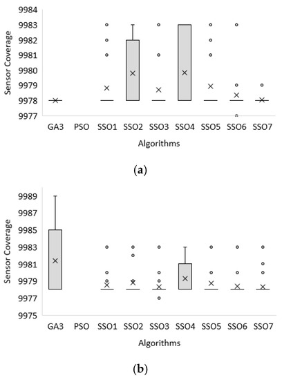
Figure 3. Boxplot of the sensor coverage (fitness function value) among all algorithms for the small-sized problem. (a) The first dataset. (b) The second dataset. (c) The third dataset.

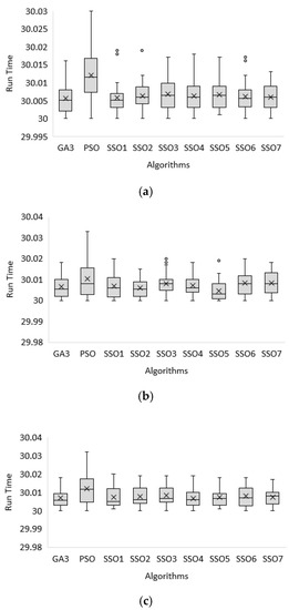
Figure 4. Boxplot of the run time among all algorithms for the small-sized problem. (a) The first dataset. (b) The second dataset. (c) The third dataset.

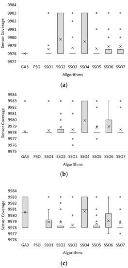
Figure 5. Boxplot of the sensor coverage (fitness function value) among all algorithms for the middle-sized problem. (a) The first dataset. (b) The second dataset. (c) The third dataset.

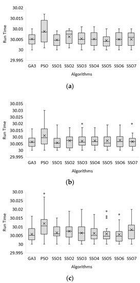
Figure 6. Boxplot of the run time among all algorithms for the middle-sized problem. (a) The first dataset. (b) The second dataset. (c) The third dataset.

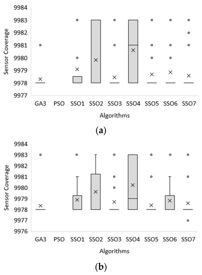
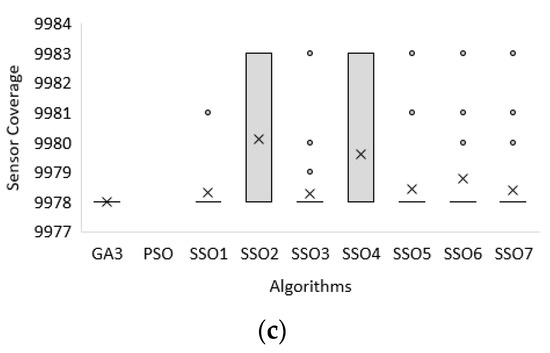
Figure 7. Boxplot of the sensor coverage (fitness function value) among all algorithms for the larger-sized problem. (a) The first dataset. (b) The second dataset. (c) The third dataset.

Figure 8. Boxplot of the run time among all algorithms for the larger-sized problem. (a) The first dataset. (b) The second dataset. (c) The third dataset.

Here, for the small-sized problem, the experimental results in terms of the fitness function of sensor coverage (F), the run time (T), the number of generations to obtain the optimal solution (Best), how many generations were run during the provided time (Ngen), and total cost (Cost) obtained by the GA, PSO, and the proposed bi-tuning SSO (SSO1–SSO7) are shown in Table 4, Table 5 and Table 6 and Figure 3 and Figure 4 and were analyzed as follows:

For the fitness function value (F):

• The best solution (MAX) of the fitness function value (F) obtained by SSO1-SSO6 is 9983, which is the best among all algorithms for the first dataset of the small-sized problem as shown in Table 4 and Figure 3a.
• The best solution (MAX) of the fitness function value (F) obtained by GA is 9989, which is the best among all algorithms for the second dataset of the small-sized problem as shown in Table 5 and Figure 3b.
• The best solution (MAX) of the fitness function value (F) obtained by SSO1-2 and SSO4-7 is 9983, which is the best among all algorithms for the third dataset of the small-sized problem as shown in Table 6 and Figure 3c.
• The average (AVG) of the fitness function value (F) was obtained by SSO4, GA. The AVG values in each database are 9979.83333, 9981.4, and 9979.36667, which are the best among all algorithms for the first dataset to the third dataset of the small-sized problem, respectively, as shown in Table 4, Table 5 and Table 6.
• The minimum (MIN) fitness function value (F) obtained by GA, SSO1-5, and SSO7 is 9978, which is the best among all algorithms for the first dataset of the small-sized problem, as shown in Table 4.
• The minimum (MIN) fitness function value (F) obtained by GA, SSO1-2, and SSO4-7 is 9978, which is the best among all algorithms for the second dataset to the third dataset of the small-sized problem, as shown in Table 5 and Table 6.
• The standard deviation (STD) values of the fitness function value (F) obtained by GA, SSO3, and GA are 0, 1.055364, and 0, which are the best among all algorithms for the first dataset to the third dataset of the small-sized problem, respectively, as shown in Table 4, Table 5 and Table 6.

For the run time (T):

• The best solution (MAX), average (AVG), and minimum (MIN) run time (T) obtained by all 9 algorithms is around 30 s for the first dataset to the third dataset of the small-sized problem, respectively, as shown in Table 4, Table 5 and Table 6.
• If it is compared more accurately, the best solution (MAX) for the run time (T) obtained by PSO shows the worst performance because it has the longest time for the first dataset to the third dataset of the small-sized problem, respectively, as shown in Table 4, Table 5 and Table 6 and Figure 4.

For the number of generations obtains the optimal solution (Best):

• The average (AVG) number of generations to obtain the optimal solution (Best) obtained by PSO is around 1 for the first dataset to the third dataset of the small-sized problem, respectively, as shown in Table 4, Table 5 and Table 6. In the same run time, the PSO converges faster but the solution is not better, which indicates it is trapped in the local solution and cannot escape.

For how many generations were run during the provided time (Ngen):

• The best solutions (MAX) of how many generations were run during the provided time (Ngen) obtained by GA are 3018, 2959, and 3021, which are the best among all algorithms for the first dataset to the third dataset of the small-sized problem, respectively, as shown in Table 4, Table 5 and Table 6.
• The proposed SSO1–SSO7 are the updates of all variables, showing that the average run time of each generation is long. In the future, it will be changed to the update of some variables.

For the total cost (Cost):

• The best solution (MAX) values of the total cost (Cost) obtained by PSO are 2197, 2182, and 2200, which exceed the cost limit of 2000 for the first dataset to the third dataset of the small-sized problem, respectively, as shown in Table 4, Table 5 and Table 6.
• The total cost obtained by GA and the proposed SSO1–SSO7 comply with the cost limit of 2000 for the first dataset to the third dataset of the small-sized problem, respectively, as shown in Table 4, Table 5 and Table 6.

Secondly, for the middle-sized problem, the experimental results in terms of the fitness function value (F), the run time (T), the number of generations to obtain the optimal solution (Best), how many generations were run during the provided time (Ngen), and total cost (Cost) obtained by the GA, PSO, and the proposed bi-tuning SSO (SSO1–SSO7) are shown in Table 7, Table 8 and Table 9 and Figure 5 and Figure 6 and were analyzed as follows:

For the fitness function value (F):

• The best solution (MAX) of the fitness function value (F) obtained by SSO1–SSO7 is 9983, which is the best among all algorithms for the first dataset of the middle-sized problem as shown in Table 7 and Figure 5a.
• The best solution (MAX) of the fitness function value (F) obtained by GA and SSO1–SSO7 is 9983, which is the best among all algorithms for the second dataset to the third dataset of the middle-sized problem as shown in Table 8 and Table 9 and Figure 5b,c.
• The average (AVG) fitness function values (F) obtained by SSO2, SSO4, and SSO4 are 9979.767, 9979.9, and 9980.633, which are the best among all algorithms for the first dataset to the third dataset of the middle-sized problem, respectively, as shown in Table 7, Table 8 and Table 9.
• The minimum (MIN) fitness function value (F) obtained by GA, SSO1–7 is 9978, which is the best among all algorithms for the first dataset of the middle-sized problem, as shown in Table 7.
• The minimum (MIN) fitness function value (F) obtained by GA, SSO1-2, SSO4, and SSO6-7 is 9978, which is the best among all algorithms for the second dataset of the middle-sized problem, as shown in Table 8.
• The minimum (MIN) fitness function value (F) obtained by GA and SSO1-5 is 9978, which is the best among all algorithms for the third dataset of the middle-sized problem, as shown in Table 9.
• The standard deviation (STD) values of the fitness function value (F) obtained by GA, GA, and SSO3 are 0, 0.912871, and 1.302517, which are the best among all algorithms for the first dataset to the third dataset of the middle-sized problem, respectively, as shown in Table 7, Table 8 and Table 9.

For the run time (T):

• The best solution (MAX), average (AVG), and minimum (MIN) for the run time (T) obtained by all 9 algorithms are around 30 s for the first dataset to the third dataset of the middle-sized problem, respectively, as shown in Table 7, Table 8 and Table 9.
• If it is compared more accurately, the best solution (MAX) for the run time (T) obtained by PSO shows the worst performance because it has the longest time for the first dataset to the third dataset of the middle-sized problem, respectively, as shown in Table 7, Table 8 and Table 9 and Figure 6.

For the number of generations to obtain the optimal solution (Best):

• The average (AVG) number of generations to obtain the optimal solution (Best) obtained by PSO is around 1 for the first dataset to the third dataset of the middle-sized problem, respectively, as shown in Table 7, Table 8 and Table 9. In the same run time, the PSO converges faster but the solution is not better, which indicates it is trapped in the local solution and cannot escape.

For how many generations were run during the provided time (Ngen):

• The best solution (MAX) for how many generations were run during the provided time (Ngen) obtained by GA are 3084, 2909, and 2974, which are the best among all algorithms for the first dataset to the third dataset of the middle-sized problem, respectively, as shown in Table 7, Table 8 and Table 9.
• The proposed SSO1–SSO7 represent the update of all variables, meaning that the average run time of each generation is long. In the future, it will be changed to the update of some variables.

For the total cost (Cost):

• The best solution (MAX) values of the total cost (Cost) obtained by PSO are 2165, 2189, and 2172, which exceed the cost limit of 2000 for the first dataset to the third dataset of the middle-sized problem, respectively, as shown in Table 7, Table 8 and Table 9.
• The total cost obtained by GA and the proposed SSO1–SSO7 comply with the cost limit of 2000 for the first dataset to the third dataset of the middle-sized problem, respectively, as shown in Table 7, Table 8 and Table 9.

Finally, for the larger-sized problem, the experimental results in terms of the fitness function value (F), the run time (T), the number of generations to obtain the optimal solution (Best), how many generations were run during the provided time (Ngen), and total cost (Cost) obtained by the GA, PSO, and the proposed bi-tuning SSO (SSO1–SSO7) are shown in Table 10, Table 11 and Table 12 and Figure 7 and Figure 8 and were analyzed as follows:

For the fitness function value (F):

• The best solution (MAX) of the fitness function value (F) obtained by SSO1–SSO7 is 9983, which is the best among all algorithms for the first dataset of the larger-sized problem as shown in Table 10 and Figure 7a.
• The best solution (MAX) of the fitness function value (F) obtained by GA and SSO1–SSO7 is 9983, which is the best among all algorithms for the second dataset of the larger-sized problem as shown in Table 11 and Figure 7b.
• The best solution (MAX) of the fitness function value (F) obtained by SSO2-SSO7 is 9983, which is the best among all algorithms for the third dataset of the larger-sized problem as shown in Table 12 and Figure 7c.
• The average (AVG) fitness function values (F) obtained by SSO4, SSO4, and SSO2 are 9980.6, 9980.233, and 9980.1, which are the best among all algorithms for the first dataset to the third dataset of the larger-sized problem, respectively, as shown in Table 10, Table 11 and Table 12.
• The minimum (MIN) fitness function value (F) obtained by GA and SSO1-7 is 9978, which is the best among all algorithms for the first dataset and the third dataset of the larger-sized problem, as shown in Table 10 and Table 12.
• The minimum (MIN) fitness function value (F) obtained by GA and SSO1-6 is 9978, which is the best among all algorithms for the second dataset of the larger-sized problem, as shown in Table 11.
• The standard deviation (STD) values of the fitness function value (F) obtained by GA, SSO5, and GA are 0.915386, 1.159171, and 0, which are the best among all algorithms for the first dataset to the third dataset of the larger-sized problem, respectively, as shown in Table 10, Table 11 and Table 12.

For the run time (T):

• The best solution (MAX), average (AVG), and minimum (MIN) of the run time (T) obtained by all 9 algorithms are around 30 s for the first dataset to the third dataset of the larger-sized problem, respectively, as shown in Table 10, Table 11 and Table 12.
• If it is compared more accurately, the best solution (MAX) of the run time (T) obtained by PSO shows the worst performance because it has the longest time for the first dataset to the third dataset of the larger-sized problem, respectively, as shown in Table 10, Table 11 and Table 12 and Figure 8.

For the number of generations to obtain the optimal solution (Best):

• The average (AVG) number of generations to obtain the optimal solution (Best) obtained by PSO is around 1 for the first dataset to the third dataset of the larger-sized problem, respectively, as shown in Table 10, Table 11 and Table 12. In the same run time, the PSO converges faster but the solution is not better, which indicates it is trapped in the local solution and cannot escape.

For how many generations were run during the provided time (Ngen):

• The best solution (MAX) values of how many generations were run during the provided time (Ngen) obtained by GA are 3140, 2864, and 2959, which are the best among all algorithms for the first dataset to the third dataset of the larger-sized problem, respectively, as shown in Table 10, Table 11 and Table 12.
• The proposed SSO1–SSO7 represent the update of all variables, meaning that the average run time of each generation is long. In the future, it will be changed to the update of some variables.

For the total cost (Cost):

• The best solution (MAX) values of the total cost (Cost) obtained by PSO are 2196, 2187, and 2191, which exceed the cost limit 2000 for the first dataset to the third dataset of the larger-sized problem, respectively, as shown in Table 10, Table 11 and Table 12.
• The total cost obtained by GA and the proposed SSO1–SSO7 comply with the cost limit of 2000 for the first dataset to the third dataset of the larger-sized problem, respectively, as shown in Table 10, Table 11 and Table 12.

Therefore, a more streamlined summary from the above analysis is shown as follows.

For the small-sized problem, the experimental results obtained by the proposed bi-tuning SSO outperform those found by PSO, GA, and SSO in terms of the fitness function of the sensor coverage (F) for the first dataset and the third dataset and comply with the cost limit of 2000 for the first dataset to the third dataset.

For the middle-sized problem and larger-sized problem, the experimental results obtained by the proposed bi-tuning SSO outperform those found by PSO, GA, and SSO in terms of the fitness function of the sensor coverage (F) for the first dataset to the third dataset and comply with the cost limit of 2000 for the first dataset to the third dataset.

Thus, the experimental results obtained by the proposed bi-tuning SSO achieve an excellent performance in terms of the fitness function of the sensor coverage (F) and comply with the cost limit of 2000 for all size problems including the small-sized, middle-sized, and larger-sized problems.

7. Conclusions

The WSN reveals a major system of wireless environments for many application systems in the modern world. In this study, a budget-limited WSN sensing coverage problem was considered. To enhance the QoS in WSN, the objective of the budget-limited WSN sensing coverage problem is to maximize the number of sensor coverage grids under the assumption that the number of sensors, the coverage radius level, the related cost of each sensor, and the budget limit are known.

This paper presented a new multi-objective swarm algorithm called the bi-tuning SSO including seven SSO variants (SSO1–SSO7) to optimize the solution of the studied problem in this paper. The proposed bi-tuning SSO was found to improve the SSO by tuning the parameter settings, which is always an important issue in all AI algorithms.

A comparative experiment of the effectiveness and performance of the proposed bi-tuning SSO algorithm was performed and compared to state-of-the-art algorithms including PSO and GA on three datasets with different settings of N_var = 20, 100, and 300, representing the scale of small, middle, and larger WSNs. The optimization solution obtained by all considered algorithms indicated the proposed bi-tuning SSO performs better than the compared algorithms from the best, the worst, the average, and standard deviation for the fitness function values obtained in all cases in this study. Given these outcomes, the proposed bi-tuning SSO should be extended, with future studies applying it to multi-class datasets with more attributes, classes, and instances.

References

- Wang, C.; Li, J.; Yang, Y.; Ye, F. Combining Solar Energy Harvesting with Wireless Charging for Hybrid Wireless Sensor Networks. IEEE Trans. Mob. Comput. 2018, 17, 560–576. [Google Scholar] [CrossRef]
- Yang, X.; Wang, L.; Su, J.; Gong, Y. Hybrid MAC Protocol Design for Mobile Wireless Sensors Networks. IEEE Sens. Lett. 2018, 2, 7500604. [Google Scholar] [CrossRef]
- Tolani, M.; Singh, R.K.; Shubham, K.; Kumar, R. Two-Layer Optimized Railway Monitoring System Using Wi-Fi and ZigBee Interfaced Wireless Sensor Network. IEEE Sens. J. 2017, 17, 2241–2248. [Google Scholar] [CrossRef]
- Daskalakis, S.N.; Goussetis, G.; Assimonis, S.D.; Tentzeris, M.M.; Georgiadis, A. A uW Backscatter-Morse-Leaf Sensor for Low-Power Agricultural Wireless Sensor Networks. IEEE Sens. J. 2018, 18, 7889–7898. [Google Scholar] [CrossRef] [Green Version]
- Wang, J.; Zhang, X. Cooperative MIMO-OFDM-Based Exposure-Path Prevention Over 3D Clustered Wireless Camera Sensor Networks. IEEE Trans. Wirel. Commun. 2020, 19, 4–18. [Google Scholar] [CrossRef]
- Sharma, D.; Bhondekar, A.P. Traffic and Energy Aware Routing for Heterogeneous Wireless Sensor Networks. IEEE Commun. Lett. 2018, 22, 1608–1611. [Google Scholar] [CrossRef]
- Osamy, W.; Khedr, A.M.; Salim, A. ADSDA: Adaptive Distributed Service Discovery Algorithm for Internet of Things Based Mobile Wireless Sensor Networks. IEEE Sens. J. 2019, 19, 10869–10880. [Google Scholar] [CrossRef]
- Chen, S.; Zhang, L.; Tang, Y.; Shen, C.; Kumar, R.; Yu, K.; Tariq, U.; KashifBashir, A. Indoor Temperature Monitoring using Wireless Sensor Networks: A SMAC Application in Smart Cities. Sustain. Cities Soc. 2020, 61, 102333. [Google Scholar] [CrossRef]
- Kalaivaani, P.T.; Krishnamoorthi, R. Design and Implementation of Low Power Bio Signal Sensors for Wireless Body Sensing Network Applications. Microprocess. Microsyst. 2020, 79, 103271. [Google Scholar] [CrossRef]
- Huang, T.Y.; Chang, C.J.; Lin, C.W.; Roy, S.; Ho, T.Y. Delay-Bounded Intravehicle Network Routing Algorithm for Minimization of Wiring Weight and Wireless Transmit Power. IEEE Trans. Comput.-Aided Des. Integr. Circuits Syst. 2017, 36, 551–561. [Google Scholar] [CrossRef]
- Harbouche, A.; Djedi, N.; Erradi, M.; Ben-Othman, J.; Kobbane, A. Model Driven Flexible Design of a Wireless Body Sensor Network for Health Monitoring. Comput. Netw. 2017, 129, 548–571. [Google Scholar] [CrossRef]
- Kim, K.B.; Cho, J.Y.; Jeon, D.H.; Ahn, J.H.; Hong, S.D.; Jeong, Y.H.; Nahm, S.; Sung, T.H. RETRACTED: Enhanced Flexible Piezoelectric Generating Performance via High Energy Composite for Wireless Sensor Network. Energy 2018, 159, 196–202. [Google Scholar] [CrossRef]
- Munirathinam, K.; Park, J.; Jeong, Y.J.; Lee, D.W. Galinstan-Based Flexible Microfluidic Device for Wireless Human-Sensor Applications. Sens. Actuators A Phys. 2020, 315, 112344. [Google Scholar] [CrossRef]
- Haque, I.; Nurujjaman, M.; Harms, J.; Abu-Ghazaleh, N. SDSense: An Agile and Flexible SDN-Based Framework for Wireless Sensor Networks. IEEE Trans. Veh. Technol. 2019, 68, 1866–1876. [Google Scholar] [CrossRef]
- Kim, J.; Choi, J.P. Sensing Coverage-Based Cooperative Spectrum Detection in Cognitive Radio Networks. IEEE Sens. J. 2019, 19, 5325–5332. [Google Scholar] [CrossRef]
- Singh, P.; Chen, Y.C. Sensing Coverage Hole Identification and Coverage Hole Healing Methods for Wireless Sensor Networks. Wirel. Netw. 2020, 26, 2223–2239. [Google Scholar] [CrossRef]
- Huang, H.; Savkin, A.V.; Li, X. Reactive Autonomous Navigation of UAVs for Dynamic Sensing Coverage of Mobile Ground Targets. Sensors 2020, 20, 3720. [Google Scholar] [CrossRef]
- Chen, R.; Xu, N.; Li, J. A Self-Organized Reciprocal Decision Approach for Sensing Coverage with Multi-UAV Swarms. Sensors 2018, 18, 1864. [Google Scholar] [CrossRef] [Green Version]
- Wang, S.C.; Hsiao, H.C.W.; Lin, C.C.; Chin, H.H. Multi-Objective Wireless Sensor Network Deployment Problem with Cooperative Distance-Based Sensing Coverage. Mob. Netw. Appl. 2021, 134, 1–12. [Google Scholar] [CrossRef]
- Zhou, P.; Wang, C.; Yang, Y. Static and Mobile Target kk-Coverage in Wireless Rechargeable Sensor Networks. IEEE Trans. Mob. Comput. 2019, 18, 2430–2445. [Google Scholar] [CrossRef]
- Nguyen, N.T.; Liu, B.H. The Mobile Sensor Deployment Problem and the Target Coverage Problem in Mobile Wireless Sensor Networks are NP-Hard. IEEE Syst. J. 2019, 13, 1312–1315. [Google Scholar] [CrossRef]
- Alia, O.M.; Al-Ajouri, A. Maximizing Wireless Sensor Network Coverage with Minimum Cost Using Harmony Search Algorithm. IEEE Sens. J. 2017, 17, 882–896. [Google Scholar] [CrossRef]
- Dash, D. Approximation Algorithms for Road Coverage Using Wireless Sensor Networks for Moving Objects Monitoring. IEEE Trans. Intell. Transp. Syst. 2020, 21, 4835–4844. [Google Scholar] [CrossRef]
- Al-Karaki, J.N.; Gawanmeh, A. The Optimal Deployment, Coverage, and Connectivity Problems in Wireless Sensor Networks: Revisited. IEEE Access 2017, 5, 18051–18065. [Google Scholar] [CrossRef]
- Yu, J.; Wan, S.; Cheng, X.; Yu, D. Coverage Contribution Area Based k-Coverage for Wireless Sensor Networks. IEEE Trans. Veh. Technol. 2017, 66, 8510–8523. [Google Scholar] [CrossRef]
- Singh, S.; Kumar, S.; Nayyar, A.; Al-Turjman, F.; Mostarda, L. Proficient QoS-Based Target Coverage Problem in Wireless Sensor Networks. IEEE Access 2020, 8, 74315–74325. [Google Scholar]
- Yang, X.; Wen, Y.; Yuan, D.; Zhang, M.; Zhao, H.; Meng, Y. Coverage Degree-Coverage Model in Wireless Visual Sensor Networks. IEEE Wirel. Commun. Lett. 2019, 8, 817–820. [Google Scholar] [CrossRef]
- Elhoseny, M.; Tharwat, A.; Farouk, A.; Hassanien, A.E. K-Coverage Model Based on Genetic Algorithm to Extend WSN Lifetime. IEEE Sens. Lett. 2017, 1, 7500404. [Google Scholar] [CrossRef]
- Chakravarthi, S.S.; Kumar, G.H. Optimization of Network Coverage and Lifetime of the Wireless Sensor Network based on Pareto Optimization using Non-dominated Sorting Genetic Approach. Procedia Comput. Sci. 2020, 172, 225–228. [Google Scholar] [CrossRef]
- Jiao, Z.; Zhang, L.; Xu, M.; Cai, C.; Xiong, J. Coverage Control Algorithm-Based Adaptive Particle Swarm Optimization and Node Sleeping in Wireless Multimedia Sensor Networks. IEEE Access 2019, 7, 170096–170105. [Google Scholar] [CrossRef]
- Yeh, W.C. A two-stage discrete particle swarm optimization for the problem of multiple multi-level redundancy allocation in series systems. Expert Syst. Appl. 2009, 36, 9192–9200. [Google Scholar] [CrossRef]
- Yeh, W.C.; He, M.F.; Huang, C.L.; Tan, S.Y.; Zhang, X.; Huang, Y.; Li, L. New genetic algorithm for economic dispatch of stand-alone three-modular microgrid in DongAo Island. Appl. Energy 2020, 263, 114508. [Google Scholar] [CrossRef]
- Yeh, W.C.; Huang, C.L.; Lin, P.; Chen, Z.; Jiang, Y.; Sun, B. Simplex Simplified Swarm Optimization for the Efficient Optimization of Parameter Identification for Solar Cell Models. IET Renew. Power Gener. 2018, 12, 45–51. [Google Scholar] [CrossRef]
- Lin, P.; Cheng, S.; Yeh, W.C.; Chen, Z.; Wu, L. Parameters Extraction of Solar Cell Models Using a Modified Simplified Swarm Optimization Algorithm. Sol. Energy 2017, 144, 594–603. [Google Scholar] [CrossRef]
- Zhang, X.; Huang, Y.; Li, L.; Yeh, W.C. Power and Capacity Consensus Traking of Distributed Battery Storage Systems in Modular Microgrids. Energies 2018, 11, 1439. [Google Scholar] [CrossRef] [Green Version]
- Huang, C.L.; Yin, Y.; Jiang, Y.; Yeh, W.C.; Chung, Y.Y.; Lai, C.M. Multi-objective Scheduling in Cloud Computing using MOSSO. In Proceedings of the 2018 IEEE Congress on Evolutionary Computation (CEC 2018), Rio de Janeiro, Brazil, 8–13 July 2018. [Google Scholar]
- Lai, C.M.; Yeh, W.C.; Huang, Y.C. Entropic Simplified Swarm Optimization for the Task Assignment Problem. Appl. Soft Comput. 2017, 58, 115–127. [Google Scholar] [CrossRef]
- Yeh, W.C.; Lai, C.-M.; Huang, Y.-C.; Cheng, T.-W.; Huang, H.-P.; Jiang, Y. Simplified Swarm Optimization for Task Assignment Problem in Distributed Computing System. In Proceedings of the 2017 13th International Conference on Natural Computation, Fuzzy Systems and Knowledge Discovery (ICNC-FSKD 2017), Guilin, China, 29–31 July 2017. [Google Scholar]
- Yeh, W.C.; Lin, J.S. New parallel swarm algorithm for smart sensor systems redundancy allocation problems in the Internet of Things. J. Supercomput. 2018, 74, 4358–4384. [Google Scholar] [CrossRef]
- Yeh, W.C. A Hybrid Heuristic Algorithm for the Multistage Supply Chain Network Problem. Int. J. Adv. Manuf. Technol. 2005, 26, 675–685. [Google Scholar] [CrossRef]
- Yeh, W.C. Simplified Swarm Optimization in Disassembly Sequencing Problems with Learning Effects. Comput. Oper. Res. 2012, 39, 2168–2177. [Google Scholar] [CrossRef]
- Yeh, W.C.; Jiang, Y.; Huang, C.L.; Xiong, N.N.; Hu, C.F.; Yeh, Y.H. Improve Energy Consumption and Signal Transmission Quality of Routings in Wireless Sensor Networks. IEEE Access 2020, 8, 198254–198264. [Google Scholar] [CrossRef]
- Hsieh, J.; Hsiao, H.F.; Yeh, W.C. Forecasting Stock Markets Using Wavelet Transforms and Recurrent Neural Networks: An Integrated System Based on Artificial Bee Colony Algorithm. Appl. Soft Comput. 2011, 11, 2510–2525. [Google Scholar] [CrossRef]
- Chakraborty, S.; Goyal, N.K.; Soh, S. On Area Coverage Reliability of Mobile Wireless Sensor Networks with Multistate Nodes. IEEE Sens. J. 2020, 20, 4992–5003. [Google Scholar] [CrossRef]
- Zhang, L.; Liu, T.T.; Wen, F.Q.; Hu, L.; Hei, C.; Wang, K. Differential Evolution Based Regional Coverage-Enhancing Algorithm for Directional 3D Wireless Sensor Networks. IEEE Access 2019, 7, 93690–93700. [Google Scholar] [CrossRef]
- Han, G.; Liu, L.; Jiang, J.; Shu, L.; Hancke, G. Analysis of Energy-Efficient Connected Target Coverage Algorithms for Industrial Wireless Sensor Networks. IEEE Trans. Ind. Inform. 2017, 13, 135–143. [Google Scholar] [CrossRef]
- Yeh, W.C.; Tan, S.Y. Simplified Swarm Optimization for the Heterogeneous Fleet Vehicle Routing Problem with Time-Varying Continuous Speed Function. Electronics 2021, 10, 1775. [Google Scholar] [CrossRef]
- Yeh, W.C.; Su, Y.Z.; Gao, X.Z.; Hu, C.F.; Wang, J.; Huang, C.L. Simplified Swarm Optimization for Bi-Objection Active Reliability Redundancy Allocation Problems. Appl. Soft Comput. J. 2021, 106, 107321. [Google Scholar] [CrossRef]
- Yeh, W.C. Solving cold-standby reliability redundancy allocation problems using a new swarm intelligence algorithm. Appl. Soft Comput. 2019, 83, 105582. [Google Scholar] [CrossRef]
- Wang, M.; Yeh, W.C.; Chu, T.C.; Zhang, X.; Huang, C.L.; Yang, J. Solving Multi-Objective Fuzzy Optimization in Wireless Smart Sensor Networks under Uncertainty Using a Hybrid of IFR and SSO Algorithm. Energies 2018, 11, 2385. [Google Scholar] [CrossRef] [Green Version]
- Huang, C.L.; Jiang, Y.; Yeh, W.C. Developing Model of Fuzzy Constraints Based on Redundancy Allocation Problem by an Improved Swarm Algorithm. IEEE Access 2020, 8, 155235–155247. [Google Scholar] [CrossRef]
- Lai, C.M.; Chiu, C.C.; Liu, W.C.; Yeh, W.C. A novel nondominated sorting simplified swarm optimization for multi-stage capacitated facility location problems with multiple quantitative and qualitative objectives. Appl. Soft Comput. 2019, 84, 105684. [Google Scholar] [CrossRef]
- Yeh, W.C. A new harmonic continuous simplified swarm optimization. Appl. Soft Comput. 2019, 85, 105544. [Google Scholar] [CrossRef]
- Zhu, W.; Yeh, W.C.; Cao, L.; Zhu, Z.; Chen, D.; Chen, J.; Li, A.; Lin, Y. Faster Evolutionary Convolutional Neural Networks Based on iSSO for Lesion Recognition in Medical Images. Basic Clin. Pharmacol. Toxicol. 2019, 124, 329. [Google Scholar]
- Huang, C.L.; Huang, S.Y.; Yeh, W.C.; Wang, J. Fuzzy System and Time Window Applied to Traffic Service Network Problem under Multi-demand Random Network. Electronics 2019, 8, 539. [Google Scholar] [CrossRef] [Green Version]
- Sun, L.; Zhu, W.; Lu, Q.; Li, A.; Luo, L.; Chen, J.; Wang, J. CellNet: An Improved Neural Architecture Search Method for Coal and Gangue Classification. In Proceedings of the IJCNN 2021: International Joint Conference on Neural Networks, Shenzhen, China, 18–22 July 2021. [Google Scholar]
- Jin, H.; Zhu, W.; Duan, Z.; Chen, J.; Li, A. TDNN-LSTM Model and Application Based on Attention Mechanism. Acoust. Technol. 2021, 40, 508–514. [Google Scholar]
- Zhu, W.; Ma, H.; Cai, G.; Chen, J.; Wang, X.; Li, A. Research on PSO-ARMA-SVR Short-Term Electricity Consumption Forecast Based on the Particle Swarm Algorithm. Wirel. Commun. Mob. Comput. 2021, 2021, 6691537. [Google Scholar]
- Zhu, W.; Yeh, W.C.; Xiong, N.N.; Sun, B. A New Node-based Concept for Solving the Minimal Path Problem in General networks. IEEE Access 2019, 7, 173310–173319. [Google Scholar] [CrossRef]
- Zhu, W.; Yeh, W.C.; Chen, J.; Chen, D.; Li, A.; Lin, Y. Evolutionary convolutional neural networks using ABC. In Proceedings of the 2019 11th International Conference on Machine Learning and Computing (ICMLC 2019), Zhuhai, China, 22–24 February 2019. [Google Scholar]
- Yeh, W.C. A new branch-and-bound approach for the n/2/flowshop/αF+ βCmax flowshop scheduling problem. Comput. Oper. Res. 1999, 26, 1293–1310. [Google Scholar] [CrossRef]
- Zhang, Y.; Wang, G.G.; Li, K.; Yeh, W.C.; Jian, M.; Dong, J. Enhancing MOEA/D with information feedback models for large-scale many-objective optimization. Inf. Sci. 2020, 522, 1–16. [Google Scholar] [CrossRef]
- Corley, H.W.; Rosenberger, J.; Yeh, W.C.; Sung, T.K. The cosine simplex algorithm. Int. J. Adv. Manuf. Technol. 2006, 27, 1047–1050. [Google Scholar] [CrossRef]
Publisher’s Note: MDPI stays neutral with regard to jurisdictional claims in published maps and institutional affiliations. |
© 2021 by the authors. Licensee MDPI, Basel, Switzerland. This article is an open access article distributed under the terms and conditions of the Creative Commons Attribution (CC BY) license (https://creativecommons.org/licenses/by/4.0/).