Design General Cam Profiles Based on Finite Element Method

Abstract

This paper presents a general framework to design a cam profile using the finite element method from given displacements of the follower. The arbitrarily complex cam profile is described by Lagrangian finite elements, which are formed by the connectivity of nodes. In order to obtain the desired profile, a penalty-type functional that enforces the prescribed displacement of the follower is proposed. Additionally, in order to ensure convexity of the functional, a numerical stabilization scheme is used. The nodal positions are then obtained by solving a nonlinear system of equations resulting from minimizing the total functional. The geometrical accuracy of the cam profile can be controlled by the number of finite elements. A case study is considered to illustrate the flexibility, accuracy, and robustness of the proposed approach.

1. Introduction

Cam mechanisms are widely used in various mechanical machines, such as machine tools, sewing machines, and engines due to their unlimited motions, operation speed, motion accuracy, and structural rigidity. In cam design, the follower motion affects the kinematic and dynamic characteristics of cam systems. Various traditional functions can be used to describe the follower motion such as harmonic, cycloidal, trapezoidal, polynomial, and piecewise polynomial [1,2]. So far, spline functions have also been used to develop the cam curves, for example, the Bezier curve [3], the B-spline curve [4,5,6], and the NURBS curve [7,8,9,10]. Besides, kinematics and dynamics have been considered to optimize the peak values of the displacement, velocity, acceleration, and jerk with referring to several functions, e.g., harmonic, cycloidal, and polynomial [11]. Qin and Chen [12] also proposed the kinematic optimization of cam motions for engine valve trains regarding the characteristics of polynomial cam curves. In order to achieve motion curves with good dynamic characteristics under arbitrary design conditions, the parameters of the motion model were obtained by optimizing the dynamic performance [13,14]. Related to the cam design process, the cam size optimization has been also investigated [15,16,17]. This plays an important role due to affect the cost of cam systems.

The design of the cam profile is one of the main tasks in designing a cam mechanism. The profile of the cam must be designed correctly to ensure the characteristics of kinematics and dynamics of cam mechanisms. However, when a priori displacement of the follower is given, obtaining the corresponding curve equations for cam profiles is nontrivial in general. Many approaches to design the profile of a cam have been proposed. The graphical method has been established by several studies for disk cams [1,18,19]. In this method, kinematic inversion is used. To increase the accuracy, the analytical method using a Cartesian coordinate system is presented by [20,21,22]. Since then, the analytical method has been continuously advanced, among others by Shigley and Jr. [1] and Norton [23]. In these studies, the equations of cam profile have been formulated by the loop-closure equation and using complex polar notation. Wu et al. [24] presented a cam profile of a translating cam driven. In this approach, the follower motion can be arbitrarily chosen for only the forward or the return stroke. The desired cam profile is obtained by using the theory of envelopes [25]. To this end, the envelopes are given by fitting a tangent curve to the successive follower positions, and the cam profile is achieved by the boundary of the family. Biswas et al. [26] presented two approximate analytical methods for determining disk cam profiles of roller followers. In the first method, the average location is defined by two lines tangent of three roller positions. The cam profile is obtained by the interpolation of the roller positions. In the second method of this research, the cam profile is achieved by the intersection of the curvature center and the roller center. A systematic method for the design and analysis of cams with three circular-arc profiles is presented by Jung-Fa Hsieh [27]. This study is based on constructing a generic geometric model of cam profile and deriving the corresponding equations of the constituent circular arcs using a coordinate transformation. Moreover, using coordinate transformation, the cam profile is obtained by [28]. This study proposes a simple yet comprehensive method for the design and analysis of an indexing cam mechanism with parallel axes.

In this paper, we propose a finite element method to design a cam profile from a given displacement of the follower. To the best of our knowledge, this is the first time a finite element description is used directly for obtaining the cam profile. Compared to earlier works, the presented method contains the following merits and novelties:

• A penalty type functional to enforce the prescribed displacement of the follower is proposed;
• A stabilization scheme is added to guarantee convexity of the functional;
• For the Newton–Raphson solution method, the consistent linearization of the weak form is presented;
• The arbitrary desired accuracy of the cam profile can be achieved by increasing the number of finite elements;
• The resulting profile represented by finite elements can be used for cam manufacturing.

The remainder of the paper is structured as follows. In Section 2, the geometrical description of cam profiles is presented. Section 3 introduces the synthetical kinematics. The formulation of the general framework for the synthesis of cam mechanisms is presented in Section 4. The finite element (FE) formulation is discussed in Section 5. Section 6 then presents a solution of the finite element. The case study for this method is presented in Section 7. Finally, conclusions are drawn in Section 8.

2. Geometrical Description of Cam Profiles

In this section, we present the geometrical description of the cam profile. The differential geometry (see [29]) is used for an arbitrarily complex cam surface. The cam surface, denoted by $S$ (see Figure 1), is represented in curvilinear coordinates as

$$\begin{array}{c}\mathit{x}=\mathit{x}\left(\mathbf{\xi }\right) ,\end{array}$$

(1)

where $\mathsf{\xi } \left({\mathsf{\xi }}^1,{\mathsf{\xi }}^2\right)$ are the curvilinear coordinates. Accordingly, the covariant and contravariant tangent vectors, $a_{\mathsf{\alpha }} \mathrm{and} a^{\mathsf{\alpha }}$, at point $\mathit{x}$ depending on S are calculated by

$$\begin{array}{cc}{a}_{\mathsf{\alpha }}=\frac{\partial \mathit{x}}{\partial {\mathsf{\xi }}^{\mathsf{\alpha }}}& ,\end{array}$$

(2)

and

$$\begin{array}{c}{a}^{\mathsf{\alpha }}:={ \mathrm{a}}^{\mathsf{\alpha }\mathsf{\beta }} a_{\mathsf{\beta }} ,\end{array}$$

(3)

respectively, where

$$\begin{gathered} \begin{array}{c}{\mathrm{a}}^{\mathsf{\alpha }\mathsf{\beta }}:={\left[{\mathrm{a}}_{\mathsf{\alpha }\mathsf{\beta }}\right]}^{-1},\end{array} \\ {\mathrm{a}}_{\mathsf{\alpha }\mathsf{\beta }}:= a_{\mathsf{\alpha }}· a_{\mathsf{\beta }} \end{gathered}$$

(4)

are the contravariant and covariant components of the metric tensor. Here and henceforth, the summation convention is implied for repeated Greek indices, e.g., $\alpha$ = 1, 2. The unit normal vector $n$ at $\mathit{x}$ is defined by [30]

$$\begin{array}{cc}n=\frac{ a_1\times a_2}{\Vert a_1\times a_2\Vert }& .\end{array}$$

(5)

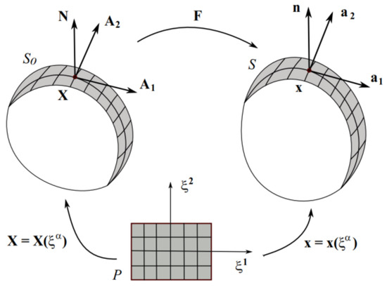
Figure 1. Mapping between parameter domain P, reference configuration S₀, and current configuration S.

It can be shown that

$$\Vert a_1\times a_2\Vert =\sqrt{\det {\mathrm{a}}_{\mathsf{\alpha }\mathsf{\beta }}} .$$

(6)

The curvature tensor can be computed as (see, e.g., [29])

$$b={ \mathrm{b}}_{\mathsf{\alpha }\mathsf{\beta }} a^{\mathsf{\alpha }}\otimes a^{\mathsf{\beta }},$$

(7)

where

$${\mathrm{b}}_{\mathsf{\alpha }\mathsf{\beta }}:=n · a_{\mathsf{\alpha },\mathsf{\beta }} .$$

(8)

3. Synthetical Kinematics

In this section, the established approach to describe the deformation of membranes (see, e.g., [29]) is employed in the context of synthetical kinematics for designing cam profiles. To obtain the desired cam profile, a given initial configuration is selected. The initial curve is then “deformed” to the desired configuration. The differences between the initial (reference) configuration $S_0$ and the current configuration $S$ are shown in Figure 1. Both configurations are described by the geometrical quantities discussed in Section 2. For the reference configuration $S_0$ we use the upper-case symbols $\mathit{X}$, $A_{\mathsf{\alpha }}$, ${\mathrm{A}}_{\mathsf{\alpha }\mathsf{\beta }}$, $A^{\mathsf{\alpha }}$, and $N$. The corresponding lower-case symbols $\mathit{x}$, $a_{\mathsf{\alpha }}$, ${\mathrm{a}}_{\mathsf{\alpha }\mathsf{\beta }}$, $a^{\mathsf{\alpha }}$, and $n$ are used in the current configuration $S$. In order to characterize the deformation between the reference configuration $S_0$ and the current configuration $S$, a line element in $S$ is considered as

$$\mathrm{d}\mathit{x}=a_{\mathsf{\alpha }} \mathrm{d}{\mathsf{\xi }}^{\mathsf{\alpha }},$$

(9)

and its corresponding line $\mathrm{d}\mathit{X}=A_{\mathsf{\alpha }}\mathrm{d}{\mathsf{\xi }}^{\mathsf{\alpha }}$ in $S_0$. So that we can write $\mathrm{d}{\mathsf{\xi }}^{\mathsf{\alpha }}=A^{\mathsf{\alpha }}\mathrm{d}\mathit{X}$. With this, $\mathrm{d}\mathit{x}$ in the current configuration can be mapped to $\mathrm{d}\mathit{X}$ in $S_0$ by

$$\mathrm{d}\mathit{x}=\left(a_{\alpha }\otimes A^{\alpha }\right)\mathrm{d}\mathit{X}.$$

(10)

Here the tensor

$$F=a_{\mathsf{\alpha }}\otimes A^{\mathsf{\alpha }}$$

(11)

denotes the deformation gradient. Vice versa

$$F^{-1}=A_{\mathsf{\alpha }}\otimes a^{\mathsf{\alpha }}$$

(12)

maps the $\mathrm{d}\mathit{X}$ in $S_0$ to $\mathrm{d}\mathit{x}$ in $S$. Through F we thus have the following transformation

$$\begin{gathered} a_{\mathsf{\alpha }}=F A_{\mathsf{\alpha }}, A_{\mathsf{\alpha }}=F^{-1}{a}_{\mathsf{\alpha }} , \\ {a}^{\mathsf{\alpha }}=F^{-\mathrm{T}}{A}^{\mathsf{\alpha }}, A^{\mathsf{\alpha }}=F^{\mathrm{T}} a^{\mathsf{\alpha }}. \end{gathered}$$

(13)

Finally, the stretch between configurations $S_0$ and $S$ is defined by

$$\begin{gathered} \mathrm{J}:=\frac{{\mathrm{J}}_{\mathrm{a}}}{{ \mathrm{J}}_{\mathrm{A}}} , \\ { \mathrm{J}}_{\mathrm{A}}:=\sqrt{{\det \mathrm{A}}_{\mathsf{\alpha }\mathsf{\beta }}} , \\ { \mathrm{J}}_{\mathrm{a}}:=\sqrt{{\det \mathrm{a}}_{\mathsf{\alpha }\mathsf{\beta }}} . \end{gathered}$$

(14)

Here, “det” denotes the surface determinant.

4. Governing Equation for the Synthesis of Cam Profile

In this section, the governing equation for designing cam profile is proposed. The strong form, weak form, and stabilization scheme are presented.

4.1. Strong form Statement

The point-wised governing equation for the synthesis of cam profile is given by

$$\mathrm{g}:=\mathrm{s}-{\mathrm{s}}_0=0,\forall \mathit{x} \in \mathrm{S} ,$$

(15)

subjected to the boundary condition

$$\mathit{x}=\overline{\mathit{x}},\forall \mathit{x} \in {\mathrm{\Gamma }}_{\mathrm{u}} ,$$

(16)

where ${\mathrm{s}}_0$ and $\mathrm{s}$ denote the reference and current displacement of the follower, respectively. ${\mathrm{s}}_0$ and $\mathrm{s}$ will be explicitly defined for a particular type of cam. ${\mathrm{\Gamma }}_{\mathrm{u}}$ is a subset of $\mathrm{S}$. From Equation (15), the variation $\mathrm{\delta }\mathrm{g}$ can be expressed as

$$\mathrm{\delta }\mathrm{g}=\mathrm{\delta }\mathrm{s}-{\mathrm{\delta }\mathrm{s}}_0 ,$$

(17)

where

$$\begin{array}{cc}\mathrm{\delta }\mathrm{s}=\frac{\partial \mathrm{s}}{\partial \mathit{x}}·\mathrm{\delta }\mathit{x} , & {\mathrm{\delta }\mathrm{s}}_0=\frac{\partial {\mathrm{s}}_0}{\partial \mathit{x}}·\mathrm{\delta }\mathit{x}\end{array} .$$

(18)

The strong form equation as shown in Equations (15) and (16) is not a well-posed statement since it is still missing an in-plane constraint equation. In another word, the positions of two arbitrary material points ${\mathit{x}}_1\in S\backslash {\mathrm{\Gamma }}_{\mathrm{u}}$ and ${\mathit{x}}_2\in S\backslash {\mathrm{\Gamma }}_{\mathrm{u}}$ can be exchanged without affecting the solution of Equation (15). The system is thus unstable and needs stabilization, which will be discussed in Section 4.4.

4.2. Penalty-Type Functional

The point-wise condition in Equation (15) can be enforced by a penalty-type functional. The penalty-type functional can be expressed as

$${\mathrm{\Pi }}_{\mathrm{p}}={{\displaystyle \int }}_{S_0}\frac{\mathrm{ϵ}}{2}{\mathrm{g}}^2{ \mathrm{dA}}_0 ,$$

(19)

where $\mathrm{ϵ}$ is the penalty parameter. The variation of the penalty-type functional is computed as

$$\mathrm{\delta }{\mathrm{\Pi }}_{\mathrm{p}}={{\displaystyle \int }}_{S_0}{\mathsf{\lambda } \mathrm{\delta }\mathrm{g} \mathrm{dA}}_0 ,$$

(20)

where

$$\mathsf{\lambda }:=\mathrm{ϵ} \mathrm{g}$$

(21)

represents the pressure of the enforcement.

It should be noted that the potential in Equation (19) exactly enforces the condition at the limit, i.e., $\mathrm{ϵ}\to \infty$. At $\mathrm{ϵ}\to 0$, ${\mathrm{\Pi }}_{\mathrm{p}}$ does not affect the system. It turns out that this property is advantageous for the Newton solution method since it allows for the application of s in an increment manner until a desired accuracy is reached.

4.3. Augmented Lagrange Functional

In order to enforce the condition in Equation (15) stronger, the Augmented Lagrange method can be used instead of the Penalty method. Accordingly, the pressure $\mathsf{\lambda }$ (see Equation (21)) is further corrected by using extra loops called augmentation steps. For this, we consider the functional

$${\mathrm{\Pi }}_{\mathrm{p}}={{\displaystyle \int }}_{{\mathrm{S}}_0}\left(\mathsf{\lambda } \mathrm{g}+\frac{\mathrm{ϵ}}{2}{ \mathrm{g}}^2\right){\mathrm{dA}}_0 ,$$

(22)

where λ is a non-negative parameter. Thus, its variation reads:

$$\mathrm{\delta }{\mathrm{\Pi }}_{\mathrm{p}}={{\displaystyle \int }}_{{\mathrm{S}}_0}\left(\mathsf{\lambda } +\mathrm{ϵ} \mathrm{g}\right){ \mathrm{\delta }\mathrm{g} \mathrm{dA}}_0.$$

(23)

From Equation (23), one finds the updated new parameter ${\mathsf{\lambda }}_{\mathrm{new}}$ for Equation (20) as

$${\mathsf{\lambda }}_{\mathrm{new}}=\mathrm{ϵ} \mathrm{g}+{ \mathsf{\lambda }}_{\mathrm{old}} .$$

(24)

4.4. Stabilization Governing Functional

As noted above, the system is unstable and thus cannot be solved uniquely with FEM. In this paper, a stabilization method is considered as found in [31]. The stabilization functional can be expressed by

$${\mathrm{\Pi }}_{\mathrm{stab}}:={{\displaystyle \int }}_{{\mathrm{S}}_0}\frac{\mathsf{\mu }}{2}\left({\mathrm{I}}_1-2\ln \mathrm{J}\right){\mathrm{dA}}_0 ;{ \mathrm{I}}_1:={\mathrm{A}}^{\mathsf{\alpha }\mathsf{\beta }}{\mathrm{a}}_{\mathsf{\alpha }\mathsf{\beta }} ,$$

(25)

where $\mathsf{\mu }$ is a given parameter. The variation of ${\mathrm{\Pi }}_{\mathrm{stab}}$ can be found as

$$\mathrm{\delta }{\mathrm{\Pi }}_{\mathrm{stab}}:=\frac{\mathsf{\mu }}{2}{{\displaystyle \int }}_{{\mathrm{S}}_0}{\mathsf{\tau }}^{\mathsf{\alpha }\mathsf{\beta }}{ \mathrm{\delta }\mathrm{a}}_{\mathsf{\alpha }\mathsf{\beta }}{ \mathrm{dA}}_0 ,$$

(26)

where, ${\mathsf{\tau }}^{\mathsf{\alpha }\mathsf{\beta }}={ \mathrm{A}}^{\mathsf{\alpha }\mathsf{\beta }}-{ \mathrm{a}}^{\mathsf{\alpha }\mathsf{\beta }}.$

4.5. Stabilized weak Form Statement

The cam surface is assumed to be governed by the weak form

$$\mathrm{\Pi }:={\mathrm{\Pi }}_{\mathrm{p} }+{\mathrm{\Pi }}_{\mathrm{stab}} ,$$

(27)

where ${\mathrm{\Pi }}_{\mathrm{p}}$ and ${\mathrm{\Pi }}_{\mathrm{stab}}$ are defined in Equations (19) or (22), and (25), respectively. The cam profile is obtained by minimizing potential (27). I.e.,

$$\mathrm{\delta }\mathrm{\Pi }:=\mathrm{\delta }{\mathrm{\Pi }}_{\mathrm{p}} + \mathrm{\delta }{\mathrm{\Pi }}_{\mathrm{stab}}=0.$$

(28)

Here, $\mathrm{\delta }{\mathrm{\Pi }}_{\mathrm{p}}$ and $\mathrm{\delta }{\mathrm{\Pi }}_{\mathrm{stab}}$ are defined in Equations (20) or (23), and (26), respectively.

4.6. Linearized Weak Form

The linearization is necessary for the calculation of tangent matrices. The linearization of the potential energy as shown in Equation (20) can be computed by

$$\Delta \mathrm{\delta }{\mathrm{\Pi }}_{\mathrm{p}}={{\displaystyle \int }}_{{\mathrm{S}}_0}\mathrm{ϵ} \left(\Delta \mathrm{g} \mathrm{\delta }\mathrm{g} + \mathrm{g} \Delta \mathrm{\delta }\mathrm{g}\right){ \mathrm{dA}}_0 .$$

(29)

Here $\Delta \mathrm{\delta }\mathrm{g}$ can be expressed in the form

$$\Delta \mathrm{\delta }\mathrm{g}=\Delta \mathrm{\delta }\mathrm{s}-\Delta {\mathrm{\delta }\mathrm{s}}_0.$$

(30)

4.7. Linearized Stabilization Term

From Equation (26), the linearization of the stabilization equation can be computed by

$$\Delta \mathrm{\delta }{\mathrm{\Pi }}_{\mathrm{stab}}= \mathsf{\mu }{{\displaystyle \int }}_{{\mathrm{S}}_0}\left(-\Delta {\mathrm{a}}^{\mathsf{\alpha }\mathsf{\beta } }{\mathrm{\delta }\mathrm{a}}_{\mathsf{\alpha }\mathsf{\beta }}+{ \mathsf{\tau }}^{\mathsf{\alpha }\mathsf{\beta }} \Delta {\mathrm{\delta }\mathrm{a}}_{\mathsf{\alpha }\mathsf{\beta }}\right){ \mathrm{dA}}_0.$$

(31)

5. Finite Element Discretization

Equation (28) is solved by the finite element method. The surface $S$ is therefore discretized into a set of finite elements ${\Omega }^e$ that are defined by nodal points ${\mathit{x}}_i$ which corresponds to the Lagrangian finite element description (see Figure 2).

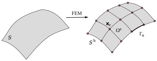
Figure 2. FE discretization of surface $S$.

5.1. Discretized Synthetical Kinematic Quantities

Within elements ${\Omega }^e$, the geometry is approximated by the nodal interpolations

$$\mathit{x} \approx {\mathit{x}}^{\mathrm{h}}={\displaystyle \sum }_{i=1}^n{\mathrm{N}}_i {\mathit{x}}_i,$$

(32)

where ${\mathrm{N}}_i={\mathrm{N}}_i\left({\mathsf{\xi }}^{\mathsf{\alpha }}\right)$ and $n$ denote the shape function and number of nodes, respectively. For shorthand notation, Equations (32) and (2) can be expressed as follows:

$$\mathit{x} \approx {\mathit{x}}^{\mathrm{h}}=N x_{\mathrm{e}} ,$$

(33)

$$a_{\mathsf{\alpha }}=N_{,{\mathsf{\xi }}^{\alpha }} x_{\mathrm{e}}$$

(34)

with $N_{,{\mathsf{\xi }}^{\alpha }}=\partial N/\partial {\mathsf{\xi }}^{\mathsf{\alpha }}$.

To write the discretized weak form of the governing equation, the variation of the tangent vector $a_{\mathsf{\alpha }}$, current nodal position vector of the nodes $\mathit{x}$, and the unit normal vector $n$ are required.

The variation of current position vector in Equation (33) and the tangent vector in Equation (34) is written as

$$\mathrm{\delta }\mathit{x}=N \mathrm{\delta }{x}_e$$

(35)

$$\mathrm{\delta }{a}_{\mathsf{\alpha }}=N_{,{\mathsf{\xi }}^{\alpha }} \mathrm{\delta }{x}_e$$

(36)

The variation of the unit normal vector is given by [30]

$$\mathrm{\delta }n=R_{\mathrm{A}}^{\mathsf{\alpha }} \mathrm{\delta }{a}_{\mathsf{\alpha }} ,$$

(37)

with

$$R_A^{\alpha }=-\left(a^{\alpha }\otimes n\right) .$$

(38)

The linearization of vector $n$ is followed from Equation (37) as

$$\Delta \mathrm{\delta }n=\left(-\Delta a^{\alpha }\otimes n\right) \mathrm{\delta }{a}_{\alpha }-\left(a^{\alpha }\otimes \Delta n\right) \delta a_{\alpha } ,$$

(39)

where Δa^α is can be found in [31]

$$\Delta a^{\alpha }=B^{\mathsf{\alpha }\mathsf{\beta }} \Delta a_{\mathsf{\beta }}$$

(40)

with $B^{\mathsf{\alpha }\mathsf{\beta }}={ \mathrm{a}}^{\mathsf{\alpha }\mathsf{\beta }} \left(n\otimes n\right)-a^{\mathsf{\beta }}\otimes a^{\mathsf{\alpha }}$, and $\Delta a_{\mathsf{\alpha }}$ is the same manner as $\mathrm{\delta }{a}_{\mathsf{\alpha }}$ from Equation (36). The variation of J is given respectively in [29]

$$\mathrm{\delta }\mathrm{J}=\mathrm{J} a^{\mathsf{\alpha }}· \mathrm{\delta }{a}_{\mathsf{\alpha }} .$$

(41)

Further, the variation and the linearization of ${\mathrm{a}}_{\mathsf{\alpha }\mathsf{\beta }}$ and ${\mathrm{a}}^{\mathsf{\alpha }\mathsf{\beta }}$ are:

$${\mathrm{\delta }\mathrm{a}}_{\mathsf{\alpha }\mathsf{\beta }}=a_{\mathsf{\alpha }} · \mathrm{\delta } a_{\mathsf{\beta }}+ \mathrm{\delta }{a}_{\mathsf{\alpha }} ·a_{\mathsf{\beta }} ,$$

(42)

$${\mathrm{\delta }\mathrm{a}}^{\mathsf{\alpha }\mathsf{\beta }}=a^{\mathsf{\alpha }} · \mathrm{\delta }{a}^{\mathsf{\beta }}+ \mathrm{\delta }{a}^{\mathsf{\alpha }} ·a^{\mathsf{\beta }} ,$$

(43)

$$\Delta {\mathrm{\delta }\mathrm{a}}_{\mathsf{\alpha }\mathsf{\beta }}=\Delta a_{\mathsf{\alpha }} · \mathrm{\delta } a_{\mathsf{\beta }}+ \mathrm{\delta }{a}_{\mathsf{\alpha }} · \Delta a_{\mathsf{\beta }} .$$

(44)

5.2. Discretized Weak Form of the Governing Equation

With the expressions in Section 5.1, the weak form is now discretized. Accordingly, Equation (20) can be written as follows:

$$\mathrm{\delta }{\mathrm{\Pi }}_{\mathrm{p}}\approx \mathrm{\delta }{\mathrm{\Pi }}_{\mathrm{p}}^{\mathrm{h}}= \mathrm{\delta }{x}^{\mathrm{T}} {\displaystyle \sum }_{\mathrm{e}=1}^{{\mathrm{n}}_{\mathrm{e}}}{f}_{\mathrm{p}}^{\mathrm{e}} ,$$

(45)

where

$$f_{\mathrm{p}}^{\mathrm{e}}:={{\displaystyle \int }}_{{\mathrm{\Omega }}_0^e}{g}_{\mathrm{p}}{ \mathrm{dA}}_{\mathrm{e}} .$$

(46)

In Equation (46), $g_{\mathrm{p}}$ is to be defined for a given type of cam.

The linearization can be expressed as

$$\Delta \mathrm{\delta }{\mathrm{\Pi }}_{\mathrm{p}}= \mathrm{\delta }{x}^{\mathrm{T}} k_{\mathrm{p}}\Delta x ,$$

(47)

where kp is the tangent matrix. It can be written as

$$k_{\mathrm{p}}={\displaystyle \sum }_{e=1}^{n_e}{k}_{\mathrm{p}}^{\mathrm{e}} .$$

(48)

5.3. Discretized Stabilization Terms

The weak form of the stabilization equation is discretized. The formula as shown in Equation (26) can be expressed as

$$\mathrm{\delta }{\mathrm{\Pi }}_{\mathrm{stab}}\approx \mathrm{\delta }{\mathrm{\Pi }}_{\mathrm{stab}}^{\mathrm{h}}= \mathrm{\delta }{x}^{\mathrm{T}} {\displaystyle \sum }_{\mathrm{e}=1}^{{\mathrm{n}}_{\mathrm{e}}}{f}_{\mathrm{stab}}^{\mathrm{e}} ,$$

(49)

where

$$f_{\mathrm{stab}}^{\mathrm{e}}:={{\displaystyle \int }}_{{\mathrm{\Omega }}_0^{\mathrm{e}}}{g}_{\mathrm{stab}}{ \mathrm{dA}}_{\mathrm{e}} .$$

(50)

The linearization of the stabilization functional can be expressed as

$$\Delta \mathrm{\delta }{\mathrm{\Pi }}_{\mathrm{stab}}= \mathrm{\delta }{x}^{\mathrm{T}} k_{\mathrm{stab}}\Delta x ,$$

(51)

where the tangent matrix can be written by

$$k_{\mathrm{stab}} :={\displaystyle \sum }_{\mathrm{e}=1}^{{\mathrm{n}}_{\mathrm{e}}}{k}_{\mathrm{stab}}^{\mathrm{e}} .$$

(52)

6. Finite Element Solution

6.1. Solution Procedure

The discretized weak form as shown in Equations (45) and (49) of the governing equation and the stabilization equation can be written as

$$\mathrm{\delta }{x}^{\mathrm{T}} \left[ f_{\mathrm{p}}+f_{\mathrm{stab}}\right]=0 \forall \mathrm{\delta }x ,$$

(53)

where

$$f_{\mathrm{p}} :={\displaystyle \sum }_{\mathrm{e}=1}^{{\mathrm{n}}_{\mathrm{e}}}{f}_{\mathrm{p}}^{\mathrm{e}} ;f_{\mathrm{stab}} :={\displaystyle \sum }_{\mathrm{e}=1}^{{\mathrm{n}}_{\mathrm{e}}}{f}_{\mathrm{stab}}^{\mathrm{e}} .$$

(54)

The nonlinear in Equation (53) can be solved by numerical methods. The Newton–Raphson method is used to solve this equation. Equation (53) can be described as

$$f\left(x\right):=f_{\mathrm{p}}+f_{\mathrm{stab}}=0 .$$

(55)

At iteration i, an approximation solution of cam profile can be sought and denoted by $x^{\mathrm{i}}$. The method can be described by Gouri Dhatt, et al. [32]

$$f\left(x^{\mathrm{i}}\right):=f\left(x^{\mathrm{i}-1}+\Delta x^{\mathrm{i}}\right)\approx 0,$$

(56)

The algorithm is obtained by developing this residual into a Taylor series in the vicinity of $x^{\mathrm{i}-1}$

$$f\left(x^{\mathrm{i}-1}+\Delta x^{\mathrm{i}}\right)=f\left(x^{\mathrm{i}-1}\right)+{\left[\frac{\partial f}{\partial x}\right]}_{x=x^{i-1}}\Delta x^{\mathrm{i}}+\dots =0 ,$$

(57)

and

$$x^i=x^{i-1}+\Delta x^i ,$$

(58)

By ignoring terms greater than one, we get

$$K \Delta x^i=-f\left(x^{i-1}\right),$$

(59)

where

$$K:=\frac{\partial f}{\partial x}=k_{\mathrm{p}}+k_{\mathrm{stab}}$$

(60)

is the tangent matrix.

6.2. Numerical Quadrature

For finite element computations, the integral for the weak form and the tangent matrices must be evaluated. These integrations can be performed on the element level. Since the integration is carried out in the finite element analysis of the reference configuration, the parameter domain coordinate ${\mathsf{\xi }}^{\mathsf{\alpha }}$∈ [−1, +1] must be transformed to this configuration (see Figure 3).

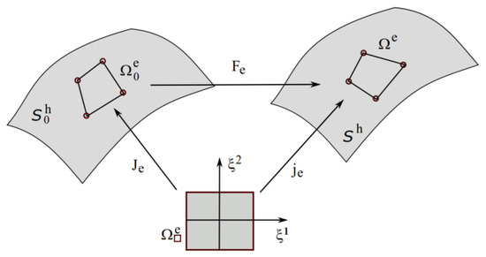
Figure 3. Mapping Gaussian integration between element ${\Omega }^{\mathrm{e}}$ of parameter domain P, element ${\Omega }_0^{\mathrm{e}}$ of discretized reference configuration ${\mathrm{S}}_0^{\mathrm{h}}$ and element ${\Omega }^{\mathrm{e}}$ of the discretized current configuration ${\mathrm{S}}^{\mathrm{h}}$.

The Jacobian can be calculated as follows [30]:

$$\begin{gathered} J_{\mathrm{e}}=\frac{\partial \mathit{X}}{\partial \mathsf{\xi }}\approx {\displaystyle \sum }_{\mathrm{A}}^{\mathrm{n}}{\mathit{X}}_{\mathrm{A}}\otimes \frac{\partial N_{\mathrm{A}}}{\partial \mathsf{\xi }} , \\ {j}_{\mathrm{e}}=\frac{\partial \mathit{x}}{\partial \mathsf{\xi }}\approx {\displaystyle \sum }_{\mathrm{A}}^{\mathrm{n}}{\mathit{x}}_{\mathrm{A}}\otimes \frac{\partial N_{\mathrm{A}}}{\partial \mathsf{\xi }} , \\ {F}_{\mathrm{e}}=j_{\mathrm{e}} J_{\mathrm{e}}^{-1} . \end{gathered}$$

(61)

The integration form is then carried out with the standard Gaussian quadrature on the parameter domain. Thus, from Equations (46) and (50), the governing equation of each element can be written as

$${{\displaystyle \int }}_{{\mathrm{\Omega }}_e}g{ \mathrm{dA}}_{\mathrm{e}}={{\displaystyle \int }}_{{\mathrm{\Omega }}_e}{g}_p{\mathrm{dA}}_{\mathrm{e}}+{{\displaystyle \int }}_{{\mathrm{\Omega }}_e}{g}_{\mathrm{stab}}{\mathrm{dA}}_{\mathrm{e}}$$

(62)

The integration in Equation (62) is computed by

$$\begin{array}{cc}\hfill {{\displaystyle \int }}_{{\mathrm{\Omega }}_e}g {\mathrm{dA}}_{\mathrm{e}}& :={{\displaystyle \int }}_{\mathrm{\Omega }}{g}_{\mathrm{p}}\left(\mathsf{\xi }\right)\det J_{\mathrm{e}}\mathrm{d}+{{\displaystyle \int }}_{\mathrm{\Omega }}{g}_{\mathrm{stab}}\left(\mathsf{\xi }\right)\det J_{\mathrm{e}}\mathrm{d}\hfill \\ \hfill & ={{\displaystyle \int }}_{-1}^{+1}{{\displaystyle \int }}_{-1}^{+1}{g}_p\left({\mathsf{\xi }}^{\alpha }\right)\det J_{\mathrm{e}} \mathrm{d}{\mathsf{\xi }}^1\mathrm{d}{\mathsf{\xi }}^2+{{\displaystyle \int }}_{-1}^{+1}{{\displaystyle \int }}_{-1}^{+1}{g}_{\mathrm{stab}}\left({\mathsf{\xi }}^{\alpha }\right)\det J_{\mathrm{e}} \mathrm{d}{\mathsf{\xi }}^1\mathrm{d}{\mathsf{\xi }}^2.\hfill \end{array}$$

(63)

The integration will be done numerically. ${\mathrm{n}}_{\mathrm{gp}}$ is representative for the number of Gauss points. Hence, the integral in Equation (63) will be approximated by

$${{\displaystyle \int }}_{{\mathrm{\Omega }}_e}g{ \mathrm{dA}}_{\mathrm{e}}\approx {\displaystyle \sum }_{\mathrm{gp}=1}^{{\mathrm{n}}_{\mathrm{gp}}}{g}_{\mathrm{p}}\left({\mathsf{\xi }}_{\mathrm{gp}}\right)\det J_{\mathrm{e}}{\mathrm{W}}_{\mathrm{p}}+{\displaystyle \sum }_{\mathrm{gp}=1}^{{\mathrm{n}}_{\mathrm{gp}}}{g}_{\mathrm{stab}}\left({\mathsf{\xi }}^{\mathsf{\alpha }}\right)\det J_{\mathrm{e}}{\mathrm{W}}_{\mathrm{p}}.$$

(64)

Here, ${\mathrm{W}}_{\mathrm{p}}$ is weighting factors and ${\mathsf{\xi }}_{\mathrm{gp}}$ denotes the coordinates of the evaluation points. The integration for the whole system can be computed as follows:

$${\displaystyle \sum }_{\mathrm{e}=1}^{{\mathrm{n}}_{\mathrm{e}}}{{\displaystyle \int }}_{{\mathrm{\Omega }}_{\mathrm{e}}}{\mathrm{g} \mathrm{dA}}_{\mathrm{e}}\approx {\displaystyle \sum }_{\mathrm{e}=1}^{{\mathrm{n}}_{\mathrm{e}}}{\displaystyle \sum }_{\mathrm{gp}=1}^{{\mathrm{n}}_{\mathrm{gp}}}{g}_{\mathrm{p}}\left({\mathsf{\xi }}_{\mathrm{gp}}\right)\det J_{\mathrm{e}}{\mathrm{W}}_{\mathrm{p}}+{\displaystyle \sum }_{\mathrm{e}=1}^{{\mathrm{n}}_{\mathrm{e}}}{\displaystyle \sum }_{\mathrm{gp}=1}^{{\mathrm{n}}_{\mathrm{gp}}}{g}_{\mathrm{stab}}\left({\mathsf{\xi }}^{\mathsf{\alpha }}\right)\det J_{\mathrm{e}}{\mathrm{W}}_{\mathrm{p}} .$$

(65)

6.3. Computational Algorithm

This section presents a computational to solve a cam profile. With the above-discussed framework, the computational algorithm of a cam profile that satisfies a prescribed displacement of the follower is given in Table 1.

Table 1. The computational algorithm.

1. Defined the initial configuration

2. Step loop

Given parameters: tolerances for the reduced penalty parameter $\mu$, and augmentedLagrangian; penalty parameter $\mathrm{ϵ}$; parameter $\mathsf{\lambda }$

2.1. Newton iteration:

Compute $k_{\mathrm{p}},k_{\mathrm{stab}}, f_{\mathrm{p}}$, $f_{\mathrm{stab}}$, as shown in Equations (48), (52), and (54) respectively Apply boundary conditions Step 1: Load step for penalty method Step 2: Reduce parameter $\mu$ Step 3: Update new parameter $\mathsf{\lambda }$ of Augmented Lagrangian method following as equation ${\mathsf{\lambda }}_{\mathrm{new}}=\mathrm{ϵ} \mathrm{g}+{ \mathsf{\lambda }}_{\mathrm{old}}$ Solve $K \Delta x^{\mathrm{i}}=-f\left(x^{\mathrm{i}-1}\right)$ and update $x^{\mathrm{i}}=x^{\mathrm{i}-1}+\Delta x^{\mathrm{i}}$

Update reference configuration

7. Case Study

This section presents a case study to demonstrate the procedure of this work. We consider the cam mechanism with a flat-face follower for illustration. The finite element is therefore reduced to line elements. With the general designing framework discussed above, an explicit expression for the follower displacement is required. The expression is, however, generally dependent on the type of cam. The cam curves resulted from the proposed framework are compared with the analytical solution.

7.1. Computation of Cam Flat-Face Follower

With the flat-face follower, as shown in Figure 4, the function of the follower displacement ${\mathrm{s}}_0$ can be written as follows:

$${\mathrm{s}}_0=\mathrm{f}\left(\mathsf{\phi }\right) ,$$

(66)

where $\mathsf{\phi }$ is the angle of the camshaft, and the displacement function $\mathrm{f}\left(\mathsf{\phi }\right)$ is shown in Appendix A.

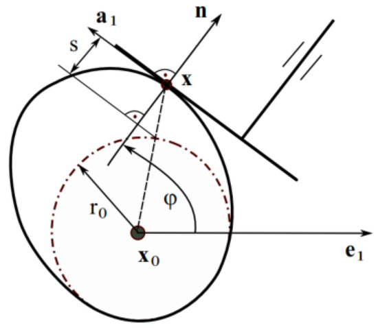
Figure 4. Calculation parameters of cam flat-face follower.

For cam plate, we can describe the tangent vector and others with $\mathsf{\alpha }$ = 1 and $\mathsf{\beta }$ = 1. ${\mathsf{\xi }}^1$ is denoted by ξ. From the variation of the stabilized equation (see Equation (26)), $f_{\mathrm{stab}}^{\mathrm{e}}$ can be computed as follows:

$$f_{\mathrm{stab}}^{\mathrm{e}}={{\displaystyle \int }}_{{\mathrm{\Omega }}_0^{\mathrm{e}}}\mathsf{\mu }\left({\mathrm{A}}^{11}-{ \mathrm{a}}^{11}\right) N_{,\mathsf{\xi }}^{\mathrm{T}} a_1{ \mathrm{dA}}_{\mathrm{e}} .$$

(67)

Likewise, the tangent matrix is calculated by

$$k_{\mathrm{stab}}^{\mathrm{e}}=\left(k_{\mathrm{stab}1}^{\mathrm{e}}+k_{\mathrm{stab}2}^{\mathrm{e}}\right) ,$$

(68)

where

$$\begin{gathered} k_{\mathrm{stab}1}^{\mathrm{e}}={{\displaystyle \int }}_{{\mathrm{\Omega }}_0^e}2{\mathsf{\mu } \mathrm{a}}^{11} N_{,}^{\mathrm{T}} a_1\otimes a_1{N}_{,\mathsf{\xi }}^T{ \mathrm{dA}}_{\mathrm{e}} , \\ {k}_{\mathrm{stab}2}^{\mathrm{e}}={{\displaystyle \int }}_{{\mathsf{\Omega }}_0^e}\mathsf{\mu }\left({\mathrm{A}}^{11}-{ \mathrm{a}}^{11}\right) N_{,\mathsf{\xi }}^T N_{,\mathsf{\xi }}{ \mathrm{dA}}_{\mathrm{e}} . \end{gathered}$$

(69)

As shown in Figure 4, the displacement of the follower can be computed as

$$\mathrm{s}:= \mathit{x}·n-{ \mathrm{r}}_0 .$$

(70)

Taking the variation of the current displacement in Equation (70) is presented by

$$\mathrm{\delta }\mathrm{s}= \mathrm{\delta }\mathit{x} ·n+\mathit{x} · \mathrm{\delta }n .$$

(71)

The angle of the camshaft can be written as (see Figure 4)

$$\mathsf{\phi }=\arccos \left(n ·e_1\right).$$

(72)

The variation of ${\mathrm{s}}_0$ can be also computed by

$${\mathrm{\delta }\mathrm{s}}_0=-{\mathrm{d}}_{\mathrm{c}} e_1· \mathrm{\delta }n .$$

(73)

In Equation (73), ${\mathrm{d}}_{\mathrm{c}}$ is calculated in Appendix A.

From the calculation above, $f_p^e$ can be simply obtained by

$$f_p^e={{\displaystyle \int }}_{{\mathrm{\Omega }}_0^e}\left(N^{T}n+N_{,\mathsf{\xi }}^T R_{\mathrm{A}}^T b\right){ \mathrm{dA}}_{\mathrm{e}} ,$$

(74)

where, $R_{\mathrm{A}}:= R_{\mathrm{A}}^1$. The tangent matrix is

$$k_p^e=k_{p1}^e+k_{p2}^e.$$

(75)

Here

$$\begin{gathered} k_{p1}^e={{\displaystyle \int }}_{{\mathrm{\Omega }}_0^e}\mathrm{ϵ}\left(n\otimes n N+n\otimes b R_{\mathrm{A}} N_{,\mathsf{\xi }}\right){ \mathrm{dA}}_{\mathrm{e}} \\ +{{\displaystyle \int }}_{{\mathrm{\Omega }}_0^e}\mathrm{ϵ} N_{,\mathsf{\xi }}^T R_A^T\left(b\otimes n N+b\otimes b R_{\mathrm{A}} N_{,\mathsf{\xi }}\right){ \mathrm{dA}}_{\mathrm{e}} , \end{gathered}$$

(76)

and

$$k_{p2}^e={{\displaystyle \int }}_{{\mathrm{\Omega }}_0^e}\left(N^T{R}_A N_{,\mathsf{\xi }}+N_{,\mathsf{\xi }}^T R_A^T G_1-N_{,\mathsf{\xi }}^T G_2 N_{,\mathsf{\xi }}\right){ \mathrm{dA}}_{\mathrm{e}} .$$

(77)

Tensor $b$ in Equation (76) and tensors $G_1$, $G_2$ in Equation (77) are defined in Appendix A.

In the example, the cycloid function for the displacement of the follower as shown in Equations (A1) and (A2) in Appendix A is used for the design of the cam profile. The types of motion programs are rise, fall, and dwell. These motions are defined by the angle of segments, i.e., ${\beta }_1={\beta }_2={\beta }_3={120}^{°}$ and the lift L = 5 mm. By using the computational algorithm in Section 6.3, the cam profile is shown in Figure 5a and the kinematic characteristics of the follower including displacement, velocity, and acceleration are presented in Figure 5b–d. The finite element solution of the cam profile is compared with the analytical solution as shown in Figure 5. From this figure, it can be seen that there are very small differences between the FE solution and the analysis solution.

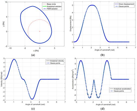
Figure 5. Compare between FE solution with 128 elements and analytical solution (a) comparison of cam profile; (b) comparison of displacement; (c) comparison of velocity; (d) comparison of acceleration.

In this example, 128 elements are used to compute the cam profile. In the penalty step, the maximum difference between the FE displacement and the input displacement is small, i.e., ε = 1.9 × 10⁻³. For the second step, the stabilization parameter µ is reduced from 100 to 25, which increases the accuracy in the displacement to ε = 7.0282 × 10⁻⁵. For the augmented step, the accuracy is further improved with ε = 2.6133 × 10⁻⁵.

Next, the size of the cam is considered in the cam design process since it decides the cost of the cam follower. The cam size is influenced by the base circle ${\mathrm{r}}_{\mathrm{O}}$. Usually, a minimum base circle, denoted by ${\mathrm{r}}_{{\mathrm{O}}_{\min }}$, can be defined by (see Robert L. Norton [23])

$${\mathrm{r}}_{{\mathrm{O}}_{\min }}>{\mathsf{\rho }}_{\min }-{\mathrm{s}}_{{@}_{\mathrm{amin}}}-{\mathrm{a}}_{\min } ,$$

(78)

where ${\mathsf{\rho }}_{\min }$, ${\mathrm{a}}_{\min }$, ${\mathrm{s}}_{{@}_{\mathrm{amin}}}$ are the minimum radius of curvature, minimum acceleration, and the displacement value at ${\mathrm{a}}_{\min }$, respectively.

In order to determine the minimum base circle, the parameters including ${\mathsf{\rho }}_{\min }$, ${\mathrm{s}}_{{@}_{\mathrm{amin}}}$, and ${\mathrm{a}}_{\min }$ need to be computed. The minimum radius of curvature ${\mathsf{\rho }}_{\min }$ is calculated from Equation (7). Values of ${\mathrm{s}}_{{@}_{\mathrm{amin}}}$ and ${\mathrm{a}}_{\min }$ are determined from the displacement and acceleration functions. Substituting values of the parameters into Equation (78), the minimum base circle is 3.9878 mm. In addition, with the cam flat-face follower, the radius of curvature must be positive to maintain the contact between the cam and the follower.

7.2. Influence of Parameters $\mathrm{ϵ}$ and µ

Next, the influence of penalty parameters $\mathrm{ϵ}$ and µ is discussed in this section. The accuracy of the cam profile is estimated by parameter $\mathrm{ϵ}$ as shown in Figure 6a. It is clearly seen that an accurate solution is obtained for a sufficiently large $\mathrm{ϵ}$. However, it should be noted that for the augmented method, a much smaller penalty parameter is already sufficient for the comparative accuracy due to the extra correction loop.

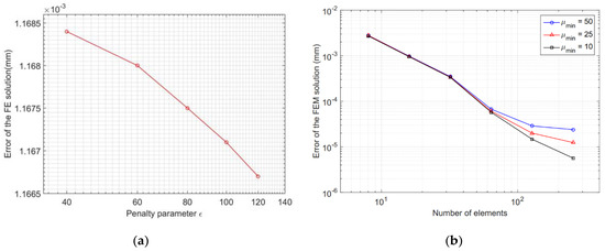
Figure 6. Influence of parameters $\mathrm{ϵ}$ and µ: (a) penalty parameter $\mathrm{ϵ}$; (b) parameter µ.

Figure 6b further shows the convergence of the finite element calculation with mesh refinement for three minimum values of the parameter µ = 50, 25, and 10. It is observed from the figure that the rate of convergence increases with decreasing the parameter µ. On the other hand, for the fine meshes, parameter µ affects the convergent rate significantly, i.e., the smaller stabilization parameter, the more accuracy is obtained.

8. Conclusions

This paper presents a new and general computational formulation for the synthesis of cam mechanisms using the finite element method. The formulation is based on a general theoretical description of the cam curve in curvilinear coordinates. The governing equation for the synthesis of cam profile is proposed. The penalty-type functional is proposed for the weak form. The stabilization functional is further added for convexity of the total potential. The discretization of the weak form is derived in the framework of the finite element. The Gaussian quadrature is used to integrate the finite element computation. The cam profile is obtained by solving a nonlinear system of equations resulting from minimizing the total functional.

The case study of the flat-face cam mechanism demonstrates that the formulation is able to handle all aspects accurately, robustly, and efficiently. The proposed framework can be applied for more general cam mechanisms, which is a subject of future work.

References

- Uicker, J.J.; Pennock, G.R.; Shigley, J.E.; McCarthy, J.M. Theory of Machines and Mechanisms, 5th ed.; Oxford University Press: New York, NY, USA, 2003. [Google Scholar]
- Mermelstein, S.P.; Acar, M. Optimising cam motion using piecewise polynomials. Eng. Comput. 2003, 19, 241–254. [Google Scholar] [CrossRef][Green Version]
- Cardona, S.; Zayas, E.; Jordi, L.; Català, P. Synthesis of displacement functions by Bézier curves in constant-breadth cams with parallel flat-faced double translating and oscillating followers. Mech. Mach. Theory 2013, 62, 51–62. [Google Scholar] [CrossRef]
- Sateesh, N.; Rao, C.S.; Reddy, T.A.J. Optimisation of cam-follower motion using B-splines. Int. J. Comput. Integr. Manuf. 2009, 22, 515–523. [Google Scholar] [CrossRef]
- Jiang, J.K.; Iwai, Y.R. Improving the B-Spline Method of Dynamically-Compensated Cam Design by Minimizing or Restricting Vibrations in High-Speed Cam-Follower Systems. J. Mech. Des. 2009, 131, 041003. [Google Scholar] [CrossRef]
- Nguyen, T.T.N.; Nguyen, V.S.; Nguyen, T.B.N.; Vu, T.L. An Evaluation of B-Spline for Synthesis of Cam Motion with a Large Number of Output Conditions. In Advances in Engineering Research and Application, Proceedings of the International Conference on Engineering Research and Applications, ICERA 2020, Thai Nguyen, Vietnam, 1–2 December 2020; Nguyen, D.C., Vu, N.P., Long, B.T., Puta, H., Eds.; Springer: Heidelberg, Germany.
- Müller, M.; Hüsing, M.; Beckermann, A.; Corves, B. Linkage and Cam Design with MechDev Based on Non-Uniform Rational B-Splines. Machines 2020, 8, 5. [Google Scholar] [CrossRef]
- Nguyen, T.T.N.; Kurtenbach, S.; Hüsing, M.; Corves, B. A general framework for motion design of the follower in cam mechanisms by using non-uniform rational B-spline. Mech. Mach. Theory 2019, 137, 374–385. [Google Scholar] [CrossRef]
- Nguyen, T.T.N.; Kurtenbach, S.; Hüsing, M.; Corves, B. Evaluating the Knot Vector to Synthesize the Cam Motion Using NURBS. Mech. Mach. Sci. 2018, 50, 209–216. [Google Scholar] [CrossRef]
- Nguyen, T.T.N.; Kurtenbach, S.; Hüsing, M.; Corves, B. Improving the Kinematics of Motion Curves for Cam Mechanisms Using NURBS. Mech. Mach. Sci. 2018, 52, 79–88. [Google Scholar] [CrossRef]
- Ouyang, T.; Wang, P.; Huang, H.; Zhang, N.; Chen, N. Mathematical modeling and optimization of cam mechanism in delivery system of an offset press. Mech. Mach. Theory 2017, 110, 100–114. [Google Scholar] [CrossRef]
- Qin, W.; Chen, Y. Study on optimal kinematic synthesis of cam profiles for engine valve trains. Appl. Math. Model. 2014, 38, 4345–4353. [Google Scholar] [CrossRef]
- Xia, B.-Z.; Liu, X.-C.; Shang, X.; Ren, S.-Y. Improving cam profile design optimization based on classical splines and dynamic model. J. Cent. South. Univ. 2017, 24, 1817–1825. [Google Scholar] [CrossRef]
- Yu, J.; Huang, K.; Luo, H.; Wu, Y.; Long, X. Manipulate optimal high-order motion parameters to construct high-speed cam curve with optimized dynamic performance. Appl. Math. Comput. 2020, 371, 124953. [Google Scholar] [CrossRef]
- Flores, P. A Computational Approach for Cam Size Optimization of Disc Cam-Follower Mechanisms with Translating Roller Followers. J. Mech. Robot. 2013, 5, 041010. [Google Scholar] [CrossRef]
- Navarro, O.; Wu, C.-J.; Angeles, J. The size-minimization of planar cam mechanisms. Mech. Mach. Theory 2001, 36, 371–386. [Google Scholar] [CrossRef]
- Yu, Q.; Lee, H.P. Size optimization of cam mechanisms with translating roller followers. Proc. Inst. Mech. Eng. Part C 1998, 212, 381–386. [Google Scholar] [CrossRef]
- Rothbart, H.A. Cam Design Handbook; McGraw-Hill: New York, NY, USA, 2004. [Google Scholar]
- Myszka, D.H. Machines and Mechanicsms: Applied Kinematic Analysis, 4th ed.; Pren-tice Hall: Upper Saddle River, NJ, USA, 2012. [Google Scholar]
- Gupta, B.V.R. Theory of Machines: Kinematics and Dynamics; I.K. international Pvt: New Delhi, India, 2010. [Google Scholar]
- Li, F.; Feng, X. The design of parallel combination for cam mechanism. Procedia Environ. Sci. 2011, 10, 1343–1349. [Google Scholar]
- Shala, A.; Likaj, R. Analytical Method for Synthesis of Cam Mechanism. Int. J. Curr. Eng. Technol. 2013, 133. [Google Scholar]
- Norton, R. Design of Machinery; McGraw-Hill: New York, NY, USA, 2003. [Google Scholar]
- Wu, L.-I.; Chang, W.-T.; Liu, C.-H. The design of varying-velocity translating cam mechanisms. Mech. Mach. Theory 2007, 42, 352–364. [Google Scholar] [CrossRef]
- Chen, F.Y. Mechanics and Design of Cam Mechanisms; Pergamon Press: New York, NY, USA, 1982. [Google Scholar]
- Biswas, A.; Stevens, M.; Kinzel, G.L. A comparison of approximate methods for the analytical determination of profiles for disk cams with roller followers. Mech. Mach. Theory 2004, 39, 645–656. [Google Scholar] [CrossRef]
- Hsieh, J.-F. Design and analysis of cams with three circular-arc profiles. Mech. Mach. Theory 2010, 45, 955–965. [Google Scholar] [CrossRef]
- Hsieh, J.-F. Design and analysis of indexing cam mechanism with parallel axes. Mech. Mach. Theory 2014, 81, 155–165. [Google Scholar] [CrossRef]
- Sauer, R.A.; Duong, T.X.; Corbett, C.J. A computational formulation for constrained solid and liquid membranes considering isogeometric finite elements. Comput. Methods Appl. Mech. Eng. 2014, 271, 48–68. [Google Scholar] [CrossRef]
- Swinggers, P. Computational Contact Mechanics, 2nd ed.; Springer: Heidelberg, Germany, 2006. [Google Scholar]
- Sauer, R.A. A contact theory for surface tension driven systems. Math. Mech. Solids 2016, 21, 305–325. [Google Scholar] [CrossRef]
- Dhatt, G.; Touzot, G.; Lefrançois, E. Finite Element Method, 1st ed.; Wiley-ISTE: Hoboken, NJ, USA, 2012. [Google Scholar]
Publisher’s Note: MDPI stays neutral with regard to jurisdictional claims in published maps and institutional affiliations. |
© 2021 by the authors. Licensee MDPI, Basel, Switzerland. This article is an open access article distributed under the terms and conditions of the Creative Commons Attribution (CC BY) license (https://creativecommons.org/licenses/by/4.0/).