Abstract
A comprehensive multiparameter model is proposed for underwater wireless optical communication (UWOC) channels to integrate the effects of absorption, scattering, and dynamic turbulence. The simulation accuracy is further improved by the combined use of the subharmonic method and the strict sampling constraint method by comparing the phase structure function with the theoretical value. The average light intensity and scintillation index are analyzed using the channel parameters of absorption, scattering, turbulence, flow velocity, and transmission distance. Under weak or medium turbulence, the bit error rate (BER) performance can be effectively improved by increasing the transmitting light power. The power penalty of a 50 m UWOC channel is 5.8 dBm from pure seawater to ocean water and 1.0 dBm from weak turbulence to medium turbulence, with the BER threshold of 10−6.
1. Introduction
Underwater wireless optical communication (UWOC) technology has attracted much attention because of its high transmission data rate, low link delay, high communication security, and low implementation costs [1,2,3]. In recent years, experimental UWOC systems have achieved data rates of Gbps and distances of tens of meters based on laser sources and advanced modulation formats [4,5,6,7,8,9,10]. However, several challenges remain regarding UWOC. The optical signal suffers from severe attenuation and multipath fading caused by absorption and scattering effects even though the transmission wavelength has been selected within the blue and green spectrum window [11]. Moreover, the optical signal is less tolerant to water turbulence than the traditional radio-frequency signal [12], which limits the communication performance in real seawater environments.
Several models have been developed to analyze the optical characteristics of the UWOC channel. The Beer-Lambert law is the most widely used theoretical basis by which to model the absorption and scattering effects as exponential attenuation [1]. To take into account the extra influence of scattered light on the total received light, the radiative transfer equation (RTE) is employed to generate the beam spread function [13]. However, it is difficult to determine an exact analytical solution for the RTE; only approximate solutions can be derived, and temporal distribution information is lost in this process. In contrast to analytical solutions for the RTE, numerical solutions have been proved to provide a more complete description of a light beam along the channel [14]. The optical path loss due to absorption and scattering effects in different water types has been calculated by a numerical RTE solution [15]. The Henyey-Greenstein scattering phase function has been applied in the RTE to analyze the spatial spreading and temporal broadening characteristics of the light beam with the change of seawater attenuation coefficients [16].
The above models can only analyze absorption and scattering effects in the steady water link. Besides, the turbulence-induced-scintillation of the optical signal is a common issue during underwater light transmission. Turbulence, which is caused by random variations in pressure, temperature, and salinity, is characterized as refractive index fluctuations and can severely distort the propagating light and considerably degrade the bit error rate (BER) performance of a UWOC system. However, the impact of the underwater turbulence has been ignored in many previous studies [1]. In recent years, the Kolmogorov spectrum model has been applied to analyze the underwater optical turbulence via Monte Carlo phase screens [17], a model similar to that used in free-space optical communications.
Since absorption, scattering, and turbulence coexist in seawater, a comprehensive model that includes all these effects should be established to describe the underwater optical transmission. Recently, J. Zhang [18] developed Monte Carlo phase screens from the wave method to ray method through the generalized Snell’s law, so that the RTE can be merged into the phase screen model. In this case, RTE is generated to describe absorption and scattering and phase screens are generated to describe turbulence. In this paper, we propose a novel comprehensive multiparameter model for the UWOC system to simulate the effects of absorption, scattering, and dynamic turbulence, simultaneously. We utilize both the subharmonic method and the strict sampling constraint method to enhance the modeling accuracy. Based on the model, the spatial and temporal effects of absorption, scattering, and turbulence on the transmission light are compared, and the BER performance of the UWOC system is analyzed.
2. Comprehensive Multiparameter Model for UWOC Channels
The underwater optical channel is affected by absorption, scattering, and turbulence. The random effect of the turbulence is related to the light position, whereas absorption and scattering uniformly affect the whole light beam. Meanwhile, the laser transmission process can be considered by the split-step beam propagation method [19] as alternate steps of partial propagation in the isotropic material, and interactions with the material with the inhomogeneous refractive index n(x, y, z). In this way, the absorption and scattering effects, as well as the turbulence effect, can be both considered in such alternate steps.
Figure 1 shows the schematic description of the channel model. The transmission process can be separated into refraction parts and diffraction parts [20]. The turbulence effect is treated as thin phase screens that only change the light propagation directions [21]. Then, all the light keep their own directions until reaching the next phase screen, with the light intensity attenuating due to absorption and scattering effects along the path. In the end, a Fresnel diffractive lens is set to converge the spatial light to the receiver.
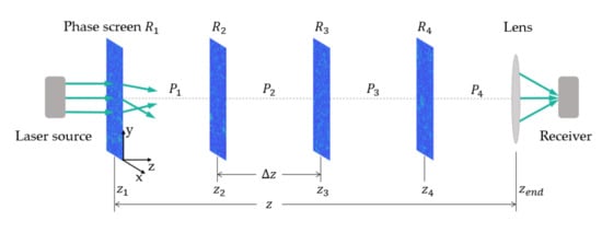
Figure 1.
Schematic description of the beam propagation model of the UWOC channel.
The collimated laser source is modeled by a Gaussian beam as . The optical field on the screen plane is and the optical field on the screen plane can be expressed as:
where and are spatial coordinates on the screens and is the distance of each propagation segment. is the refraction operator. The phase can be obtained from the underwater turbulence refractive index power spectrum density (PSD). is the diffraction operator, where is the spatial frequency of the optical field on the screen. Fourier transforms and a transfer function are used here to describe the Fresnel diffraction process.
Regarding the refraction part, the phase values on a screen can be written as:
where and are the discrete spatial frequencies in x and y directions, respectively. The Fourier coefficients obey the complex Gaussian distribution with zero mean and the variance given by [22]:
where and are the sizes of the screen, and is the underwater turbulence refractive index PSD as [23]:
where , is the optical wavenumber, is the dissipation rate of turbulent kinetic energy per unit mass of fluid ranging from to , is the dissipation rate of mean-squared temperature ranging from to , defines the ratio of the temperature contribution to the salinity contribution to the refractive index spectrum, ranging from −5 to 0, and is the Kolmogorov microscale length. The constants are = 1.863 × 10⁻², = 1.9 × 10⁻⁴, and = 9.41 × 10⁻³. In real underwater environments, the refractive index of water will slightly increase as the pressure increases or the temperature decreases within the normal range [24], and the dissipation rate of mean-squared temperature in the PSD function in Equation (4) is related to the temperature gradient of water [23].
In this way, the phase values on the screen can be obtained to model the effect of underwater turbulence. In addition to spatial randomness of static turbulence, the model is extended to dynamic scenarios based on the Taylor frozen-turbulence hypothesis [25], which treats temporal variations of the turbulence at a location as its advection by the turbulence flow. Here, we also introduce the long-size phase screens and the parameter of water flow velocity to simulate the temporal properties of the channel.
Regarding the diffraction part, the absorption and scattering effects can be concisely described as the exponential light attenuation as [26]:
where is the initial light intensity, z is the transmission distance, and are the absorption coefficient and the scattering coefficient of seawater, respectively. The coefficients and will vary with different water types, climatic conditions, and optical wavelengths [1]. The light transmission path in each propagation segment (typically on the scale of meter) is much longer than the light position movement on the transverse plane (typically on the scale of millimeter). Therefore, it is reasonable to neglect the distance difference among each light path and unify the transmission distance of the whole light beam as . Since the light intensity satisfies , the optical field after passing through a distance of seawater should be:
where represents the optical field after passing through the same distance of vacuum. Moreover, we develop the known transfer function for vacuum [27] to the transfer function for seawater transmission as:
thereby integrating underwater absorption and scattering effects into the diffraction parts of the model.
Based on the above channel model, the comprehensive analysis of all the relevant parameters’ effects on the UWOC channel can be carried out, including the absorption and scattering coefficients , the turbulence inherent properties , the macroscopic velocity of water flow , and the total transmission distance . In view of the complexity of the transmission process and the multitude of parameters, a qualitative evaluation of the static received spots is first conducted at the lens position. The results can also visually prove the availability of our model. Then, the quantitative analysis of the dynamic underwater channel is completed by studying the probability density distribution function (PDF) of the received light intensity in succession.
Furthermore, the UWOC performance is evaluated through the PDF data. The BER of the on–off keying modulation system can be calculated by the Gauss error function as:
where the parameter ζ is the square root of the signal-to-noise ratio (SNR) as:
where represents the average received light intensity and is its variance. Both can be obtained from the PDFs through numerical simulations. is the additive white Gaussian noise (AWGN) introduced by the communication system.
3. Optimization of the Phase Screen Model
Modeling errors will be induced into the phase screens because of the numerical sampling. We propose using the subharmonic method [28] and the strict sampling constraint method to compensate for the insufficient discrete sampling.
First, the sampling points of low spatial frequencies are increased by adding a subharmonic phase screen to the original screen. A subharmonic phase screen is a sum of -layers of screens given by:
where each value of corresponds to a different 3 × 3 grid of frequency, and the frequency grid spacing is .
Moreover, the geometry (taking the y–z plane for example) of the diffraction process is illustrated in Figure 2, where and denote the interested observation region on the screens, and α is the deviation angle of the propagation beam; the maximum angle is reckoned as:
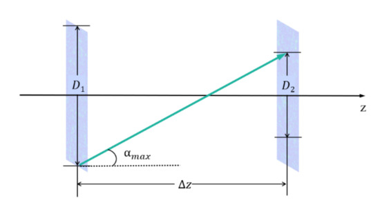
Figure 2.
Schematic diagram of the geometric relationship in the diffraction process.
According to the Nyquist sampling theorem, the grid spacing of the numerical simulation model should be constrained as , where is the maximum spatial frequency of interest and satisfies . Therefore, the upper bound of the grid spacing can be derived as:
According to Equation (12), strict constraint on can be applied to improve the accuracy of the model since the larger the observation region (), the more complete the information. The joint application of the subharmonic method and the strict sampling constraint method provides flexibility for the model optimization, consistent with the analytical theory.
The phase structure function (PSF) is employed as a statistical reference to verify the accuracy of the established phase screen model. The theoretical expression of the underwater turbulence PSF is [29]:
where is the separation distance between two points on the phase front. Meanwhile, PSF generated from the existing phase screens is defined as [30]:
where represents the coordinate on a phase screen. A statistical average of 1000 temporal-coherent phase screens is carried out and then compared with the theoretical PSF. The channel parameters are set as follows: , , , , , , , and .
We also define the matching degree between the model and theory by normalized 2-norm as:
where is the initial PSF of the model without optimization and is each PSF obtained by adjusting the optimization conditions. The range of is (); the closer the value is to 1, the better the matching degree.
Figure 3 shows the optimization performance of the subharmonic method. The PSF curve becomes closer to the dotted line representing the theoretical value, with the subharmonic layer number increasing from 0 to 5. However, at , the low-frequency sampling is overcompensated, resulting in the deviation from the theoretical curve again. The PSF matching degrees with 0, 3, 5, and 6 are 0, 1.07%, 48.09%, and −34.68%, respectively. Accordingly, when the subharmonic method is applied alone, a maximum matching degree of 48.09% can be realized with set to 5. The optimization performance is limited because the number of the subharmonic layers can only change in the integer range.
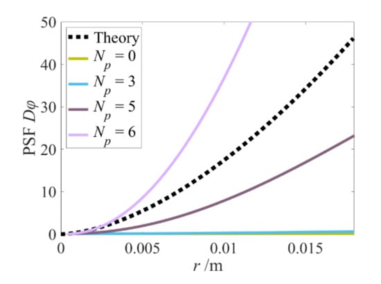
Figure 3.
The average PSF of the simulation model with subharmonic phase screens.
The modeling accuracy can be further improved by adjusting the value of the grid spacing. Figure 4 shows the optimization performance when both the subharmonic method and the strict sampling constraint method are utilized, with . The PSF curve becomes closer to the theoretical value as the grid spacing decreases. The PSF matching degrees with m, m, m, and m are 1.85%, 9.52%, 48.09%, and 96.19%, respectively. Finally, the phase screen model is effectively optimized by the joint application of the two methods, and is verified to achieve the matching degree of 96.19% with the theoretical statistics. However, it should be noted that the decrease of generally means an increase of Monte Carlo simulation workload; thus, it is important to make a trade-off between modeling accuracy and efficiency.
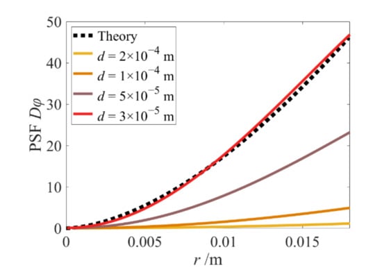
Figure 4.
The average PSF of the simulation model with different sampling spacing.
4. Simulation and Discussion
The UWOC performance will be simulated based on the established comprehensive model. Table 1 shows the values of the related parameters.

Table 1.
Parameter values in the simulation.
4.1. Received Light Spots
Figure 5 shows the spatial intensity distributions of the received spots after an 80 m distance underwater transmission. Four cases are considered: in the vacuum (see Figure 5a), in the water with turbulence only (see Figure 5b), in the water with attenuation only (see Figure 5c), and in the water with turbulence and attenuation simultaneously (see Figure 5d). The turbulence properties in Figure 5b, d are set as follows: , , and . The absorption and scattering coefficients in Figure 5c,d are and . A comparison of the results in Figure 5a,b shows that the turbulence effect results primarily in the beam diffusion and uneven spatial distribution of light intensity, which subsequently deteriorates the communication performance. In Figure 5a,c, the absorption and scattering effects cause uniform attenuation of light intensity. Considering the receiving intensity threshold, the attenuation in ocean water may bring more challenges to signal receiving in a UWOC system.
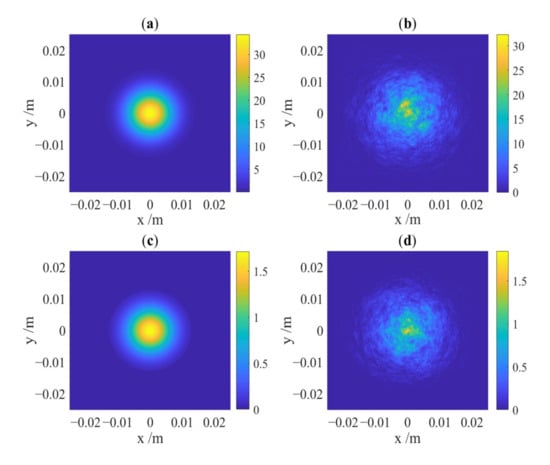
Figure 5.
Intensity distributions of the received spots in (a) the vacuum, (b) the water with turbulence only, (c) the water with attenuation only, and (d) the water with attenuation and turbulence simultaneously.
Figure 6 shows the spatial intensity distributions of the received spots after passing through different turbulence channels. The parameters in Figure 6a are as follows: , , and . The parameters are changed to in Figure 6b, in Figure 6c, and in Figure 6d. The decrease of , which means the slower consumption of the turbulence kinetic energy, the increase of , which means the larger temperature gradient of water, and the approach of to 0, which means more contributions from salinity than temperature, all imply the aggravation of the turbulence effect in a UWOC system.
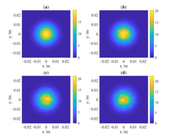
Figure 6.
Intensity distributions with turbulence properties of (a) , , ; (b) , , ; (c) , , ; (d) , , .
4.2. PDF of the UWOC Channel
In dynamic scenarios containing temporal coherence information, 288 realizations of Monte Carlo simulations are conducted for each group of channel parameters. The received light intensity of each realization is obtained to draw the PDF. Using the values in Table 1, the light intensity PDF is shown in Figure 7. We tested the fitting degree of the simulated PDF and various common distributions, including normal, lognormal, logistic, and Weibull distributions. Their similarity values (as calculated via the MATLAB fitting tool) are 746.9, 747.1, 742.6, and 724.5, respectively. Accordingly, lognormal distribution with the highest similarity is selected to fit the received light intensity PDFs in subsequent simulations.
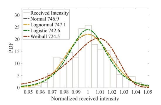
Figure 7.
PDF with various fitting distributions.
Figure 8 shows the effects of the three turbulence properties on the UWOC channel. A more dispersed distribution means more severe light fluctuation in time domain and stronger turbulence. These results are consistent with the previous conclusion gleaned from Figure 6 regarding the turbulence properties in space domain.
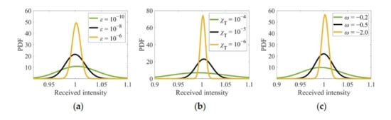
Figure 8.
Simulated PDFs with different turbulence values of (a), (b), and (c).
Figure 9 shows the influence of flow velocity, absorption and scattering, and transmission distance on the UWOC channel. In view of the almost overlapping PDFs with and in Figure 9a, the velocity of the water flow has no effect on laser transmission when all the parameters are within the predetermined range. However, the aggravation of absorption and scattering effects in Figure 9b or the extension of distance in Figure 9c will significantly reduce the mean value of the PDF, and the reduction is positively correlated with the distance and coefficients.
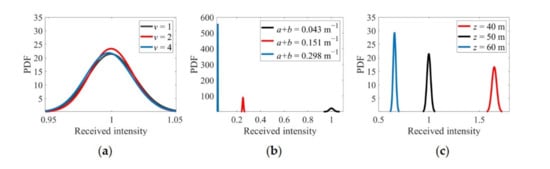
Figure 9.
Simulated PDFs with different (a) flow velocities, (b) absorption and scattering coefficients, and (c) transmission distances.
4.3. Average Intensity and Scintillation Index of the Received Light
Based on the above discussions, the channel parameters can be divided into two types: the parameters that primarily affect the average light intensity , and the parameters that primarily induce light fluctuations, which can also be characterized by the scintillation index (SI) as [31]. According to the definition of lognormal distribution, the mean value of the simulated PDF is equal to the average light intensity and its variance is equal to the [12].
In Figure 10, the average received light intensity is depicted for various absorption and scattering coefficients and transmission distances. The results calculated from eight groups of 288 simulation realizations show that the light will attenuate as the transmission distance or the seawater coefficients increase.
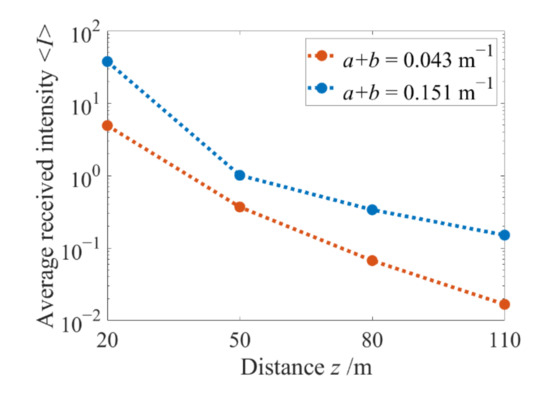
Figure 10.
Average received light intensity versus the transmission distance with different absorption and scattering coefficients.
Figure 11 illustrates the relationships between the scintillation index of the received light and the turbulence properties , the flow velocity and the transmission distance. The scintillation will intensify as the rate of dissipation of kinetic energy decreases, the rate of dissipation of mean-squared temperature increases, and the ratio approaches 0. The extension of transmission distance cause not only attenuation, but also spatial and temporal fluctuations of the light intensity, whether in the UWOC channel with turbulence or with attenuation effects.
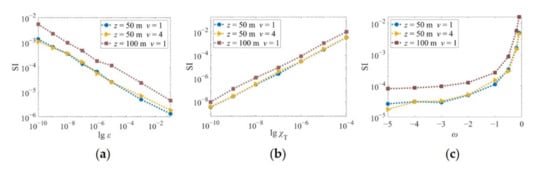
Figure 11.
Light scintillation index versus (a) , (b) , and (c) with different flow velocities and transmission distances.
4.4. BER Performance of the UWOC System
Figure 12 shows the BER performance with various attenuation coefficients, turbulence properties, and transmission distances. The BER will increase as the absorption and scattering coefficients () increase, the rate of dissipation of kinetic energy decreases, the rate of dissipation of mean-squared temperature increases, the approach of the ratio towards 0, and the transmission distance extends.
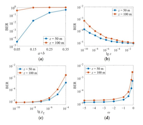
Figure 12.
BER versus (a), (b) , (c) , and (d) with different transmission distances.
Turbulence strength can be quantitatively defined with reference to the BER data in Figure 12b–d. Here, we consider weak turbulence as , , ; medium turbulence as , , ; strong turbulence as , , . We also consider three groups of absorption and scattering values [13]: and for pure seawater; and for ocean water; and for coastal water. Using these quantitative definitions, the effects of absorption, scattering, and turbulence on the UWOC performance can be analyzed comprehensively.
As illustrated in Figure 13, the BER performance will get worse with the intensification of the turbulence strength and the variation of the water quality. In coastal water or under strong turbulence, the BER is too poor to meet the forward error correction requirement. This deterioration can be partly compensated by increasing the transmitting light power. In our study, the transmission distance is 50 m and the AWGN intensity of the UWOC system is −10 dBm. Under weak turbulence in pure seawater, the BER is below 10−6 with a transmitting power higher than 0.7 dBm, but it becomes about 10−2 under medium turbulence in ocean water. By increasing the transmitting power to 7.5 dBm, the BER can return to 10−6. With the BER threshold of 10−6, the power penalty for changing pure seawater to ocean water is 5.8 dBm under weak or medium turbulence. The power penalty for changing weak turbulence to medium turbulence is 1.0 dBm in pure seawater or in ocean water. However, the increase of the light power will synchronously increase the turbulence-caused scintillation and the corresponding noise, so the power compensation will become invalid and can no longer improve the BER when the turbulence is excessively strong, that is, when the scintillation noise is dominant.
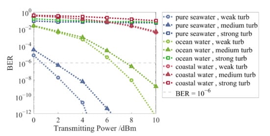
Figure 13.
BER of the UWOC system under different absorption, scattering, and turbulence conditions.
5. Conclusions
A comprehensive multiparameter model for the UWOC channel has been established by integrating the Beer-Lambert law and Monte Carlo phase screens into the split-step propagation framework, so the effects of absorption, scattering, and turbulence underwater can be evaluated simultaneously. In the modeling process, the subharmonic method and the strict sampling constraint method have been applied in combination to improve the modeling accuracy to 96.19% in line with the theoretical statistics.
The underwater optical channel is impacted by the attenuation caused by absorption and scattering effects, and the fluctuation caused by the underwater turbulence. The light scintillation becomes severer with the decrease of the dissipation rate of the turbulence kinetic energy, the increase of the temperature gradient of water, and the increase of turbulence contributions from salinity than temperature. The extension of transmission distance will aggravate both the attenuation and the fluctuation of light.
Furthermore, the BER performance is simulated for the UWOC system and it can be effectively compensated by increasing the transmitting light power when the turbulence strength is within a certain range. The power compensation method will become invalid when the turbulence is excessively strong. The power penalty of a 50 m UWOC channel is around 5.8 dBm from pure seawater to ocean water and around 1.0 dBm from weak turbulence to medium turbulence, with the BER threshold of 10−6. The proposed model can help in analyzing the effects of real underwater channels and evaluating the performance of the UWOC systems.
Author Contributions
Conceptualization, D.D. and S.G.; Investigation, R.C. and M.Z.; Methodology, R.C.; Project administration, D.D.; Resources, M.Z. and Y.S.; Software, R.C.; Supervision, S.G.; Validation, M.Z.; Visualization, R.C.; Writing—original draft, R.C.; Writing—review & editing, Y.S. and S.G. All authors will be informed about each step of manuscript processing including submission, revision, revision reminder, etc. via emails from our system or assigned Assistant Editor. All authors have read and agreed to the published version of the manuscript.
Funding
This research was funded by the National Natural Science Foundation of China (61875172), the Zhejiang Provincial Natural Science Foundation of China (LD19F050001), the Fundamental Research Funds for the Central Universities (2020XZZX005-07), and the National Key Research and Development Program of China (2019YFB2205202).
Institutional Review Board Statement
Not applicable.
Informed Consent Statement
Not applicable.
Data Availability Statement
Not applicable.
Acknowledgments
The author acknowledges the valuable comments of the reviewers.
Conflicts of Interest
The authors declare no conflict of interest.
References
- Zeng, Z.; Fu, S.; Zhang, H.; Dong, Y.; Cheng, J. A Survey of Underwater Optical Wireless Communications. IEEE Commun. Surv. Tutor. 2017, 19, 204–238. [Google Scholar] [CrossRef]
- Pompili, D.; Akyildiz, I.F. Overview of Networking-Protocols for Underwater Wireless Communications. IEEE Commun. Mag. 2009, 47, 97–102. [Google Scholar] [CrossRef]
- Khalighi, M.A.; Gabriel, C.; Hamza, T.; Bourennane, S.; Leon, P.; Rigaud, V. Underwater Wireless Optical Communication; Recent Advances and Remaining Challenges. In Proceedings of the 2014 16th International Conference on Transparent Optical Networks (ICTON), Graz, Austria, 6–10 July 2014. [Google Scholar] [CrossRef]
- Hanson, F.; Radic, S. High bandwidth underwater optical communication. Appl. Opt. 2008, 47, 277–283. [Google Scholar] [CrossRef]
- Li, Y.; Safari, M.; Henderson, R.; Haas, H. Optical OFDM with Single-Photon Avalanche Diode. IEEE Photonics Technol. Lett. 2015, 27, 943–946. [Google Scholar] [CrossRef]
- Oubei, H.M.; Duran, J.R.; Janjua, B.; Wang, H.Y.; Tsai, C.T.; Chi, Y.C.; Ng, T.K.; Kuo, H.C.; He, J.H.; Alouini, M.S.; et al. 4.8 Gbit/s 16-QAM-OFDM transmission based on compact 450-nm laser for underwater wireless optical communication. Opt. Express 2015, 23, 23302–23309. [Google Scholar] [CrossRef]
- Liu, X.; Yi, S.; Zhou, X.; Fang, Z.; Qiu, Z.J.; Hu, L.; Cong, C.; Zheng, L.; Liu, R.; Tian, P. 34.5 m underwater optical wireless communication with 2.70 Gbps data rate based on a green laser diode with NRZ-OOK modulation. Opt. Express 2017, 25, 27937–27947. [Google Scholar] [CrossRef]
- Wu, T.C.; Chi, Y.C.; Wang, H.Y.; Tsai, C.T.; Lin, G.R. Blue Laser Diode Enables Underwater Communication at 12.4 Gbps. Sci. Rep. 2017, 7, 40480. [Google Scholar] [CrossRef]
- Fei, C.; Hong, X.; Zhang, G.; Du, J.; Gong, Y.; Evans, J.; He, S. 16.6 Gbps data rate for underwater wireless optical transmission with single laser diode achieved with discrete multi-tone and post nonlinear equalization. Opt. Express 2018, 26, 34060–34069. [Google Scholar] [CrossRef]
- Shen, J.; Wang, J.; Chen, X.; Zhang, C.; Kong, M.; Tong, Z.; Xu, J. Towards power-efficient long-reach underwater wireless optical communication using a multi-pixel photon counter. Opt. Express 2018, 26, 23565–23571. [Google Scholar] [CrossRef]
- Duntley, S.Q. Light in the Sea. J. Opt. Soc. Am. 1963, 53, 214–233. [Google Scholar] [CrossRef]
- Che, X.; Wells, I.; Dickers, G.; Kear, P.; Gong, X. Re-Evaluation of RF Electromagnetic Communication in Underwater Sensor Networks. IEEE Commun. Mag. 2010, 48, 143–151. [Google Scholar] [CrossRef]
- Cochenour, B.M.; Mullen, L.J.; Laux, A.E. Characterization of the Beam-Spread Function for Underwater Wireless Optical Communications Links. IEEE J. Ocean. Eng. 2008, 33, 513–521. [Google Scholar] [CrossRef]
- Johnson, L.; Green, R.; Leeson, M. A survey of channel models for underwater optical wireless communication. In Proceedings of the 2013 2nd International Workshop on Optical Wireless Communications (IWOW), Newcastle Upon Tyne, UK, 21 October 2013. [Google Scholar] [CrossRef]
- Li, C.; Park, K.H.; Alouini, M.S. On the Use of a Direct Radiative Transfer Equation Solver for Path Loss Calculation in Underwater Optical Wireless Channels. IEEE Wirel. Commun. Lett. 2015, 4, 561–564. [Google Scholar] [CrossRef] [Green Version]
- Yang, Y.; He, F.; Guo, Q.; Wang, M.; Zhang, J.; Duan, Z. Analysis of underwater wireless optical communication system performance. Appl. Opt. 2019, 58, 9808–9814. [Google Scholar] [CrossRef]
- Hanson, F.; Lasher, M. Effects of underwater turbulence on laser beam propagation and coupling into single-mode optical fiber. Appl. Opt. 2010, 49, 3224–3230. [Google Scholar] [CrossRef]
- Zhang, J.; Kou, L.; Yang, Y.; He, F.; Duan, Z. Monte-Carlo-based optical wireless underwater channel modeling with oceanic turbulence. Opt. Commun. 2020, 475, 126214. [Google Scholar] [CrossRef]
- Martin, J.M.; Flatté, S. Simulation of point-source scintillation through three-dimensional random media. J. Opt. Soc. Am. A 1990, 7, 838–847. [Google Scholar] [CrossRef]
- Lukin, V.P.; Fortes, B.V. Laser Beam Propagation in the Atmosphere. In Adaptive Beaming and Imaging in the Turbulent Atmosphere; SPIE Press: Bellingham, WA, USA, 2002; ISBN 0819443379. [Google Scholar]
- Yu, N.; Genevet, P.; Kats, M.A.; Aieta, F.; Tetienne, J.P.; Capasso, F.; Gaburro, Z. Light propagation with phase discontinuities: Generalized laws of reflection and refraction. Science 2011, 334, 333–337. [Google Scholar] [CrossRef] [Green Version]
- Bissonnette, L.R.; Welsh, B.M.; Dainty, C. Fourier-series-based atmospheric phase screen generator for simulating anisoplanatic geometries and temporal evolution. Proc. SPIE Int. Soc. Opt. Eng. 1997, 3125, 327–338. [Google Scholar] [CrossRef]
- Nikishov, V.V.; Nikishov, V.I. Spectrum of turbulent fluctuations of the sea-water refraction index. Int. J. Fluid Mech. Res. 2000, 27, 82–98. [Google Scholar] [CrossRef]
- Thormählen, I.; Straub, J.; Grigull, U. Refractive Index of Water and Its Dependence on Wavelength, Temperature, and Density. J. Phys. Chem. Ref. Data 1985, 14, 933–945. [Google Scholar] [CrossRef] [Green Version]
- Dios, F.; Recolons, J.; Rodriguez, A.; Batet, O. Temporal analysis of laser beam propagation in the atmosphere using computer-generated long phase screens. Opt. Express 2008, 16, 2206–2220. [Google Scholar] [CrossRef] [Green Version]
- Mobley, C.D.; Gentili, B.; Gordon, H.R.; Jin, Z.; Kattawar, G.W.; Morel, A.; Reinersman, P.; Stamnes, K.; Stavn, R.H. Comparison of numerical models for computing underwater light fields. Appl. Opt. 1993, 32, 7484–7504. [Google Scholar] [CrossRef] [PubMed] [Green Version]
- Schmidt, J.D. Fresnel Diffraction in Vacuum. In Numerical Simulation of Optical Wave Propagation: With Examples in MATLAB; SPIE: Bellingham, WA, USA, 2010; pp. 87–113. [Google Scholar] [CrossRef]
- Lane, R.G.; Glindemann, A.; Dainty, J.C. Simulation of a Kolmogorov phase screen. Waves Random Media 2006, 2, 209–224. [Google Scholar] [CrossRef]
- Lu, L.; Ji, X.; Baykal, Y. Wave structure function and spatial coherence radius of plane and spherical waves propagating through oceanic turbulence. Opt. Express 2014, 22, 27112–27122. [Google Scholar] [CrossRef] [PubMed]
- Schmidt, J.D. Propagation through Atmospheric Turbulence. In Numerical Simulation of Optical Wave Propagation with Examples in MATLAB; SPIE: Bellingham, WA, USA, 2010; pp. 149–184. [Google Scholar] [CrossRef]
- Korotkova, O.; Farwell, N.; Shchepakina, E. Light scintillation in oceanic turbulence. Waves Random Complex Media 2012, 22, 260–266. [Google Scholar] [CrossRef]
Publisher’s Note: MDPI stays neutral with regard to jurisdictional claims in published maps and institutional affiliations. |
© 2021 by the authors. Licensee MDPI, Basel, Switzerland. This article is an open access article distributed under the terms and conditions of the Creative Commons Attribution (CC BY) license (https://creativecommons.org/licenses/by/4.0/).