Abstract
The use of an inconsistent speed limit determination method can cause low speed limit compliance. Therefore, we developed an objective methodology based on engineering judgment considering the traffic accident rate in road sections, the degree of roadside development, and the geometric characteristics of road sections in urban roads. The scope of this study is one-way roads with two or more lanes in cities, and appropriate sections were selected among all roads in Seoul. These roads have speed limits of the statutory maximum speed of 80 km/h or lower and are characterized by various speeds according to the function of the road, the roadside development, and traffic conditions. The optimal speed limits of urban roads were estimated by applying the characteristics of variables as adjustment factors based on the statutory maximum speed limit. As a result of investigating and testing various influence variables, the function of roads, the existence of median, the level of curbside parking, the number of roadside access points, and the number of traffic breaks were selected as optional variables that influence the operating speed. The speed limit of one-way roads with two or more lanes in Seoul was approximately 10 km/h lower than the current speed limit. The existing speed limits of the roads were applied uniformly considering only the functional road class. However, considering the road environment, the speed limit should be applied differently for each road. In the future, if the collection scope and real-time collection of road environment information can be determined, the GIS visualization of traffic safety information will be possible for all road sections and the safety of road users can be ensured.
1. Introduction
1.1. Background and Objectives of Study
In South Korea, 72.1% of traffic accidents and 51.2% of total deaths occurred on urban roads during the past five years (2010–2015) [1]. The annual growth rate of accidents was 1.31% in cities, which is higher than the rate of 0.45% for the whole country. The decrease in the rate of the deaths was 0.22% in cities, lower than the decrease of 3.44% for the whole country.
During the past 10 years (2004–2013) [2], 38% of the total number of traffic deaths in 27 countries of the EU occurred in cities. During the same period, while the number of deaths decreased by approximately 42% the ratio of deaths in cities increased slightly.
Compared to these countries, South Korea has a high ratio of traffic deaths in cities (51.2%), while the decrease rate of deaths in cities is low. Thus, cities and provinces need to make efforts to reduce the incidence traffic accidents.
The 8th National Traffic Safety Basic Plan (2017–2021, Ministry of Land, Infrastructure, and Transport) presents speed control reinforcement measures as a traffic safety promotion strategy. Specifically, the ministry plans to lower the urban speed limits to 50 km/h in principle and to expand roads with 30 km/h or lower speed limits.
Although such policy efforts for traffic safety are timely, there is a problem in that there is no method by which traffic officials in charge of speed control can set a specific speed limit in the field. Since urban roads have various functions and roadside conditions, if the officials in charge establish speed limits based on their experience, intuition, or civil petitions, it is difficult to secure the justification for speed control due to the lack of concrete grounds for it, and decreased confidence in the speed limit can contribute to low compliance rates.
The objective of this study is to develop a model that can be used by traffic officials to easily estimate the optimal speed limit based on objective grounds when they want to establish speed limits for urban road sections using vehicle traffic information big data, as well as to estimate the traffic accident reduction effect.
1.2. Content and Method of Study
A novel method of calculating the speed limit using the traffic volume, road environment information, and accident data was developed to improve the method of calculating the speed limit based on the functional road class.
The subject roads are one-way roads with two or more lanes in Seoul. The contents and process of this study are outlined in Figure 1.
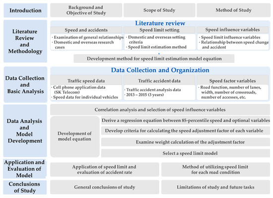
Figure 1.
Process of the study.
We selected variables that affect the driving speed and developed a speed limit calculation model equation using the correlation between different variables and the development of the adjustment factor of each variable. We also evaluated the effect of the calculated speed limit by applying the effect prediction method presented in the literature.
2. Theory and Prior Studies
2.1. Speed Limit Setting Criteria
2.1.1. Korean Criteria
Article 17, Paragraph 1 of the current Road Traffic Act (28 July 2016), and Article 19, Paragraph 1 of the Enforcement Rule of the same act specify that the statutory maximum speed limit is 60 km/h on general roads, and 80 km/h or less on one-way roads with two or more lanes. The current statutory maximum speed limits in South Korea shown in Table 1.

Table 1.
Current statutory maximum speed limits in South Korea.
2.1.2. Overseas Criteria
In Australia, the speed limit for urban arterial roads is 60 km/h in general. However, speed limits of 60 km/h or higher are not generally used in many OECD countries, and 50 km/h is widely used instead. The speed limit is generally 50 km for collector and local roads, and many OECD countries use a limit of 30~40 km/h [3]. The detailed speed limit by country is shown in Table 2.
Table 2.
General speed limits in OECD countries.
Most OECD/ITF [4] countries use 50 km/h as the default speed limit for passengers in cities. Low speed limits (typically 30 km/h) are applied to residential areas and near schools. The default speed limit of 60 km/h is applied in Poland, Chile, and South Korea.
Japan [5] established speed regulation standards (12 standards) for general roads in 2009, considering the three factors of traffic accident risk, the existence of median, and pedestrian protection in urban areas based on the results of the “Study on the direction of speed limit decision” in 2009.
The U.S. abolished the 55 mph maximum speed limit, which had been enforced by the federal government since 1974 (April 1995), and delegated authority to state governments so that they could define the speed limits for all roads (urban and regional) (TRB: Transportation Research Board, 1998) [6].
Sweden (WHO, 2008) [7] has set speed limits to prevent deaths and injuries based on the philosophy of ‘Vision zero’ since the 1960s and is benchmarked in Europe as a good example of speed limit establishment.
The WHO (2013, 2015) [8,9] reported that 97 out of 180 countries around the world have urban maximum speed limits equal to or lower than 50 km/h and emphasizes that more countries should introduce 50 km/h as the maximum speed based on its accident reduction effect. In these countries, higher speed limits are applied as an exception to some roads such as urban belt highways. The following Figure 2 shows the classification of the speed limit by country/area.
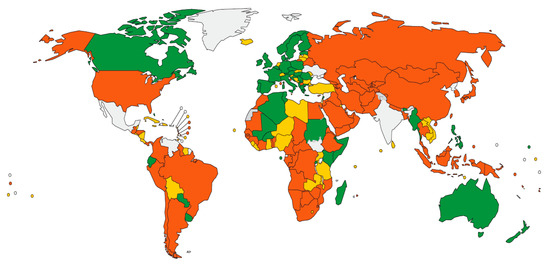
Figure 2.
Urban speed limits by country/area.
2.2. Speed Limit Estimation Method
The general speed limit method applies the statutory speed limit to many types of roads and the speed zoning method to roads for which the limit is not appropriate.
2.2.1. Engineering Study Methods
Operating speed method: Most engineering study methods belong to this category. The speed limit is determined based on the 85th percentile speed first and then adjusted in accordance with the traffic conditions and geometric structures. This method is applied to many regional roads.
Forbes et al. [10] stated that the 85th percentile speed reflected the collective judgment that most drivers choose a reasonable speed for the given traffic and road conditions.
Road risk method: This is another engineering study method that sets the speed limit based on the risks associated with the road geometric design and traffic conditions. This method is mainly used in Canada and New Zealand [10].
2.2.2. Optimal Speed Limits
This method was proposed in 1962 by Oppenlander to scientifically limit the vehicle travel speed so that it will be optimal from the social perspective. The speed limit that minimizes socio-economic costs is determined by considering the environmental cost, accident cost, travel time, fuel consumption, etc., so that the travel speed chosen will be optimal in terms of social costs and benefits.
Hossseinlou et al. [11] reported that the optimal speed limit for expressways in Iran from the social perspective was 10 km/h lower than the optimal speed limit from the driver perspective and suggested the following relationship:
Optimal speed limit ≤ maximum speed limit ≤ design speed.
2.2.3. Expert System Approach
This approach determines the speed limit with a computer program using the knowledge base and an inference procedure that simulates the behaviors and judgment of experts. It was first implemented by the Victoria State in Australia in 1987 to create a unified, consistent approach to determining section speed limits.
The U.S. uses an expert system (USLIMITS2) [12] to determine the optimal speed limits in “speed zones”. As a web-based expert advisor system, when data are provided through a user program, it outputs the recommended speed limit and cautions for the given conditions, thus playing an assistive role in setting an appropriate speed limit.
2.2.4. Injury Minimization Approach
This approach determines the speed limit based on the vehicle crash tolerance of the human body. The basic objectives of this method are to set the speed limit to a speed that does not expose users to crash risks that could cause death or serious injuries and prevent cars from traveling above the speed. The speed limit that minimizes injuries by road type is shown in Table 3.
Table 3.
Speed limits for injury minimization.
Different speed limit estimation methods are compared in Table 4. In this study, we applied the engineering (operating speed) method.
Table 4.
Approaches to setting a speed limit.
2.3. Speed and Traffic Safety
The accident rate increases with the speed dispersion, and the speed dispersion tends to become minimized when the difference between the design speed and the speed limit is between 5 and 10 mph on all road types [13,14].
In the relationship between speed and accident rate, the accident rate increases as the speed becomes lower or higher, and the number of accidents causing injuries and property damage increases exponentially with the speed [15,16,17].
The relationship between speed and the number of accidents is either a simple linear relationship or a weak curve function. If the speed is higher or lower than the mean traffic speed, the accident rate increases or decreases proportionally, and the vehicles driving at the mean traffic speed do not have any advantage [18].
High speed means more accidents, and the higher the speed, the faster the frequency of accidents increases with the speed [19,20].
When the mean speed increases by 5%, all injury accidents increase by 10% and fatal accidents increase by 20%; when the mean speed decreases by 5%, the number of accidents causing injuries decreases by 10% and the number of fatal accidents decreases by 20% [21].
The number of accidents causing property damage changes similarly even with small changes in the travel speed, but fatalities increase at four times the rate of speed change [22,23,24,25].
2.4. Motivation and Differentiation of Research
To summarize the related research, travel speed and traffic environment information is needed to estimate the speed limit according to the road and traffic conditions. If the appropriate speed limit is estimated for the road situation, the vehicle-specific speed deviation decreases, reducing the likelihood of traffic accidents occurring.
However, the existing research relating to selecting a speed limit has not developed due to the limitations of data collection, and some methods select the speed limit only according to the function of the road. As shown in Figure 3, since detectors are installed only on some roads, it is not possible to collect data on all urban roads. This is a problem not only in Korea, but in all countries.
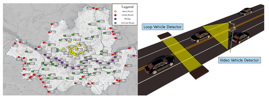
Figure 3.
Location and collection method of traffic detectors in Seoul.
Due to the limitations of detectors’ collection space and accuracy, until now, the total traffic volume of a city was predicted using loop detector data and studies aiming to improve the accuracy were conducted [26,27].
Recently, it has become possible to acquire driving information for each driver (speed, location, route, etc.) using cell phones, and the method of collecting the data has also changed. When application collection data are applied to GIS, they can be applied as traffic volume and speed data, as shown in Figure 4.
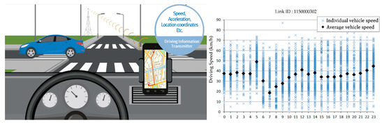
Figure 4.
Real-time driving information collection using cell phone data transmission.
However, the road environment information that affects the speed limit is not managed as a DB by the road management agency. Therefore, geometry data are obtained by collecting data through sample field surveys (72 sections).
When integrating the collected data, as shown in Figure 5, it is possible to provide a safe speed limit considering the road geometry and traffic characteristics rather than applying the existing uniform speed limit.
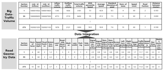
Figure 5.
Big data integration and parameter setting.
Therefore, this study aimed to develop a speed limit estimation model equation by analyzing application-collected data and field survey data from urban roads (one-way roads with two or more lanes and a speed limit of 80 km/h or less) in Seoul.
3. Data Collection and Model Equation Development
3.1. Research Methodology
3.1.1. Basic Concept and Procedure
This study was based on “the speed zoning method” [28]. The function was modified by adding roadside conditions based on the 85th percentile speed as follows:
where RSL is recommended speed limit (km/h); MSSL is maximum statutory speed limit (80 km/h); and fi is factor for adjusting the effects of roadside conditions (based on the calculation of the adjustment factor).
RSL = MSSL × f1 × f2 × f3 ×, … ×, fi,
To establish the relationships between the 85th percentile speed and various variables in a “safe section”, road sections were selected according to the following criteria:
- The sections must have a low accident rate;
- The sections must have a low standard deviation with respect to traffic flow.
The process for the development of the speed limit estimation model equation is illustrated in Figure 6.
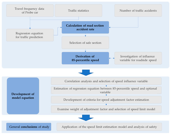
Figure 6.
Speed limit estimation model development process.
3.1.2. Development of Adjustment Factor Estimation Criteria
To develop the adjustment factor estimation criteria, it was first assumed that a variable (Vi) and its corresponding adjustment factor (fi) have a linear relationship. Figure 7 shows an abbreviated form of fi between 0 and 1 on the y-axis. In addition, the x-axis variable was standardized to a value between 0 and 1. Then, if the standardized variable is denoted as SVi, the adjustment factor can be obtained as follows:
where s νi is standardized variable i.
fi = 1 − s νi,
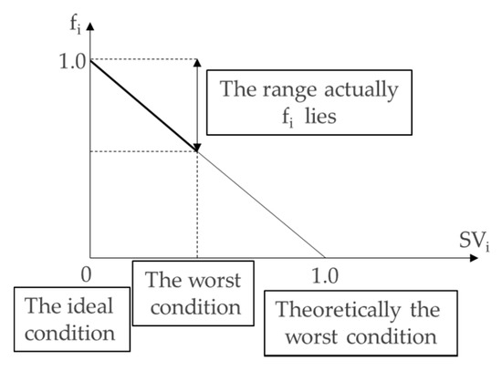
Figure 7.
Framework for adjustment factor module design.
Variables can be either continuous or categorical, and the fi–SVi relationship illustrated in Figure 8 can be used according to the variable (Figure 8a shows a discrete categorical variable, while Figure 8b shows two or more categorical variables).
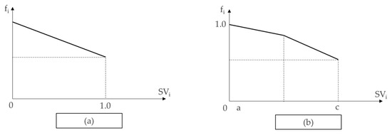
Figure 8.
Alternative forms of the adjustment factor module.
3.1.3. Variable Standardization
To convert the value of a given variable to a factor value between 0 and 1, the 85th percentile speed and linear estimation function were obtained for each variable (Figure 9). The objective of the function estimation is to determine the statistical significance (i.e., p = 0.05) and obtain a linear relationship.
where fij is the adjustment factor of variable j at section I; Vij is the coefficient of variable j at section I; and αi is the slope from the linear regression estimation equation.
fij = 1 − (νij × αi)/80,
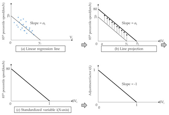
Figure 9.
Plots illustrating the standardization procedure.
3.1.4. Weighting Factors
The purpose of the weighting factor is to establish the relative importance level of each variable in the above model. With the weighting factors incorporated, the speed limit estimation model equation is expressed as:
where wi is weight for calculating other effects of the variable in the model equation.
RSL = 80 km/h × [1 − (ν1j × αi)/80]w1 × [1 − (ν2j × α2)/80]w2 × [1 − (ν3j × α3)/80]w3 ×,⋯,× [1 − (νij × αi)/80]wi,
3.1.5. Model Test and Utilization
When calculating the optimal speed limits for many accident points according to the completed model, if the difference between the actual 85th percentile speed (V85) and the speed limit (RSL) is large in a section where many accidents occur, the speed limit can be considered unsafe.
3.2. Data Collection
The development of the speed limit estimation model involves data collection and analysis stages, as illustrated in Figure 10. Of the 215 sections surveyed, 36 “safe road sections” with low accident rates and standard deviations were selected.
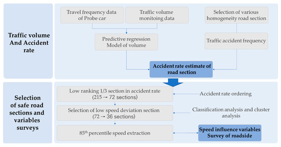
Figure 10.
Describing the data collection and analysis stages.
3.2.1. Road Section Traffic Volumes
To estimate the accident rate in order to select safe road sections, we used Seoul traffic volume statistics [29] and the traffic volumes recorded by cell phone applications, containing travel speed data for individual drivers (Table 5). The traffic volume by link is shown in Figure 11. For the travel speed data, the raw cell phone application data were converted to match them with the national standard ITS link.
Table 5.
Operating speed data conversion and corresponding form.
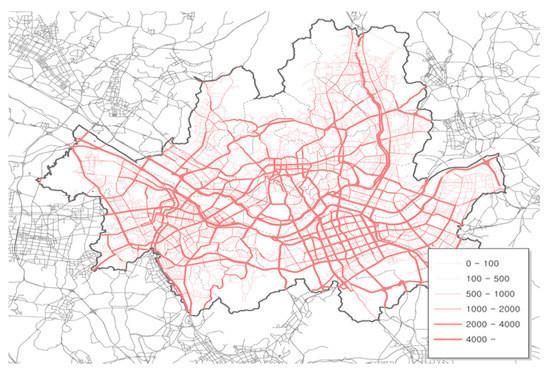
Figure 11.
Traffic volume distribution in Seoul using cell phone application data (veh./day).
A previous weighted regression analysis by Kim et al. [30] considered 58 annual average daily traffic volume (AADT) survey points and the traffic volumes of vehicles with navigation systems (R2 = 0.835), with the model equation demonstrating a high goodness of fit and a reliable coefficient (p < 0.001). The constant and regression coefficient were estimated to be 10,676 and 8.368, respectively.
3.2.2. Selection of Road Sections
The road section selection criterion used in this study was based on traffic breaks, that is, road sections with relatively uniform traffic characteristics. The speed limit and number of lanes were also considered. After selecting sections considered to be homogeneous roads in each district in Seoul, detailed data were collected from Internet map sites. As road design factors were not considered in this study, we selected uniform road sections with a minimum length of 800 m and without distinct slopes (FHWA, 2012). The detailed number of road sections and Distances are shown in Table 6.
Table 6.
Numbers of road sections and their total distance for different Seoul districts.
3.2.3. Estimation of Accident Rate by Road Section
To select safe road sections, accident rates were estimated using accident data for the three-year period from 2013 to 2015 and the abovementioned estimated traffic volume data. The accident data were collected through a geographic information system analysis of traffic accidents in the traffic accident analysis system (TAAS) of the National Police Agency.
To estimate the accident rate per 100 million vehicles, we followed the method described in [31]. The estimated result is shown in Figure 12.
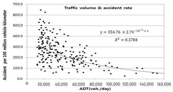
Figure 12.
Accident rate as a function of the average daily traffic volume.
3.2.4. Selection of Safe Road Sections
After ranking the estimated accident rates, the third of the sections (72 sections) with the lowest accident rates were selected as safe road sections. After selecting the sections with low accident rates, the road sections with small standard deviations for a group of vehicles with a stable traffic flow were selected.
3.2.5. Extracting Speed Data
In general, the 85th percentile speed is a spot speed measured in free-flowing traffic conditions for which the prevailing speed in clear weather conditions during the daytime is measured and recorded on weekdays [32]. The speed data in this study were used to identify the extent to which speed-related variables influence the speed under certain conditions. The following sections were selected for the speed survey:
The first condition informs estimations of the driving speed, while excluding the effects of signals described by Jeong [33]. The second condition is applied to minimize the effect of traffic jams by identifying the duration at which traffic flowed at the average maximum travel speed for each road section.
3.2.6. Variables Related to Roadside Speed
The numerous (integrated) road variables affecting speed that have been investigated in related literature [34,35] are listed in Table 7.
Table 7.
Speed affecting variables investigated in the literature.
3.3. Correlation Analysis and Variable Selection
The criteria deployed in the correlation analysis of variables known to affect speed limit determination are listed in Table 8.
Table 8.
Correlation coefficient criteria.
In this study, a correlation coefficient of 0.4 was set as the threshold to differentiate between dependent and independent variables, while 0.4–0.6 was set as the threshold to differentiate between moderate and strong correlation. To determine whether a particular variable could be used as a determinant in the proposed speed limit model, a p-value of 0.05 was applied to evaluate its significance.
The full results are listed in Table 9, with the regression analysis results of the selected five variables summarized in Table 10.
Table 9.
Correlation coefficients between the main variables.
Table 10.
Regression analysis results for selected variables.
3.4. Development of Adjustment Factor Estimation Criteria
To develop the adjustment factor estimation criteria, the relationship between the adjustment factors (fi) corresponding to a variable (Vi) was assumed to be linear.
For convenience, we adopted a variable notation when applying estimation criteria, as described in Table 11.
Table 11.
Variable abbreviations.
3.4.1. The Adjustment Factor (fRFC) Pertaining to the Road Function
The adjustment factor (fRFC) pertaining to the road function is a categorical variable and was classified by road type—(1) arterial roads, (2) auxiliary arterial roads, and (3) collector roads—and estimated to be similar to the binomial optional variable. The estimated slope in the regression equation was −5.11, while the constant was estimated to be 61.10:
85th percentile speed = 61.10 − 5.11 × VRFC.
The slope represents the sensitivity of the road function for the 85th percentile speed. Arterial and collector roads were found to have adjustment factors of 1.0 and 0.87, respectively:
(69.78 km/h × 1.00)/80 km/h = 0.87.
Therefore, to standardize the x-axis in the 0–1 range, we used the following expression:
where VRFC represents arterial, auxiliary arterial, and collector roads accordingly. The estimation process is expressed in a graph, as shown in Figure 13.
fRFCj = 1.00 − 0.13 × (VRFCj − 1)/2,
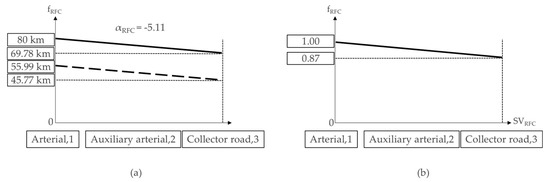
Figure 13.
Adjustment factor development (a) and standardization for the existence (b) of road function.
3.4.2. The Adjustment Factor (fCD) Pertaining to the Median Strip
The existence of median is a discrete optional variable with an estimated slope of 14.68 and a constant of 49.98. If there is a median for the 85th percentile speed, the dotted line moves together with the solid line so that it becomes 80 km/h and has the same slope and constant for the y-axis. The standardization constant for y-axis is 0.82 and the median adjustment factor fCD for the last survey section j can be expressed as follows:
(65.32 km/h × 1.00)/80 km/h = 0.82.
Therefore, when it is standardized for the x-axis so that it will become 1.0,
where VCDj is 1 if there is a median and 0 otherwise.
FCDj = 0.82 + 0.18 × (VCDj),
The estimation process is expressed in a graph, as shown in Figure 14.
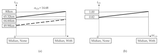
Figure 14.
Adjustment factor development (a) and standardization for the existence (b) of the median strip.
3.4.3. The Adjustment Factor (fPL) Pertaining to the Level of Parking
The adjustment coefficient for parking density is calculated in the same way as the road functional class, with the adjustment factor (fPL) expressed as:
where VPL = 1 if the level of parking is almost zero, 2 if it is low, and 3 if it is high.
(67.38 km × 1.00)/80 km/h = 0.84,
FPLj = 1.00 − 0.16 × (VPLj − 1)/2,
The estimation process is expressed in a graph, as shown in Figure 15.
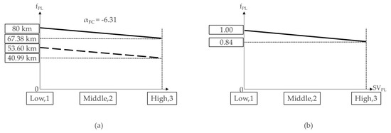
Figure 15.
Adjustment factor development (a) and standardization for the existence (b) of the level of parking.
3.4.4. The Adjustment Factor (fAD) Pertaining to the Number of Access Density
The number of access points (VAD) and the adjustment factor are constant for both the x- and y-axes. The larger the number of access points is, the lower the speed is. The slope estimated by the regression equation (αAD) was −0.36, corresponding to a constant of 58.63.
As described earlier, the constant (yAD) for the x-axis is 162.9. If the estimated regression line is projected to be 80 km, the constant (δAD) corresponding to the x-axis is. Thus, when the total number of access points per km is approximately, the travel speed, in theory, becomes zero:
85th percentile speed = 58.63 − 0.36 × VAD,
δAS = 80/αAD = 80/0.36 = 222.2.
Next, we obtain the standardization value corresponding to the observed number of access roads:
where SVADj denotes the standardized number of access points for the jth section, VADj denotes the number of access points for the jth section, and δAD is the x-axis constant corresponding to the 80 km projected line.
SVADj = VADj/δAD, fADj = 1.0 − SVADj = 1.0 − (VADj/δAD),
Using the above equation, the adjustment factor according to the number of access points in the jth section is calculated as:
fADj = 1.0 − (VADj × αAD)/80 = 1.0 − (VADj/222.2).
The estimation process is expressed in a graph, as shown in Figure 16.
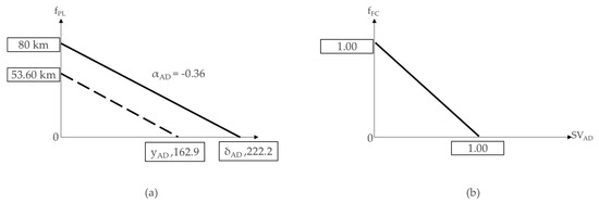
Figure 16.
Adjustment factor development (a) and standardization for the existence (b) of the number of access density.
3.4.5. The Adjustment Factor (fSD) Pertaining to the Number of Traffic Breaks
The adjustment factor for the number of traffic breaks (VSD) is obtained via the same process. The larger the number of traffic break facilities is, the lower the travel speed is. The slope estimated by the regression equation is −2.13 and the constant is 62.53. In the following equation, the constant (ySD) for the x-axis is 29.4. When the estimated regression line is projected to be 80 km, the constant for the x-axis (δSD) is 37.6. Therefore, when the number of traffic break facilities per km is approximately, the travel speed theoretically becomes zero:
85-percential speed = 62.53 − 2.13 × VSD,
δSD = 80/αSD = 80/2.13 = 37.6.
Following this, we obtained the standardization value corresponding to the observed number of traffic break facilities:
where SVSDj denotes the standardized number of traffic break facilities for the jth section, VSDj is the number of traffic break facilities surveyed in the jth section, and δSD is the constant of the x-axis for the 80 km projected line.
SVSDj = VSDj/δSD, fSDj = 1.0 − SVSDj = 1.0 − (VSDj/δSD),
In accordance with the above equation, the adjustment factor corresponding to the number of traffic break facilities in the jth section is calculated as:
fSDj = 1.0 − (VSDj × αSD)/80 = 1.0 − (VSDj/37.6).
The estimation process is expressed in a graph, as shown in Figure 17.

Figure 17.
Adjustment factor development (a) and standardization for the existence (b) of the number of traffic breaks.
When the speed limit estimation model (see Equation (1)) is completed by combining the adjustment factor calculation equations for each variable (i.e., Equations (5)–(9)), we obtain the following equation:
where VFC is the road function (main arterial road: 1; auxiliary arterial road: 2; collector road: 3), VCD is the existence of a median strip (existence: 1; absence: 0), VPL is the parking density (low: 1; mid: 2; high: 3), VAD is the number of access points per km, and VSD is the number of traffic breaks per km.
Speed limit(RSL) = 80 × (1 − 0.13 × (VFC − 1)/2) × (0.82 + 0.18VCD) × (1 − 0.16 × (VPL − 1)/2) × (1 − VAD/222.2) × (1 − VSD/37.6),
3.5. Weighting Factors Verification
In Section 3.4, the adjustment coefficient was calculated by reflecting the relationship between each variable and V85, but the effect of each adjustment coefficient may be different in the combined model (Equation (10)). It is necessary to verify the weight calculation for each coefficient. The fact that the weight of the adjustment coefficient calculation criterion is close to 1 means that the linear assumption in the development of the calculation criterion is satisfied in the speed limit model equation.
For weight verification, if a weight (wi) is assumed in Equation (10) and a natural logarithm is taken, verification through multiple linear regression analysis is possible. To calculate the weight, the above equation is converted into a log function form according to the variables of this study, as shown in Equation (11):
ln(RSL/MSSL) = (wfc × ln[1 − 0.13 × (VFC − 1)/2]) + (wCD × ln[0.82 + 0.18VCD]) + (wPL × ln[1 − 0.16 × (VPL − 1)/2]) + (wAD × ln[1 − VAD/222.2]) + (wsd × ln[1 − VSD/37.6]).
Multiple linear regression model coefficients were estimated with ln(RSL/80) as the dependent variable and ln(fi) as the independent variable. The F-value and coefficient of determination (R2) were analyzed to examine the significance of the independent variable at the 0.05 level, find the correlation between variables, and determine whether the model is useful.
As a result of the multiple regression analysis, we determined that the model fit was high, with a coefficient of determination of 1.0, as shown in Table 12.
Table 12.
Results of the multiple regression analysis.
Since the regression coefficient value is close to 1 for all variables, it can be judged that the linear hypothesis applied when developing the calculation criteria is correct. Multicollinearity between variables is not a problem because the variance extension coefficient is also less than 1.
4. Estimation of Traffic Accident Reduction Effect and Application Method
4.1. Speed Limit Test and Comparison
The purpose of the test and comparison approach is to examine the possibility that the proposed model equation is suitable for application to road sections with a high accident rate. In the field, the speed limit is estimated in units of 10 km/h and may not lead to an actual decrease in the operating speed limit. However, there are differences in the average speed between the low (45 sections) and high (27 sections) accident rate groups. Figure 18 shows the accident rate distribution obtained by analyzing the difference between the operating speed and recommended speed limit for road sections with low, middle, and high accident rates. For the high accident rate sections, the speed limit was generally estimated to be low (large speed difference).
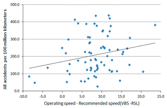
Figure 18.
Accident rate as a function of speed difference (V85-RSL).
As shown in Table 13, the test results show that the speed difference between the high and low accident rate groups follows a normal distribution, leading to the conclusion that there is no significant difference between these groups at a significance level of 0.05. However, since the significance level was 0.086 (i.e., an 8.6% probability of being equal), it can be concluded that they are different at a significance level of 0.1. This translates to the proposed speed limit estimation being lower than the current operating speed for high accident rate sections. The average estimated speed difference (PSL−RSL) across the 72 sections was 10.7 km/h, implying that the speed limit should be lowered by an average of 10 km/h relative to the current speed limit on one-way roads with two or more lanes.
Table 13.
Two-sample t-test for the speed difference (V85-RSL) between the high and low accident rate groups.
4.2. Estimation of Accident Reduction Effect
According to Elvik [36], higher driving speeds lead to the accident rate increasing according to the road type. Therefore, assuming that other conditions are maintained, if the speed limit calculated by the estimation equation is lower than the existing speed limit, it is expected that the accident rate would decrease owing to the reduction in the operating speed.
Regarding the relationship between speed limit changes and subsequent mean operating speed changes, speed limit reductions implemented using the power model resulted in a 25% reduction in the mean operating speed [37]. For example, reducing the speed limit by 10 km/h corresponded with the mean speed decreasing by 2.7 km/h (Figure 19).
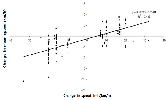
Figure 19.
Relationship between changing the speed limit and the subsequent change in mean driving speed.
Although accident severity is not reflected, it is evident that the frequency of accidents decreases in response to speed reductions (Figure 20).
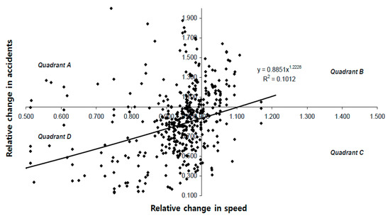
Figure 20.
Simple linear relationship between the relative change in speed and the corresponding change in accident frequency.
The anticipated relative change in accident frequency as a result of changing the relative speed is expressed as:
where y is the relative change in the accident rate and X is the relative change in speed.
y = 0.8851 × X1.2228,
When the speed limit (in 10 km units) determined by the proposed model equation is compared against the current speed limits, an average reduction of 11.1 km/h is recommended. It is expected that the mean travel speed for the analyzed road sections (47.8 km/h) would decrease by 25% with this recommended speed limit reduction (2.8 km/h; reduction rate: 0.94). The accident reduction effect corresponding to this estimated reduction in mean driving speed was calculated (using Equation (12)) as 18%.
Considering the results of the study in the context of accident severity [36,37], it is estimated that deaths would decrease by 17–24%, serious injuries by 11–17%, minor injuries by 6–9%, and property damage accidents by 5–6%.
4.3. Field Application Method
The steps followed by working officials for the estimation and implementation of speed limits in specific road sections are presented in Table 14. In addition, when applying estimated speed limits, the speed limits of nearby road sections and the proximity of sections with high accident rates should be considered.
Table 14.
Application steps and details.
If it is difficult to collect data for each branch, the results interpreted based on the data applied in this study can be used. Table 15 shows the classification of road functions and the proposed speed limits (10 km unit) into optimal groups.
Table 15.
Classification of speed limit groups according to the road environment.
5. Conclusions and Outlook
Determining the optimal speed limits that facilitate efficient and safe travel is crucial for urban roads. According to the general speed limit determination method, acting officials determine speed limits by considering whether the speed limit based on the statutory speed limit is appropriate for the characteristics of a specific road section.
To calculate the appropriate speed limit, it is necessary to take into account the road geometry [7,36] and roadside development information [35].
In previous studies, only factors related to the speed limit were classified because it was impossible to diversify the analysis section [26,27] and collect accurate driving speed information [7,36] for the driver due to the problem of the available data collection technology.
To address this, we propose an optimal speed limit estimation model for road sections based on big data regarding traffic flow statistics, environmental characteristics for urban roads, and the anticipated accident reduction effect of the developed model.
The optimal speed limit estimation method for urban roads developed in this study reflects the effects of actual roadside variables on speeds set according to the statutory maximum speed limit for one-way roads with two or more lanes.
Based on surveying and testing various influential variables, the key variables influencing the operating speed were determined as the function of the road, the existence of a median strip, the lane width, the number of roadside access points, and the number of traffic breaks.
The speed limit estimation model equation was derived by integrating the adjustment factor calculation equations for each variable.
These equations act as reduction coefficients with respect to the statutory maximum speed limit in the proposed model equation and can be changed independently depending on the optimal relationship between the variable conditions.
Validation tests show that the linear relationship between the variables assumed at the time of selecting the coefficients of the model and the speed was proven. The fit of the model is also shown to be high.
The improvement of safety aspects can be expected with the implementation of the developed model. However, the model also has some limitations. Only the safety of the road speed, which should be used for public interest, was considered, while the social benefit achieved by considering the effects of noise and pollution on the residents was not taken into account. Even at the same volume of traffic, the amounts of noise and pollution caused vary according to the speed of the traffic [11] and are also related to the generation of artificial heat [38,39]. It is also necessary to prevent global warming and improve the quality of life of citizens. In this study, atmospheric environmental factors were not considered due to the absence of a collection device related to noise, pollution, and heat generation. It is necessary to develop a model that takes into account environmental information in the future; through this, safety and operational efficiency could also be improved.
The application of immersive virtual environments (IVEs) is necessary in terms of the utilization of research. Three-dimensional visualization based on IVEs provides “multisensory realism” [40], allowing acting officials and road users to easily experience the speed limit determined by the developed model and make decisions based on this. Research applying IVEs is also gradually expanding into the field of traffic engineering. Studies such as relative comparisons between the real road environment and the virtual road environment [41] and reviews of road user safety in the virtual environment [42,43] have been conducted, and the scope of their application will increase.
When speed limit information is provided in the future, if real-time data are secured for driving information and road environment information and advanced data interlinking/management technology is developed, it will be possible to provide GIS-based 3D information. If the results of this study, GIS-based visualization, as shown in Figure 21.
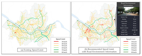
Figure 21.
GIS-based visualization of speed limit information.
By constructing a database of road environment information and linking it with real-time driving speed data, it becomes possible to check speed limit information and road information in the selected area.
If the collection scope of road environment information and real-time data is secured, the GIS visualization of traffic safety information will be facilitated, making it possible to build IVEs in the transportation sector.
Author Contributions
Conceptualization, H.K. and D.J.; methodology, H.K.; software, H.K.; validation, H.K. and D.J.; formal analysis, D.J.; investigation, H.K. and D.J.; resources, H.K.; data curation, D.J.; writing—original draft preparation, H.K.; writing—review and editing, H.K.; visualization, H.K.; supervision, H.K.; project administration, H.K.; funding acquisition, D.J. Both authors have read and agreed to the published version of the manuscript.
Funding
This research was supported by “The 2021 Road Traffic Survey Project” funded by the Ministry of Land, Infrastructure and Transport (MLIT).
Institutional Review Board Statement
Not applicable.
Informed Consent Statement
Not applicable.
Data Availability Statement
The data included in this study are available upon request by contact with the corresponding author.
Conflicts of Interest
The authors declare no conflict of interest.
References
- TAAS, Traffic Accident Analysis System. Available online: http://taas.koroad.co.kr (accessed on 13 January 2021).
- Bauer, R.; Machata, K.; Brandstaetter, C.; Yannis, G.; Laiou, A.; Folla, K. Road Traffic Accidents in European Urban Areas. In Proceedings of the 1st European Road Infrastructure Congress, Leeds, UK, 18–20 October 2016. [Google Scholar]
- Austroads. Guide to Road Safety Part 3: Speed Limits and Speed Management; Austroads: Sydney, Australia, 2008. [Google Scholar]
- International Transport Forum. Road Safety Annual Report; OECD Publishing: Paris, France, 2016; pp. 33–44. [Google Scholar]
- Choi, S.L. A Case of Speed Limits Improvement for Prevention of Traffic Accidents in Japan. Plan. Policy 2014, 4, 100–106. [Google Scholar]
- National Research Council (US). Transport Research Board Special Report 254. In Managing Speed: Review of Current Practice for Setting and Enforcing Speed Limits; National Academy Press: Washington, DC, USA, 1998; pp. 15–138. [Google Scholar]
- WHO. Speed Management: A Road Safety Manual for Decision-Makers and Practitioners; Global Road Safety Partnership: Geneva, Switzerland, 2008; pp. 2–21. [Google Scholar]
- WHO. Global Status Report on Road Safety 2013; WHO Press: Geneva, Switzerland, 2013; pp. 9–13. [Google Scholar]
- WHO. Global Status Report on Road Safety 2015; WHO Press: Geneva, Switzerland, 2015; pp. 11–15. [Google Scholar]
- Forbes, G.J.; Gardner, T.; McGee, H.W.; Srinivasan, R. Methods and Practices for Setting Speed Limits: An Informational Report; United States Federal Highway Administration Office of Safety: Washington, DC, USA, 2012; p. 24.
- Hossseinlou, M.H.; Kheyrabadi, S.A.; Zolfaghari, A. Determining Optimal Speed Limits in Traffic Networks. IATSS Res. 2015, 39, 36–41. [Google Scholar] [CrossRef] [Green Version]
- USLIMITS2: A Tool to Aid Practitioners in Determining Appropriate Speed Limit Recommendations. Available online: http://safety.fhwa.dot.gov/uslimits (accessed on 20 January 2021).
- Cirillo, J.A. Interstate System Accident Research Study II; Interim Report II; Federal Highway Administration: Washington, DC, USA, 1968; Volume 35, pp. 71–75. Available online: https://trid.trb.org/view.aspx?id=107635 (accessed on 21 January 2021).
- Garber, N.J.; Gadirau, R. Speed Variance and Its Influence on Accidents; AAA Foundation for Traffic Safety: Washington, DC, USA, 1988. [Google Scholar]
- Hauer, E. Speed and Safety, Transp. Res Rec. J. Transp. Res. Board 2009, 2103, 11–12. [Google Scholar]
- Parker, M.R., Jr. Effects of Raising and Lowering Speed Limits on Selected Roadway Sections; U.S. Department of Transportation Federal Highway Administration: Washington, DC, USA, 1997.
- Stuster, J.; Coffman, Z. Synthesis of Safety Research Related to Speed and Speed Management; U.S. Department of Transportation Federal Highway Administration: Washington, DC, USA, 1998.
- Fildes, B.N.; Rumbold, G.; Leening, A. Speed Behaviour and Drivers’ Attitude to Speeding; Report No. 16; Monash University Accident Research Centre: Clayton, Australia, 1991; pp. 56–69. [Google Scholar]
- OECD/ECMT. Speed Management; OECD Publishing: Paris, France, 2006; pp. 34–105. [Google Scholar]
- Taylor, M.C.; Lynam, D.A.; Baruya, A. The Effects of Drivers’ Speed on the Frequency of Road Accidents; Transport Research Laboratory Report 421; Transport Research Laboratory: Crowthorne, UK, 2000. [Google Scholar]
- Nilsson, G. Traffic Safety Dimensions and the Power Model to Describe the Effect of Speed on Safety. Ph.D. Thesis, Lund Institute of Technology, Lund, Sweden, 2004. [Google Scholar]
- Elvik, R.; Christensen, P.; Amundsen, A.H. Speed and Road Accidents: An Evaluation of the Power Model; Institute of Transport Economics, Norwegian Centre of Transport Research: Oslo, Norway, 2004. [Google Scholar]
- Elvik, R. The Power Model of the Relationship between Speed and Road Safety: Update and New Analyses; Institute of Transport Economics, Norwegian Centre of Transport Research: Oslo, Norway, 2009. [Google Scholar]
- Elvik, R. A re-parameterisation of the Power Model of the relationship between the speed of traffic and the number of accidents and accident victims. Accid. Anal. Prev. 2013, 50, 854–860. [Google Scholar] [CrossRef] [PubMed] [Green Version]
- Hauer, E.; Bonnesson, J. An Empirical Examination of the Relationship between Speed and Road Accidents based on data by Elvik. In Christensen and Amundsen; NCHRP: Washington, DC, USA, 2006; pp. 17–25. [Google Scholar]
- Chuishi, M.; Xiuwen, Y.; Lu, S.; Jing, G.; Yu, Z. City-wide Traffic Volume Inference with Loop Detector Data and Taxi Trajectories. In Proceedings of the 25th ACM SIGSPATIAL, Redondo Beach, CA, USA, 7–10 November 2017; pp. 1–10. [Google Scholar]
- Samer, R.; Mohamad, K.; Hazem, R. Classification and speed estimation of vehicles via tire detection using single-element piezoelectric sensor. J. Adv. Transp. 2016, 50, 1366–1385. [Google Scholar]
- Lu, J.J.; Park, J.H.; Pernia, J.C.; Disanayake, S. Criteria for Setting Speed Limits in Urban and Suburban Areas in Florida; Florida DOT: Tallahassee, FL, USA, 2003.
- Seoul Metropolitan City. 2015 Seoul Metropolitan City Traffic Monitoring Data. Available online: https://news.seoul.go.kr/traffic/archives/356 (accessed on 7 February 2021).
- Kim, J.O.; Hong, H.D.; Jang, D.I. An Analysis of Error Factors When Traffic Volume Predicted with Navigation Loaded Vehicles. In Spring Conference of the Korean Transportation Association; Korea Society of Transportation: Seoul, Korea, 2016. [Google Scholar]
- Doo, C.U.; Kim, H.S.; Kim, K.H.; Lee, S.B.; Jo, H.J. Traffic Safety Engineering; Chung Moon Gak: Seoul, Korea, 2013; pp. 163–167. [Google Scholar]
- California Department of Transportation. California Manual for Setting Speed Limits; California Department of Transportation: Sacramento, CA, USA, 2014; pp. 13–18.
- Jeong, H.J.; Yoeun, J.S.; Bae, S.H. Prediction of Main Road Traffic Conditions with Prove Vehicle for a Basis in Urban Road. In Spring Conference of the Korean Transportation Association; Korea Society of Transportation: Seoul, Korea, 2016. [Google Scholar]
- Shinar, D. Traffic Safety and Human Behavior, 1st ed.; Emerald Group Publishing Ltd.: Bingley, UK, 2007; pp. 274–281. [Google Scholar]
- Warren, D.; Xu, G.; Srinivasan, R. Setting Speed Limits for Safety. Public Roads 2014, 77. Available online: https://www.fhwa.dot.gov/publications/publicroads/13sepoct/02.cfm (accessed on 7 February 2021).
- Srinivasan, R.; Parker, M.; Harkey, D.; Tharpe, D.; Sumner, R. Expert System for Recommending Speed Limits in Speed Zones Final Report; Transportation Research Board: Washington, DC, USA, 2006; pp. 39–42. [Google Scholar]
- Elvik, R. Assessing Causality in Multivariate Accident Models. Accid. Anal. Prev. 2011, 43, 253–264. [Google Scholar] [CrossRef] [PubMed]
- Ichinose, T.; Shimodozono, K.; Hanaki, K. Impact of anthropogenic heat on urban climate in Tokyo. Atmos. Environ. 1999, 33, 3897–3909. [Google Scholar] [CrossRef]
- Teofel, B.; Sushama, L.; Poitras, V.; Dukhan, T.; Belair, S.; Moreno, L.M.; Sun, L.; Pasmito, A.P.; Bitsyamlak, G. Impact of COVID-19-Related Traffic Slowdown on Urban Heat Characteristics. Atmosphere 2021, 12, 243. [Google Scholar] [CrossRef]
- Edler, D.; Kühne, O.; Keil, J.; Dickmann, D. Audiovisual Cartography: Established and New Multimedia Approaches to Represent Soundscapes. KN J. Cartogr. Geogr. Inf. 2019, 69, 5–17. [Google Scholar] [CrossRef] [Green Version]
- Feldstein, I.T.; Dyszak, G.N. Road crossing decisions in real and virtual environments: A comparative study on simulator validity. Accid. Anal. Prev. 2020, 137, 105356. [Google Scholar] [CrossRef] [PubMed]
- Sobhani, A.; Farooq, B. Impact of smartphone distraction on pedestrians’ crossing behaviour: An application of head-mounted immersive virtual reality. Transp. Res. Part F Traffic Psychol. Behav. 2018, 58, 228–241. [Google Scholar] [CrossRef] [Green Version]
- Nazemi, M.; Eggermond, M.A.B.V.; Erath, A.; Schaffner, D.; Joos, M.; Axhausen, K.W. Studying bicyclists’ perceived level of safety using a bicycle simulator combined with immersive virtual reality. Accid. Anal. Prev. 2021, 151, 105943. [Google Scholar] [CrossRef] [PubMed]
Publisher’s Note: MDPI stays neutral with regard to jurisdictional claims in published maps and institutional affiliations. |
© 2021 by the authors. Licensee MDPI, Basel, Switzerland. This article is an open access article distributed under the terms and conditions of the Creative Commons Attribution (CC BY) license (https://creativecommons.org/licenses/by/4.0/).