Novel Data-Driven Models Applied to Short-Term Electric Load Forecasting

Abstract

This work brings together and applies a large representation of the most novel forecasting techniques, with origins and applications in other fields, to the short-term electric load forecasting problem. We present a comparison study between different classic machine learning and deep learning techniques and recent methods for data-driven analysis of dynamical models (dynamic mode decomposition) and deep learning ensemble models applied to short-term load forecasting. This work explores the influence of critical parameters when performing time-series forecasting, such as rolling window length, k-step ahead forecast length, and number/nature of features used to characterize the information used as predictors. The deep learning architectures considered include 1D/2D convolutional and recurrent neural networks and their combination, Seq2seq with and without attention mechanisms, and recent ensemble models based on gradient boosting principles. Three groups of models stand out from the rest according to the forecast scenario: (a) deep learning ensemble models for average results, (b) simple linear regression and Seq2seq models for very short-term forecasts, and (c) combinations of convolutional/recurrent models and deep learning ensemble models for longer-term forecasts.

1. Introduction

Short-term load forecasting (STLF) is of vital importance to utility companies in many areas, such as maintenance, operations, and reliability. Achieving accurate load forecasts is a difficult task due to the highly non-linear nature of the underlying model. Forecasts in this area have been historically treated with time-series statistical analysis methods, e.g., autoregressive integrated moving average (ARIMA) [1], with a clear trend towards the use of machine learning techniques in current times [2].

STLF is a solid area of research with a significant body of literature exploring the application of specific techniques to specific datasets or the review of techniques applied in different research works to different datasets. Meanwhile, the number of papers proposing new forecasting methods in the areas of dynamic modeling and machine learning (and more specifically deep learning) continues to grow, which makes it very interesting to have a systematic comparison, based on a single dataset, of a significant number of novel techniques.

In this work, we propose a comprehensive study of STLF with a significant number of data-driven forecasting models that are novel or rarely applied to STLF, such as: (a) dynamic mode decomposition (DMD) [3,4,5], (b) deep learning (DL) models based on specific combinations of convolutional neural networks (CNN) and recurrent neural networks (RNN) [6,7], (c) sequence to sequence (Seq2seq) models with and without soft attention [8,9,10], and (d) deep learning ensemble models specially targeted for time-series forecasting [11]; and a set of well-known forecasting models, such as: (e) classic machine learning (ML) models: linear regression, random forest, gradient boosting, k-nearest neighbors, support vector regression and AdaBoost [12,13,14,15], (f) multi-layer perceptron [2], and (g) deep learning models based on separate CNN and RNN networks [13,14]. By jointly evaluating the novel or less used techniques with the best known, we can compare their performance in different scenarios.

We carried out the study by applying the different models to a real dataset of power consumption from a Spanish utility for the province capital of Soria (Spain). This dataset has been extensively studied previously [16,17,18,19,20,21,22,23].

This work is different from other studies: (a) by applicability, not being a reference to other studies and applying all the models to the same dataset which allows comparison of results, (b) by novelty, by including, in the same study, the results from DMD [5], new DL ensemble models based on gradient boosting principles [11], specific configurations of CNN/RNN [6,7], and Seq2seq models [8,9,10], and (c) by extension, by considering a large number of different models under different scenarios.

STLF needs a previous preparation of the load values used as predictors. The preparation consists of aggregating these values in discrete time intervals (time-slots) that can be seconds, minutes, or hours, and the forecast can be based on a different number of previous values (predictors) that are obtained with a rolling window process applied to the past values. The length of the rolling window defines the number of predictors. With these predictors, the forecast can be extended to the following time-slot or to several time-ahead time-slots (k-step ahead forecast). Finally, the value of the predictors can be a scalar (load value), or a vector composed of the load value plus additional information, such as date/time or weather data. Considering the scenario with vector predictors and multiple time-ahead forecasts, we arrive at a challenging multivariate multi-output regression problem. The influence of these parameters: (a) length of rolling window, (b) length of time-ahead forecast, and (c) features used to form the predictors, is analyzed in this research in combination with the different natures exposed by the models.

Time-series statistical analysis algorithms (e.g., ARIMA) have not been contemplated as they are trained to specific past values, while our goal is to have a single algorithm that can be trained once and generalizes to new past values. In addition, they are mainly intended for single-output forecasts and their extension to multi-output scenarios (i.e., forecasting $k$ future values) generates complex models (e.g., VARIMA).

To appraise different possible evaluation objectives associated with STLF, we have obtained six different metrics to assess the forecasting performance of the models: mean square error (MSE), mean absolute error (MAE), median absolute error (MAD), coefficient of determination ($R^2$), relative root mean squared error (RRMSE), and symmetric mean absolute percentage error (sMAPE). We also analyze the influence of the time-ahead forecast interval and the rolling window length on these metrics.

Results are presented following three different forecast objectives: very short-term forecasts (immediate time-slots in the forecast time horizon), longer-term forecasts (last time-slots in the forecast time horizon), and forecast average (average of all time-slots in the forecast time horizon). Considering these three scenarios, we have obtained the three best groups of models according to the different forecast objectives: (a) deep learning ensemble models for average results, (b) simple linear regression and Seq2seq models for very short-term forecasts, and (c) combinations of convolutional/recurrent models and deep learning ensemble models for longer-term forecasts.

We have explored the use of deep learning blocks based on the ensemble model presented in [11], called gaNet. The gaNet architecture has been used for IoT traffic prediction [11] and classification [24]. This is the first time that this architecture has been applied to STLF. A gaNet architecture is made up of small deep learning networks formed by a few Convolutional (Conv) and/or RNN layers. These networks are organized as repeating blocks whose outputs are combined (after an aggregation function) into a final output. The input to the architecture is shared by all the blocks. This architecture is connected to gradient boosting models, stacked models [25], and residual networks [26].

It is worth noting the excellent results of the proposed deep learning ensemble model (gaNet) and how it excels in average results and in longer-term (most difficult) forecasts. This good behavior can be connected with having a repeating set of randomly initialized deep learning blocks, in line with other studies that connect the importance of a rich set of random initializations with the behavior of deep learning models [27]. Deep ensembles can also provide an improvement in uncertainty estimates for samples outside the expected data distribution, through appropriate data selection and a specific loss function that maximizes model diversity [28]. This work contributes to provide additional results that confirm the good behavior of deep ensembles under an additional perspective provided by gaNet. In previous works [11,24], gaNet has been applied to time-series forecasts with a panel data structure (a list of entities, each with an associated time-series), whereas this work applies it to a single time-series with different requirements for data preparation and the validation/testing process.

An additional objective of the study is to put forward the availability of accurate forecast results as a valuable tool for identifying new applications, such as: (a) identification of anomalous consumption patterns due to excessive deviations from the forecasts, which can be used as alarms for security or fraud situations and, (b) simulation of what-if non-standard load scenarios and their consequences. These two applications are important for smart grids and their convergence with the IoT (Internet of Things) infrastructure with higher cybersecurity and fraud risks [29,30].

As a summary, the contributions of this work are: (1) Extend an ensemble deep learning model (i.e., gaNet) based on the gradient boosting architecture to the particular needs of STLF. (2) Present a thorough analysis of STLF models with a special emphasis on novel methods, e.g., gaNet, DMD, Seq2seq, and combinations of CNN/RNN models. (3) Apply all the models to a previously well-studied dataset of real electricity consumption, allowing comparisons to be made on a single dataset in a homogeneous and structured way, which allows comparison of results and drawing conclusions on common bases. (4) Analyze the impact on forecasts due to: (a) length of rolling window, (b) length of time-ahead forecast, and (c) features used to form the predictors. (5) Present the best groups of models according to different forecast objectives. (6) Apply to STLF, for the first time, as far as we know, the gaNet model and the specific configurations that combine convolutional and recurrent layers as proposed here [6,7].

The organization of the paper is as follows: Section 2 summarizes related works. Section 3 describes the dataset and the forecast models. Section 4 provides the results and Section 5 presents the conclusions.

2. Related Works

There is a large body of recent work on STLF applying many different techniques which show that even when it may be seen as a well-known area of study, it is still an important area of research due to its technical difficulty and economic impact of having an accurate load forecast. The intention of this work is to contribute to this area by providing practical results on the application of some of the newest methods for time-series forecasting applied to STFL in an extensive and homogeneous way.

We will present related works considering the applied methods, global review studies, and some of the anticipated applications that result from having accurate forecasts. The presentation will focus more on adopted methods and processes than on performance metric comparison, since the diversity of datasets, the difference in load magnitudes, the differences in the implementation of the metrics, and the various test/validation procedures make it very difficult to perform a homogeneous comparison of results.

Review of current techniques: The work in [2] presents a comprehensive review of the techniques used to forecast electricity demand, analyzing the different types of forecasts, parameters affected, and techniques used, together with a literature review and a taxonomy of the main variables involved in the problem. The work in [13] presents a detailed review of recent literature and techniques applied for building energy consumption modeling and forecasting.

A complete review of machine learning for load prediction is given in [31] with emphasis on the following methods: tree-based methods and random forest, support vector regression (SVR), neural networks, ensemble learning, statistical methods (ARMA, ARIMA,…), gaussian processes, k-nearest neighbors regressor (KNN), and fuzzy time-series algorithms. An alternative review is given in [32] highlighting the following models: linear regression, artificial neural networks (ANN), SVR, statistical methods, restricted Boltzmann machine, and deep learning (CNN and LSTM). A recent review of machine learning models applied to load forecasting focusing on performance metrics results is proposed in [33]. This study presented the following methods as the most frequently implemented in electric power forecasting: statistical methods, artificial neural networks (ANNs), support vector machines (SVMs), decision trees (DTs), adaptive neuro fuzzy inference systems (ANFISs), and recurrent neural networks (RNNs).

The work in [34] presents the application of five machine learning models for STLF: multiple linear regression, KNN, SVR, and gradient boosting. The best performance is obtained for gradient boosting. Authors in [35] present a recent and systematic review of techniques applied to load forecasting with an emphasis on neural networks and hybrid models. The main models presented are: SVM, GBM, random forest (RF), KNN, neural networks, decision trees, statistical methods, CNN, LSTM, and the adaptive neuro-fuzzy inference system (ANFIS). The authors in [36,37] provide an study of methods to use in load forecasting considering different forecasting problems and objectives. The main methods discussed are: statistical methods, AdaBoost, GBM, random forest, generalized additive models (GAM), gaussian processes, KNN, linear regression, and support vector regression. The work in [38] presents an extensive literature review with no mention of dynamical systems modeling or deep learning or ensemble deep learning models. The methods mentioned are: multioutput linear regression, generalized additive models, statistical models, neural networks, support vector machines, gradient boosting, and fuzzy regression. The review in [39] favors the use of artificial neural networks, support vector regression, and fuzzy logic models.

Dynamical systems modeling: There is a growing current interest in the application of dynamical systems analysis tools based on reduced-order models and, in particular, in the use of dynamic mode decomposition to STLF. The work in [5] provides a DMD study applied to electric load data from a utility operator in Queensland, Australia. In this work, the DMD algorithm presents better forecasting results than classic time-series autoregressive approaches. They offer a one day ahead forecast based on the load values of the previous 4 days, presenting a MAPE result of 2.13. A similar application of DMD is carried out in [40] but applying DMD to predict forecast errors followed by an extreme value constraint method to further correct the forecasts. The algorithm is applied to actual load demand data from the grid in Tianjin, China, and the results obtained with DMD are compared with a series of additional techniques (autoregressive moving average, neural networks, support vector machines, extreme learning machines, etc.). According to the authors, the proposed method shows greater accuracy and stability than alternative ones, with a best average root mean squared error (RMSE) of 476.17. In [41], the authors employ an empirical mode decomposition technique to extract different modes from the load signal, and apply an independent deep belief network for each mode prediction, with a subsequent aggregation of results (ensemble) to obtain the final load forecast. More classic ensemble techniques for forecasting electricity consumption in office buildings are investigated in [42], comparing gradient tree boosting (GTB), random forests (RF), and a specifically adapted AdaBoost model that presents the best results.

Classic machine learning: A substantial number of works have presented several classic machine learning models to STLF. A feed-forward artificial neural network (FF-ANN) is used in [43] to forecast the electricity consumption for residential buildings for 24 h. The results are compared with other models including GTB and RF, selecting the best model at each forecast iteration. The best average result for the different test iterations is obtained for the ANN with an RMSE of 2.48. The work in [44] presented a theoretical review of the most commonly used ML methods for STLF, including ANN and a support vector for regression. The work in [45] presents an interesting pipeline method based on combining a feature transformation using a clustering approach followed by a support vector regression. The authors in [46] introduce an additive regression model for STLF.

Statistical analysis methods: Time-series statistical analysis models for STLF are discussed in detail in [1] with forecasts at an hourly interval applied to load data from the Electric Reliability Council of Texas (ERCOT). They present results applying ARIMA and Seasonal Autoregressive Integrated Moving Average (SARIMA) models achieving an average mean absolute percentage error (MAPE) between 4.36% to 12.41%.

Sequence to sequence models: The sequence to sequence (Seq2seq) architecture that originated in the field of natural language processing (NLP) has been applied in recent works to STLF. The authors in [47] apply different Seq2seq architectures, comparing them with other DL models based on recurrent and convolutional layers. The models are applied to two different datasets (scenarios): one for an individual household electric power consumption data set (IHEPC) located in Sceaux, France, and the other for the GEFCom2014 public dataset made available for the global energy forecasting competition 2014. The best results (RMSE between 17.2 and 0.75 depending on the scenario) are obtained with convolutional and recurrent architectures together with deep neural networks with dense layers. Considering average results, the Seq2seq models do not provide the best results. The conclusions obtained in this work are consistent with the results obtained by the present study. A similar study is presented in [48], where research was conducted comparing a Seq2seq model (with and without attention) with alternative DL models based exclusively on different types of recurrent networks, such as long short-term memory network (LSTM) and gated recurrent unit (GRU). In this case, the Seq2seq model presents the best results for short-term forecasting, also in accordance with the results obtained in the present work. A generic Seq2seq with a specific attention mechanism is proposed in [49] for multivariate time-series forecasting.

Deep learning models: Using the same dataset proposed for this work, [16] presents an ANN model that works on a 24 h day-ahead forecasting of electric loads previously aggregated into clusters by consumption patterns. The patterns are obtained with a self-organizing map (SOM) followed by a k-means clustering algorithm. The work in [50] introduces a deep learning architecture based on an ensemble of convolutional blocks acting on segregated subsets of the input data. The model is applied for day-ahead forecasting of individual residential loads with data obtained from a smart metering electricity customer behavior trial (CBTs) in Ireland. The work focuses on achieving low training time and high accuracy, the proposed model being the best in both aspects with an MAE of 0.3469. The authors in [51] present a simple MLP regressor with a sophisticated selection of features based on previous consumptions and weather data. The work in [52] introduces a combined model of CNN and LSTM layers for STLF. A comparison between recurrent neural networks (LSTM) and support vector regression (SVR) is provided in [53], showing that the bidirectional LSTM model outperforms both the unidirectional LSTM and the SVR models.

3. Materials and Methods

This section presents the dataset and forecast models (Section 3.1 and Section 3.2, respectively) used for the experiments.

3.1. Selected Dataset

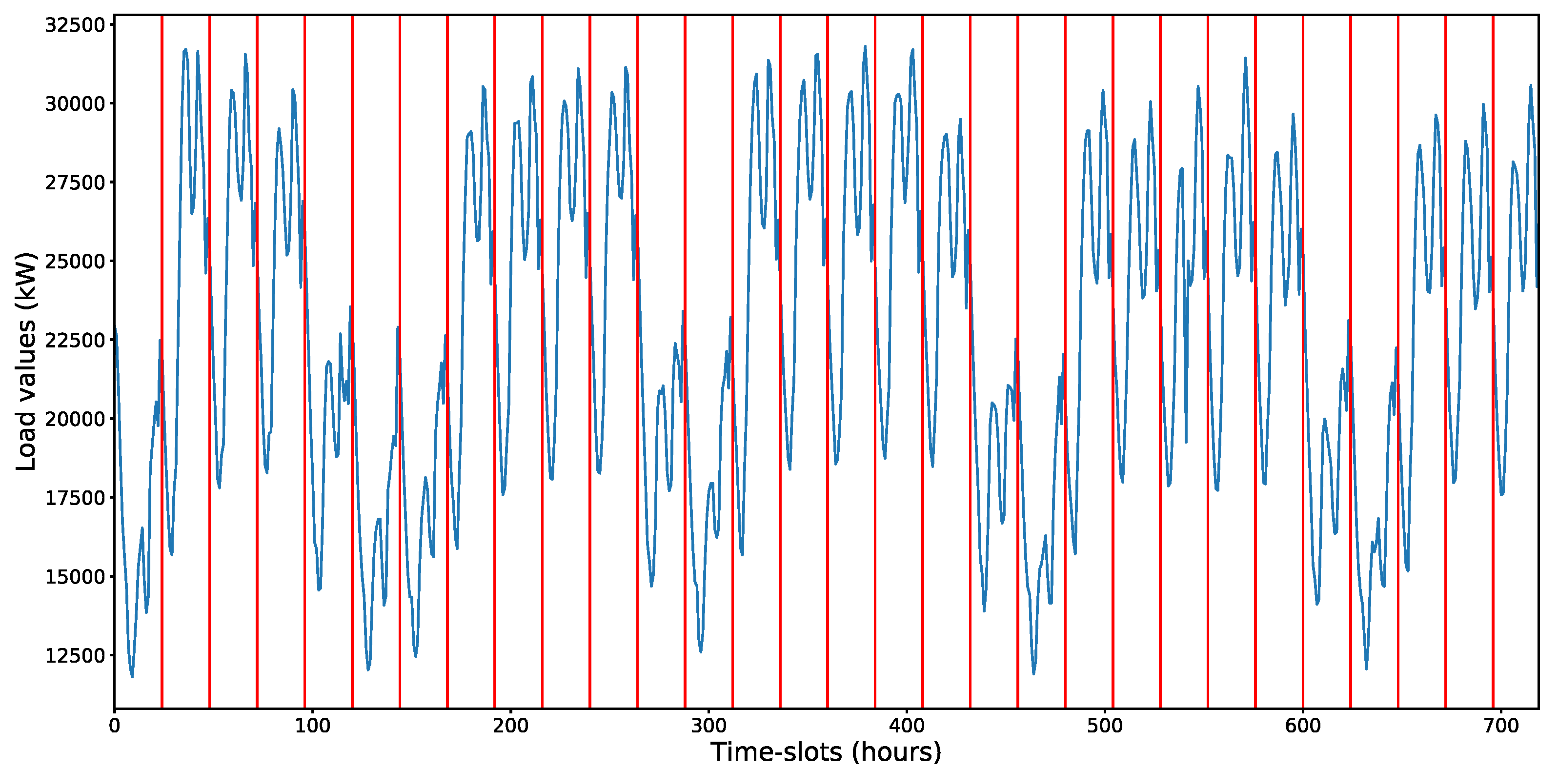
The dataset employed in this research corresponds to real data from a Spanish utility over a period of three years. The load distribution presents similarities to that of a microgrid [16], with a value range between 7370 and 39,550 kW. The values have annual periodicity, also with strongly defined daily and weekly periodicity (Figure 1).

Figure 1. Chart showing the load values for a period of 30 days and time-slots of 1 h. The vertical red lines indicate a 24 h period (1 day). We can observe the strong daily and weekly periodicity.

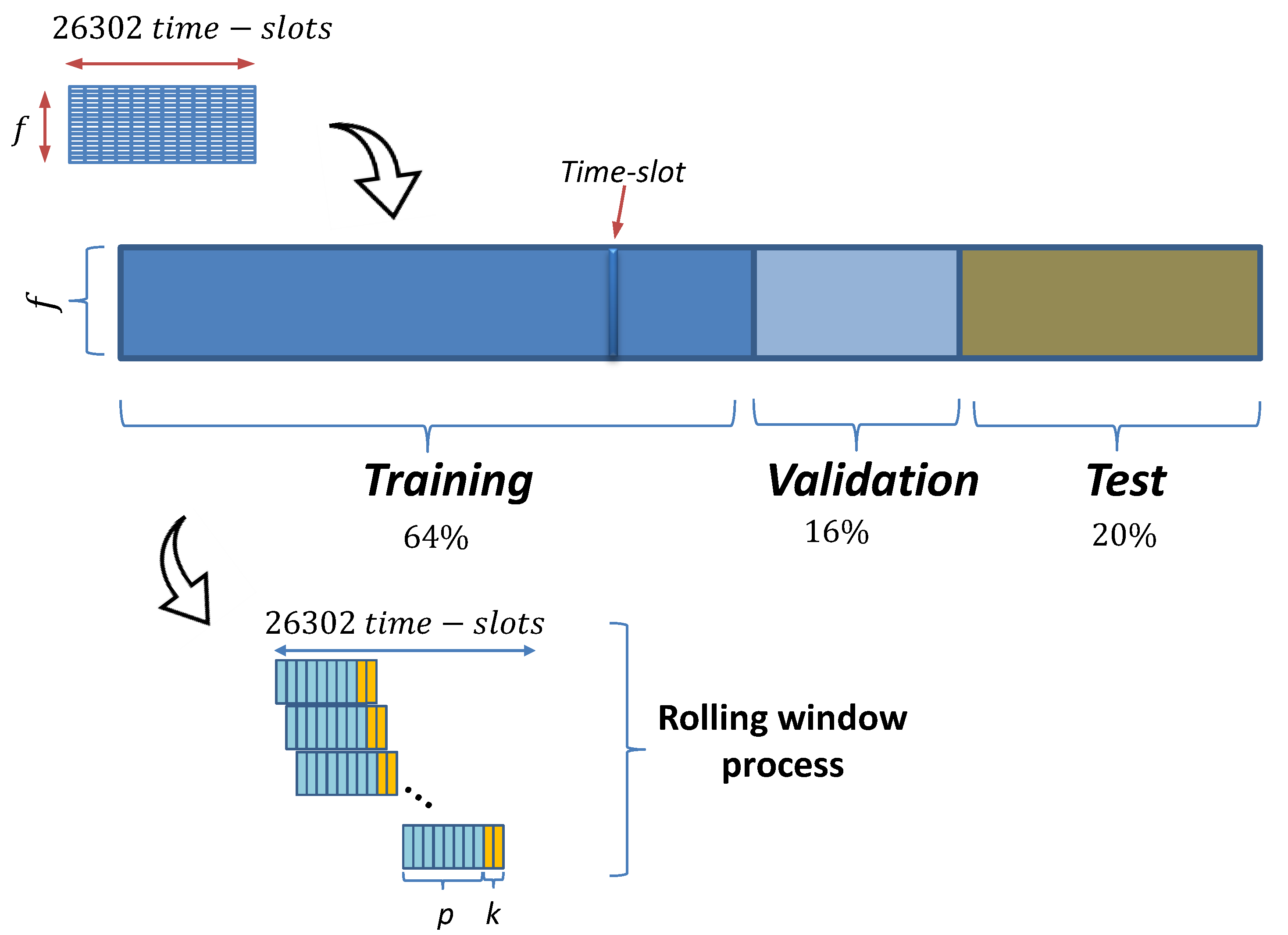
Load values were aggregated in time-slots of one hour. The total number of time-slots corresponded to 26,302 h. Additional exogenous features were also considered: (a) Date/time features: month, time, day of the week, and weekend indicator. (b) Weather features: mean and standard deviations for the atmospheric pressure, wind speed, wind direction (degrees), humidity, and solar radiation. Continuous features were scaled in the range [0,1]. Categorical features were one-hot-encoded. We considered four different sets of features out of the many possible feature combinations: (a) 1 feature: electricity load, (b) 45 features: date/time (day of week, weekend, hour, month) and load, (c) 57 features: date/time, weather and load, and (d) 76 features: date/time, load, plus day of the month (one-hot-encoded). The number of features for the different feature sets is denoted by $f$ (Figure 2). The weather and day of the month features did not provide a clear improvement in the forecast metrics.

Figure 2. Division of the original dataset into training, validation, and test sets with a data proportion of 64, 16, and 20%, respectively. A rolling window process was used to extract the predictors sequence ($p$ time-slots used as predictors) and the real time-ahead load values ($k$ time-ahead forecast length). Each time-slot is represented by a vector of predictors with $f$ components (load value, date/time features, etc.).

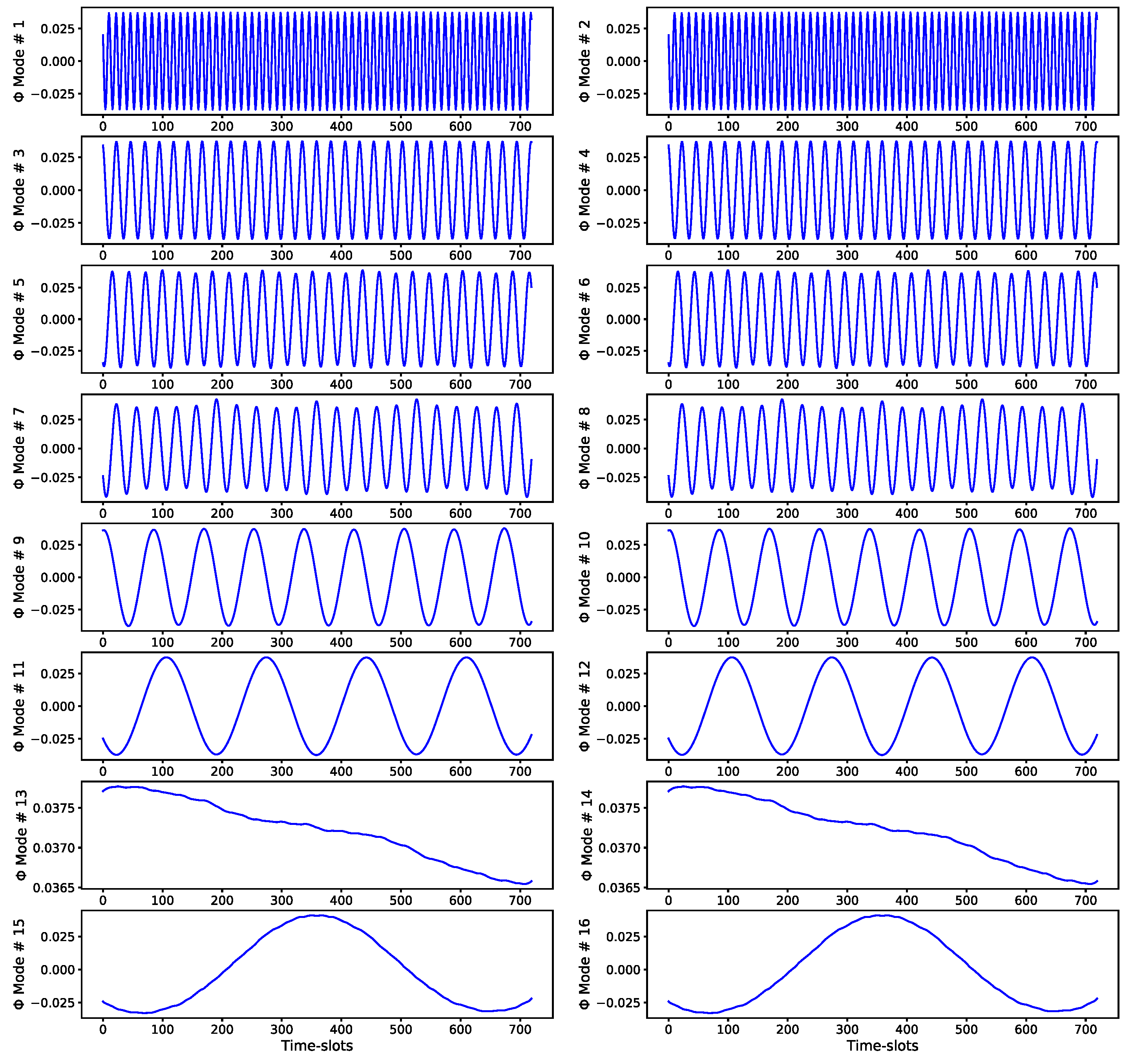
Figure 2 presents how the original dataset was divided into training, validation, and test sets with a data proportion of 64, 16, and 20%, respectively. Figure 2 also presents the rolling window process used to extract the predictors sequence ($p$ time-slots used as predictors) and the real time-ahead values ($k$ time-ahead forecast length). The validation data were used to assess model performance during training. The test set was used to provide all final results in Section 4. As a summary, we consider the following ranges of values for the parameters $p$, k, and $f$: (a) $p$: 24 (using the previous day of data—24 h), 168 (previous week of data—168 h), or 720 (previous month of data—720 h); (b) k: 24 (1-day forecast horizon), 168 (1-week horizon), or 720 (1-month horizon); and (c) $f$: 1, 45, or 57. The forecast results for different combination for these values ($f, p, k$) are reported separately in Section 4 and the Appendix A.

3.2. Models Description

This section presents the different models used in our research. The models have been grouped according to their characteristics. The presentation of results in Section 4 will follow the groups described here. The groups were the following:

-

Classic machine learning models: We considered the following models: linear regression, random forest, gradient boosting, k-nearest neighbors, support vector regression, and AdaBoost. These models provide a good selection of machine learning models widely applied to STLF.

-

Deep learning models: As already mentioned, deep learning models are currently the main trend in STLF. We applied various configurations of convolutional neural networks (CNN) and long short-term memory (LSTM) networks, a type of recurrent neural networks (RNN). The combination of CNN and LSTM networks has provided some of the best results, in accordance with the results obtained in other works applying the same configurations in other fields (network traffic analysis, video quality of experience, etc.) [6,7].

-

Deep learning ensemble models: It is well-known that aggregating the capabilities of various estimators can increase their effectiveness in reducing errors and avoiding overfitting. There are several aggregation strategies, and boosting is one of the most important and provides state-of-the-art estimators. Bringing together boosting and deep learning has shown very good results in other forecasting problems [11]. The DL ensemble models included in this work follow the gaNet architecture [11], which is a deep learning boosting ensemble model specifically intended for time-series forecasting.

-

Seq2seq models: The sequence to sequence model had its origins in the field of NLP, but it has been extended to many time-series prediction problems. It has rarely been used in STLF even when it provides good results when applied [48].

-

Dynamic mode decomposition (DMD) models: These models attempt to approximate the non-linear latent drivers of a system by a linear transformation [4]. They are mainly applied in finance and fluid dynamics for both prediction and characterization of system behavior [3,54]. These models provide important information about the principal modes of the signal and their behavior. DMD is a technique that is currently attracting interest in STLF [5,55].

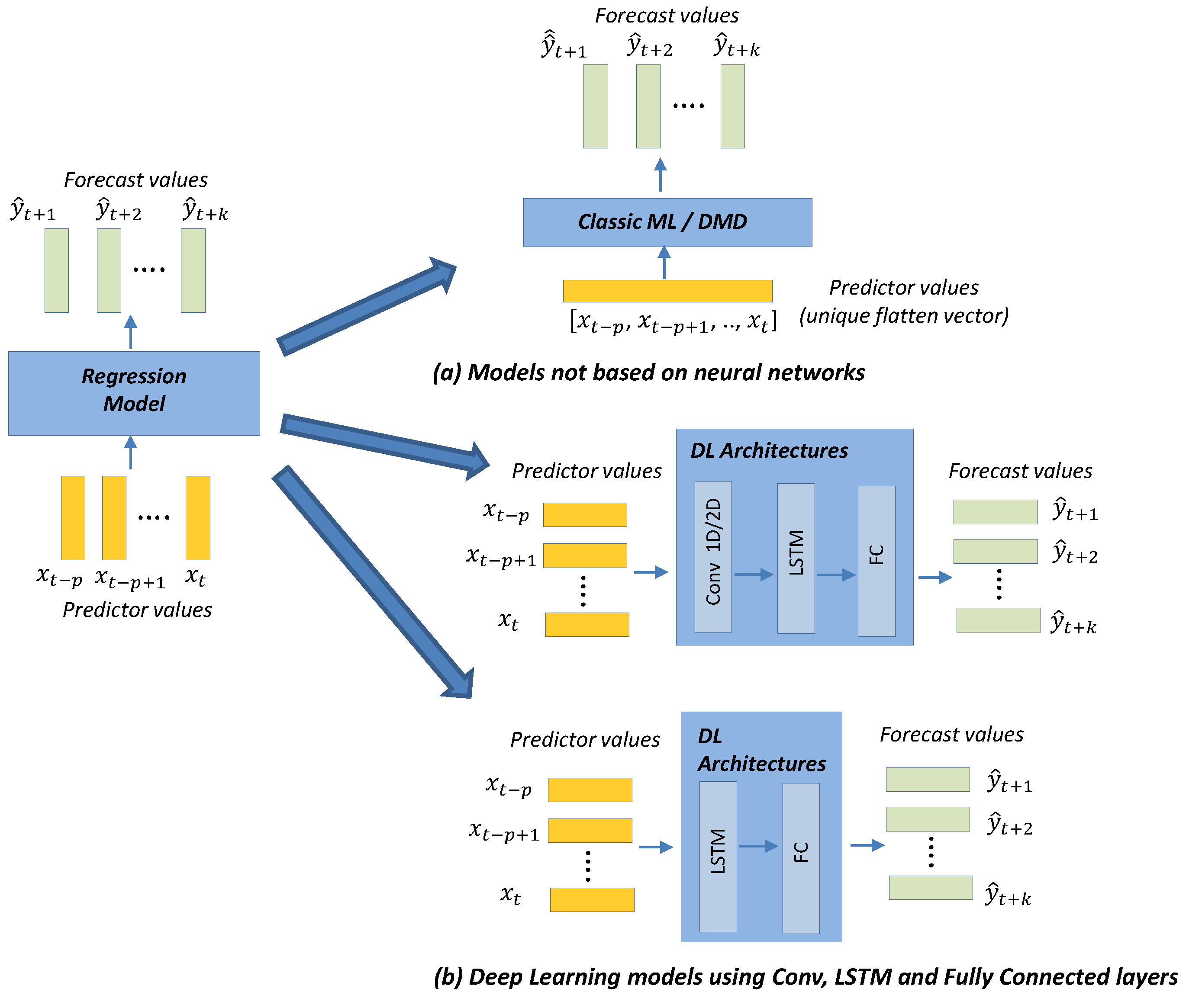
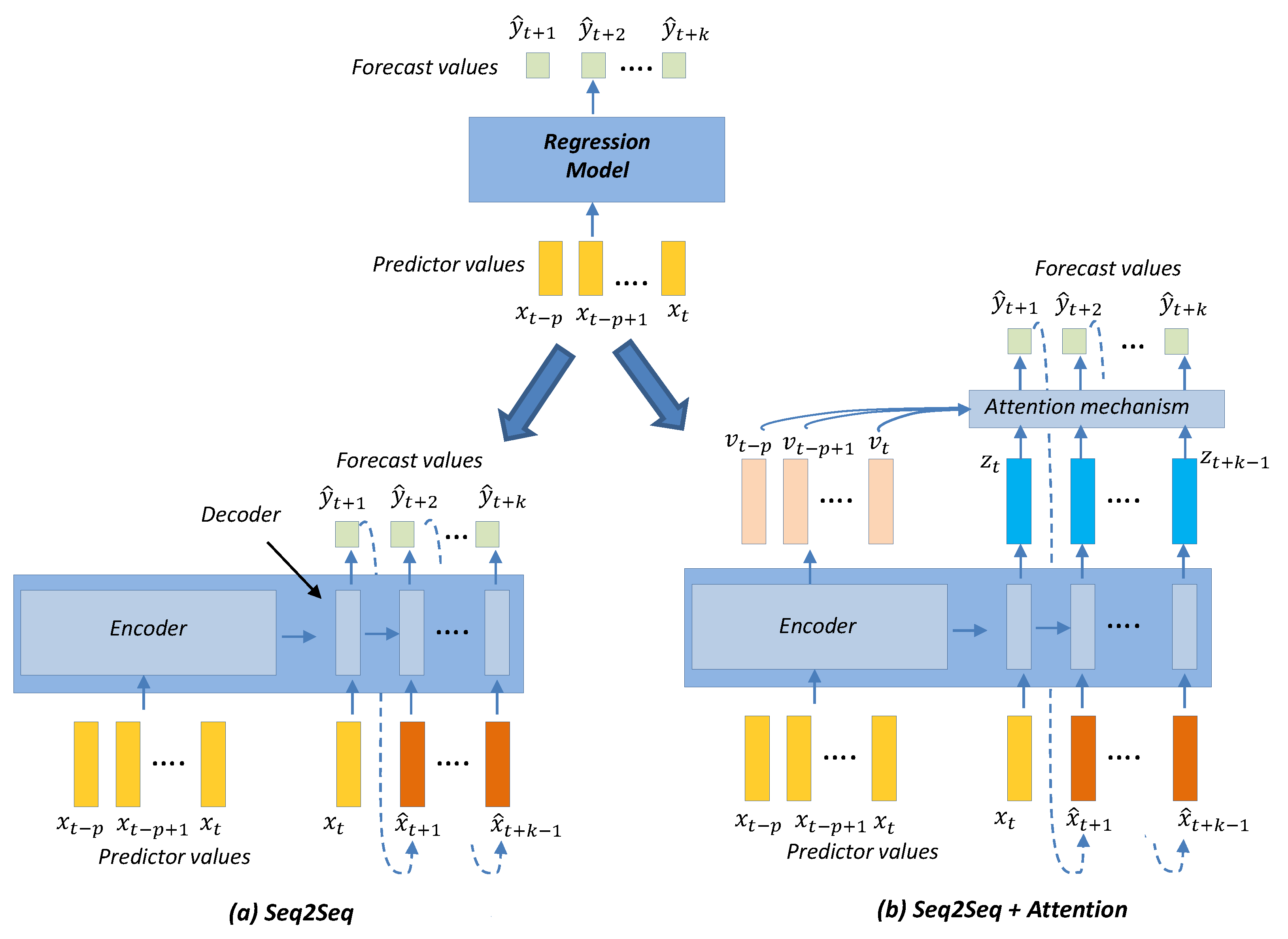
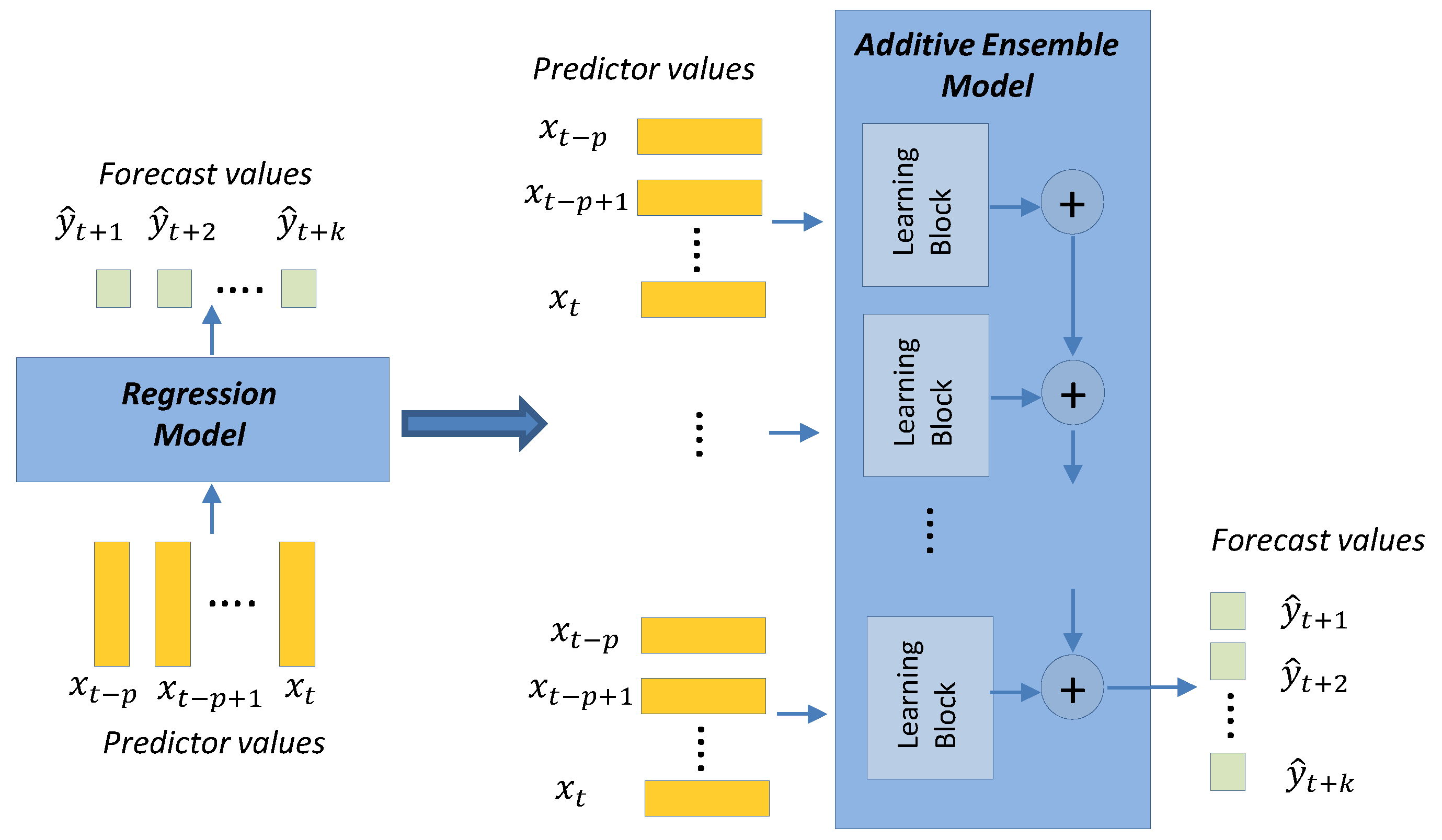
Figure 3, Figure 4 and Figure 5 show different instances of the generic regression algorithm needed to transform the input sequence of $p$ predictors into the output forecast sequence of length $k$. Figure 3 presents details of the models: classic ML, dynamic mode decomposition (DMD) and DL architectures. Figure 4 presents the details for the Seq2seq model with and without attention. Figure 5 presents the details for the ensemble models based on the gaNet architecture [11], which are deep learning ensemble configurations based on gradient boosting principles and are particularly suitable for time-series forecasting. These were the ensemble models used in this work.

Figure 3. Detail of the models: classic ML, dynamic mode decomposition (DMD), and DL architectures.

Figure 4. Detail of the Seq2seq and Seq2seq + attention models.

Figure 5. Detail of the deep learning ensemble models used in this work.

Figure 3 presents a schematic view of the ML, DL, and DMD models with an emphasis on showing the inputs received by the models and the generated outputs. We can observe how the inputs for the ML and DMD models are different to the inputs for the DL models, the reason being that DL models can receive vector-valued inputs, i.e., both LSTM [48] and 1D/2D CNN [47] models can receive a vector-valued sequence (with length p) where each timestep is represented by a vector of values. However, the ML and DMD models expect a sequence of scalar values (longitudinal data) as input; the way to transform the input data for these models is to flatten the vectors over all time-steps.

The DMD model [3,4] is different from the rest of the models since it has its origin in the study of dynamical systems, exploring the construction of a linear approximation to the dynamics of the system. It is a data-driven method based on approximating the temporal evolution of the system by a linear transformation given by a matrix ($A$). The eigenvectors and eigenvalues of this matrix define the dynamic modes of the system and their temporal evolution. The matrix $A$ that defines the mapping between past ($x_t$) and future ($x_{t+1}$) snapshots of the system follows Equation (1). This expression can be extended to a complete set of snapshots obtained using the rolling window method presented in Figure 2. The snapshots set can be arranged in a matrix $X\in {ℝ}^{p\times N}$, where p is the length of the snapshots and $N$ is the number of snapshots obtained with the rolling window process. Likewise, a new matrix $\widehat{X}$ is created by selecting the same columns of $X$ with a lag, i.e., if ${\widehat{X}}_i$ is the $i$column of matrix $\widehat{X}$, then ${\widehat{X}}_i=X_{i+1}$. Once $X$ and $\widehat{X}$ are defined, we obtain Equations (2) and (3), where $X^{†}$ is the pseudo inverse of $X$. The eigenvectors of $X$ define the dynamic modes of the system. The problem with Equation (3) is that the matrices involved are large and their computation is difficult. The DMD method provides a solution to obtain the eigenvectors of $A$ by computing the singular value decomposition of $X$ (Equation (4)) and the matrix $\tilde{A}$ (Equation (5)). The matrix $\tilde{A}$ can be considered as the linear best fit for our original system. The matrix $\tilde{A}$ has a much lower dimensionality than $A$, which allows us to easily obtain its eigenvalues ($\mathsf{\Lambda }$) and eigenvectors ($W$) (Equation (6)). Finally, the eigenvalues of $A$ are the same as the eigenvalues of $\tilde{A}$ [3] and the eigenvectors of $A$ (denoted as $\mathsf{\Phi }$) can be obtained from the previously obtained elements and computed following Equation (7).

$$x_{t+1}=A x_t$$

(1)

$$\widehat{X}=A X$$

(2)

$$A=\widehat{X} X^{†}$$

(3)

$$X=U\mathsf{\Sigma }{V}^{*} ; \widehat{X}=AU\mathsf{\Sigma }{V}^{*}$$

(4)

$$U^{*}\widehat{X} V{\mathsf{\Sigma }}^{-1}=U^{*}AU=\tilde{A}$$

(5)

$$\tilde{A}W=W\mathsf{\Lambda }$$

(6)

$$\mathsf{\Phi }=\widehat{X} V{\mathsf{\Sigma }}^{-1}\mathrm{W}$$

(7)

The previous presentation of DMD corresponds to a complete deployment of the algorithm. To further reduce computational needs, we can keep just the leading eigenvalues ($\mathsf{\Lambda }$) and eigenvectors ($W$) of $\tilde{A}$while preserving most of the decomposition energy [3,4]. In this way, we reduce the dynamics of the system to its main eigenvalues and its corresponding eigenvectors ($\mathsf{\Phi }$). In Section 4, we present the main eigenvectors of the DMD decomposition for our data set for different rolling window lengths ($p$).

DMD allows us to implement forecasts [3,4] using Equation (8), where $x_t$ is a forecast for time t, ${\mathsf{\Lambda }}^t$ is the power t of the diagonal matrix $\mathsf{\Lambda },$ which is easily computed, and $b_0$ is an initial condition obtained by multiplying the inverse of the matrix $\mathsf{\Phi }$ with the initial snapshot (first column) ($X_0$) of the matrix $X$:

$$b_0={\mathsf{\Phi }}^{-1} X_0; x_t={\mathsf{\Phi }\mathsf{\Lambda }}^t{b}_0$$

(8)

As shown in Section 4, the DMD algorithm is not particularly efficient at forecasting, but it is very useful for identifying the fundamental modes and temporal behavior of a time series.

The classic ML models with best combined performance results, considering both the forecasting metrics and execution times, are: linear regression (LR) and random forest (RF) [13]. They are well-known ML models. They are robust, fast and do not require intensive hyperparameter tuning and are good at preventing overfitting. These models are particularly interesting for very short-term forecasts (Section 4). However, they experience problems with large values of the parameters $p$ and $f$ that produce large input vectors, since the inputs of these models are the predictors arranged as a flat vector. This has an impact on memory problems and computational times. Furthermore, these models allow a single prediction output, thus requiring as many regressors as outputs with a significant impact on training times for multi-step ahead forecasts, as is our case.

The DL models considered follow two configurations, depicted in Figure 3: (a) recurrent networks formed by one LSTM layer or two stacked LSTM layers plus a fully connected (FC) final layer, or (b) networks formed by a combination of 1D-Convolutional (1D-Conv) layers (between one to three) followed by one or two LSTM layers and a final FC layer. These two configurations have shown very good classification and regression performance in other fields [6,7], as well as other time-series forecasting problems [11]. We also explored the use of 2D-Conv layers instead of the 1D-Conv (common for time-series) layers by transforming the input sequence of vectors into a matrix that is interpreted as a pseudo-image, following the approach in [7]. Contrary to the good performance of this approach in other fields, in this case the results obtained by the architecture 2D-CNN + LSTM were not as good as expected (Figure A1—Appendix A).

The number of epochs used for training all models was 100, with an early-stop criteria established in 10 epochs without improvements. The batch size was 20 samples. We used a ReLU activation function for all layers, except the last layer with a linear activation. The loss function used was the mean squared error. There is a growing interest in the automatic hyperparameter optimization using AutoML techniques [56,57,58]. The extensive search of deep learning architectures proposed in this work could be applied to these new techniques and be the object of possible future research. The high demands for time and computational resources of these techniques must be considered to evaluate their suitability in each case. For this research, we opted for the selection of values based on heuristics and previous experience.

Sequence-to-sequence models (Seq2seq) (Figure 4) [8] originated in the NLP field to handle sequences of categorical values (words). They consist of two blocks: encoder and decoder. The encoder creates a latent representation (embedding) of the input, and the decoder uses the embedding to construct the forecast. The forecast is generally done in an iterative process where the values of the successive forecasts are entered as input for the next forecast. The structure of the encoder and decoder layers is usually (but not necessarily) similar and employs a recurrent (LSTM) and fully connected layer. The addition of other types of layers is also possible to facilitate representation learning, such as convolutional layers. An attention mechanism [9,10] can be added to the Seq2seq model. The “attention” consists of a distance (similarity) comparison between the forecast and intermediate values connected to the past inputs, that is, the previous $p$ predictor values. When the similarity operation is differentiable, we name it soft attention, and hard attention when it is not. In our case, we used soft attention with a softmax applied to the dot product between the forecast and the $p$ intermediate values produced by the encoder (associated with the $p$ values used as predictors). The result of this dot product plus softmax operation was applied to a fully connected layer that produced the final forecast.

The DL ensemble model used in this work follows the gaNet architecture [11] which is based on the creation of an estimator by aggregating blocks formed by small DL networks (Figure 5). All blocks are arranged in sequence, all sharing the same input. The output from the first block is aggregated to the output from the following blocks until the final output is produced. The aggregation process begins with a fixed value (usually an average of the expected results). The aggregation function used is the sum, but other functions such as the mean or maximum value can also be used. It is important to note that all blocks are trained together end-to-end using gradient descent.

In the basic gaNet model, all blocks have the same layer configuration (architecture) and all blocks in the sequence are similar, but not identical, as random initialization of their weights and end-to-end training will induce different weights in each of the blocks. There are also variants on this basic configuration by allowing different block architectures as well as other training options. In [11], the gaNet model is presented in detail with several variants (types), according to whether: the blocks architecture are all identical or not, if they share their weights, or if the loss function is a unique function or is formed by adding the loss functions of the intermediate outputs. Considering all the variants in [11], we chose only two that we named ensemble Type I and II, and that corresponded to types III and IV in [11]. The ensemble model Type I is made up of identical blocks where each block is formed by small DL networks consisting of 1D-Conv, LSTM, and FCN layers. We also differentiated a subgroup of Type I models when all the blocks shared their weights. In this case, we had blocks not only with identical architecture but with identical weights. It is interesting to investigate this specific subgroup because they are models with very few weights, which can be important to avoid overfitting. In the ensemble Type II model, blocks are separated into groups where each group can have a different architecture, with all blocks in the same groups sharing the same architecture. For this model, we indicate separately the number of repetitions of identical blocks per group. There is freedom in the number of groups and blocks per group. In this case, blocks with similar architectures could also share weights, but it is a possibility that has not been explored.

We deviated from the original Type II models presented in [11] where all blocks shared the same inputs, by allowing blocks with different architectures to receive different inputs. In this case, we used three different types of inputs: (a) a sequence of scalars formed exclusively by the load values that corresponds to a value of the parameter $f$ equal to 1, (b) a sequence of vectors formed by the load values plus the date/time features that corresponds to a value of the parameter $f$ equal to 45, and (c) a sequence of vectors formed by the load values plus the date/time and weather features that corresponds to a value of the parameter $f$ equal to 57. All these options are presented in the results tables in Section 4 and Figure A1 (Appendix A), and, in those cases where there are different inputs per block, we have marked that in the tables by an NA in the $f$ column, reporting the type of input associated with each block by an additional letter within a parenthesis and immediately after the layer type. Possible values for these additional letters are: an (L) for inputs formed exclusively by the load values, a (D) for inputs formed by the load plus the date/time features, and a (A) for inputs formed by the load plus the date/time and weather features.

4. Results and Discussion

The objective of this work was to assess the suitability of the different models for STLF. In this section, we present in detail the forecast performance metrics obtained by the different models considered for this research. An additional aim was to present together (and under homogeneous evaluation criteria) the results obtained by classic ML models and new time-series forecasting methods, with an emphasis on novel techniques, which originated in other fields and which have not been applied, or have rarely been applied, to STLF, i.e., models that integrate ideas from deep learning with gradient boosting and ensemble architectures (gaNet) [11], and models based on dynamical systems analysis techniques (DMD) [3,4,5]. The analyzed models are presented in detail in Section 3.2.

Several forecast performance metrics were considered: mean square error (MSE), mean absolute error (MAE), median absolute error (MAD), coefficient of determination ($R^2$), relative root mean squared error (RRMSE), and symmetric mean absolute percentage error (sMAPE). The definition of the performance metrics were based on the following definitions (Equations (9)–(12)), where: $Y$ corresponds to the ground-truth values, $\widehat{Y}$ is the predicted values, $\overline{Y}$ is the mean values of $Y$, $Y_i$ represents each particular ground-truth value and ${\widehat{Y}}_i$represents each particular predicted value, and N is the number of samples:

$$MSE=Mean\left({\left(Y-\widehat{Y}\right)}^2\right); MAE=Mean\left(\left|Y-\widehat{Y}\right|\right); MAD=Median\left(\left|Y-\widehat{Y}\right|\right)$$

(9)

$$RRMSE=\frac{\sqrt{{{\displaystyle \sum }}_{i=0}^N{\left(Y_i-{\widehat{Y}}_i \right)}^2}}{\sqrt{{{\displaystyle \sum }}_{i=0}^N{\left( Y_i \right)}^2}}$$

(10)

$$R^2=1-\frac{{{\displaystyle \sum }}_{i=0}^N{\left(Y_i-{\widehat{Y}}_i \right)}^2}{{{\displaystyle \sum }}_{i=0}^N{\left( Y_i-\overline{Y}\right)}^2}$$

(11)

$$sMAPE=\frac{100}{N}{{\displaystyle \sum }}_{i=0}^{N}2\frac{\left|Y_i-{\widehat{Y}}_i\right|}{\left|Y_i\right|+\left|{\widehat{Y}}_i\right|} \%$$

(12)

All metrics have values greater than zero with no upper limit, except $R^2$ that has an upper limit of 1 with no lower limit, and sMAPE which has an upper limit of 200%. In all cases, the smaller the value, the better the result, except the $R^2$ metric, where the relationship is the opposite. $R^2$ provides an indication of the variance explained by the model. A value of 1 corresponds to a perfect fit of the model to the real data, a value of zero indicates a dummy prediction always using the mean value, and a negative value a worse prediction than always choosing the mean. The other metrics (MSE, MAE, MAD, sMAPE, and RRMSE) are error metrics, and they are always positive, with the best result for a value of zero. We considered especially important the metrics $R^2$, RRMSE and SMAPE, since they are metrics representing a ratio between the error and the actual values.

All results provided in this section were obtained with the test set presented in Section 3.1. The results are given after inverting the scale (in the range [0,1]) performed for training. Therefore, the results are based on unscaled load values, which can be especially important for metrics based on actual values and not on ratios (e.g., MSE, MAE, MAD). We provide an extensive analysis of results for different values of the parameters: $k$ (number of forecast values), $p$ (number of predictor time-slots), and $f$ (length of features used as predictors).

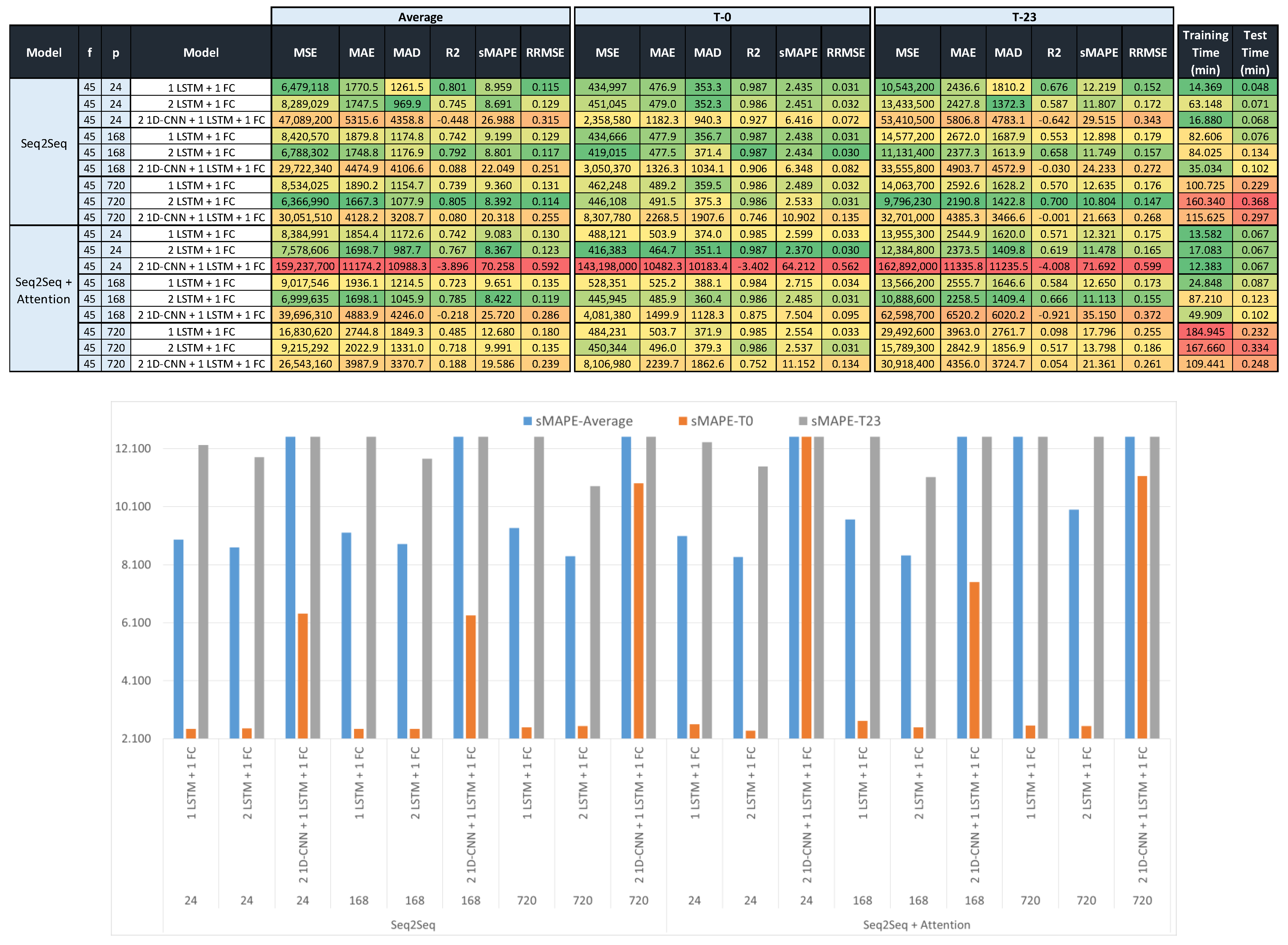
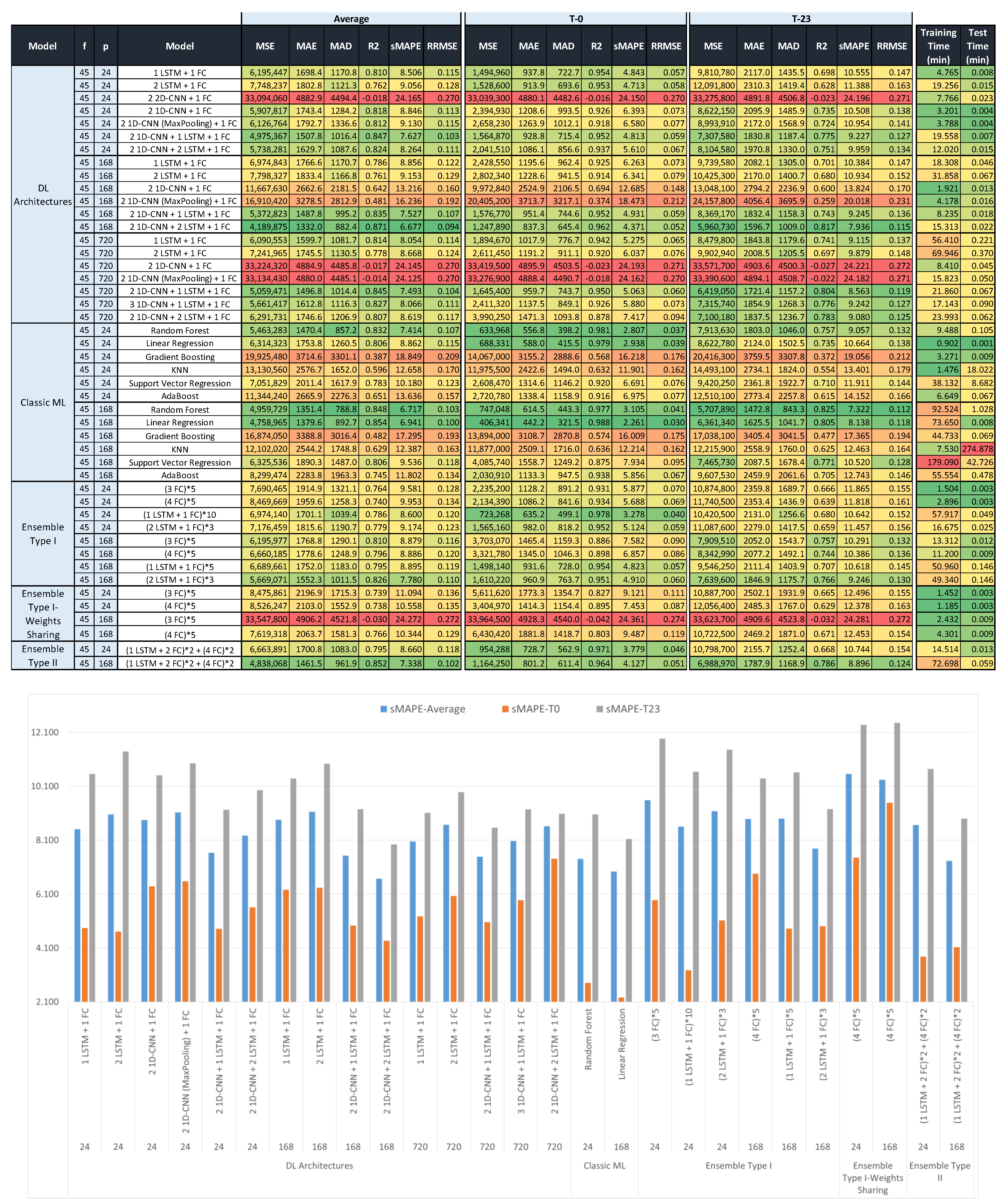
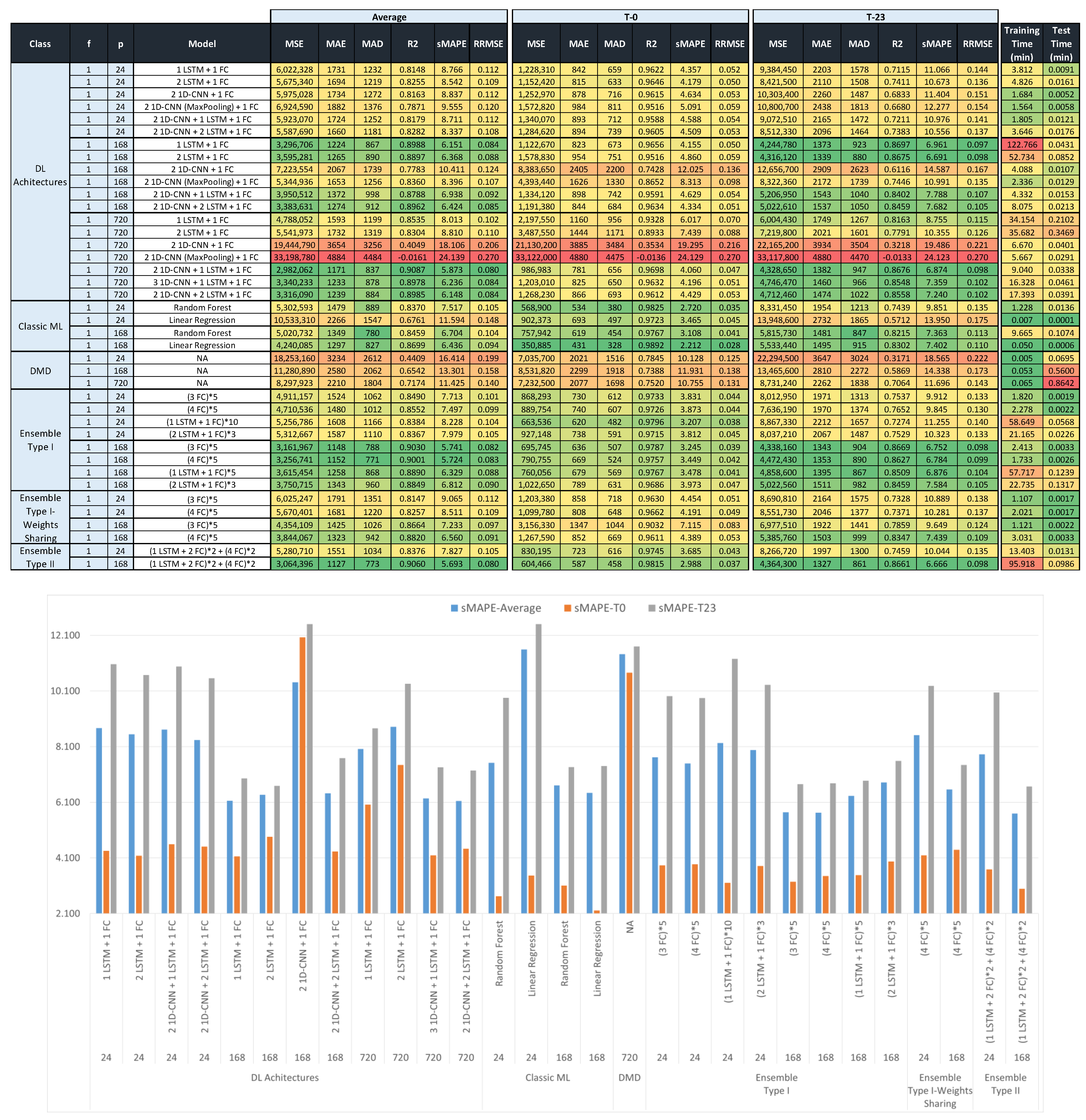
Figure 6, Figure 7 and Figure 8 show the forecast metrics for the different models (Section 3.2), and for different values of the parameters $f$, $p$, and $k$. They present the data in two sections, with the upper section presenting the raw data with a color-code format, and the lower section showing a subset of the data in a bar chart format. The bar charts below the tables present the sMAPE metrics (average, T-0 and T-23) for some of the best performing models in the corresponding table. These tables present the metrics using a color code to easily show where the best values are. Color coding uses a color palette where the greenest color is for the best result and the reddest is for the worst. Color coding was applied column-wise to compare results for the same metric. Figure 6 presents all the results for the Seq2seq and Seq2seq + attention models. Figure 7 and Figure 8 present the results for the rest of the models, Figure 7 for a $f$ value equal to 45, and Figure 8 for an $f$ value equal to 1. Metric values are provided for the forecasts of the first (T-0) and the last (T-23) time-slots, in addition to the average of forecasts for all (24) predicted time-slots. The last two columns provide the training and test times for all models.

Figure 6. (Upper section): forecast metrics for the average, first (T-0), and last (T-23) predicted time-slots using Seq2seq with and without an attention mechanism. The table is color-coded along columns with colors between red and green corresponding to the worst and best results, respectively. (Lower section): bar chart for sMAPE metrics for some of the best performing models from the upper table.

Figure 7. (Upper section): forecast metrics for the average, first (T-0), and last (T-23) predicted time-slots using DL, ML, and ensemble models for a fixed number of values per predictor ($f$ = 45). The table is color-coded along columns with colors between red and green corresponding to the worst and best results, respectively. (Lower section): bar chart for sMAPE metrics for some of the best performing models from the upper table.

Figure 8. (Upper section): forecast metrics for the average, first (T-0), and last (T-23) predicted time-slots using DL, ML, and ensemble models for a fixed number of values per predictor ($f$ = 1). The table is color-coded along columns with colors between red and green corresponding to the worst and best results, respectively. (Lower section): bar chart for sMAPE metrics for some of the best performing models from the upper table.

The best results for the Seq2seq models were achieved when using only recurring networks (one or two LSTM layers) while the inclusion of convolutional layers deteriorates the forecast. Seq2seq models (Figure 6 and Figure A1 (Appendix A) present some of the best results for very short-term forecasts and worst for average and long-term forecasts. These models have difficulty converging with $f$, equal to one with their best results with $f$equal to 45.

The results for DL, ML, and ensemble models, with an $f$ value equal to 45, are shown in Figure 7 and the Appendix A. For this value of parameter $f$, the best performing models were classic ML models. A combination of two CNN layers and two LSTM appeared to provide a performance similar to random forest and linear regression. The ensemble models did not give a good performance either.

The results for DL, ML, and ensemble models, with an $f$ value equal to 1, are shown in Figure 8 and the Appendix A. The results in this figure are very different from the results in Figure 7, despite being the same models with a different value for parameter $f$. In Figure 8, we obtain most of the best results obtained in this work. The best performing model types were DL and ensemble models for long-term forecasting and average results, while for short-term results, the classic ML and Seq2seq models were best. It is interesting how the combination of CNN and LSTM layers produced some of the best performance models, since this result is very different from what happens in Seq2seq architectures, for which these layer combinations provide very poor results.

A conclusion drawn from the results in Figure 6, Figure 7 and Figure 8 is the importance of the impact of the rolling window length and the number of features associated with the time-slots. Another is that the best specific sequence of layers for a deep learning architecture depends on the type of model, making it impossible to establish a priori a better architecture for all types of models.

In all the tables in Figure 6, Figure 7 and Figure 8, the description of the models includes the number and type of layers used: CNN, LSTM, and fully connected layers (FC), forming a sequence separated by the + sign. The ensemble models follow the gaNet architecture [11] which is formed by repeating blocks where the configuration of each repeating block is included in parentheses with an asterisk and a number to the right of the parentheses that indicates the number of repetitions of the block. Ensemble Type II models that are made up of different blocks with a possibly different architecture per block can also have different types of inputs per block; in those cases where there are different inputs per block, we have marked that in the tables by an NA in the $f$ column, reporting the type of input associated with each block by an additional letter within parentheses and immediately after the layer type (LSTM or 1D-CNN). Possible values for these additional letters are: an (L) for inputs formed exclusively by the load values, a (D) for inputs formed by the load plus the date/time features, and a (A) for inputs formed by the load plus the date/time and weather features.

Table 1 provides a summary table with a ranking of the three best models for the three most important metrics ($R^2$, RRMSE, and SMAPE) plus training and test times. Similar to Figure 6, Figure 7 and Figure 8, metric values are provided for the forecasts of the first (T-0) and the last (T-23) time-slots, in addition to the average of forecasts for all (24) predicted time-slots.

Table 1. Ranking of the three best models for the three most important metrics ($R^2$, SMAPE and RRMSE) plus training and test times. Values are provided for the forecasts of the first (T-0) and the last (T-23) time-slots, in addition to the average of forecasts for all (24) predicted time-slots.

	Metric	Rank	Class	f	p	k	Model	Metric Value
Average	$R^2$	1°	DL Achitectures	1	720	24	2 1D-CNN + 1 LSTM + 1 FC	0.9087
		2°	Ensemble Type II	1	168	24	(1 LSTM + 2 FC) * 2 + (4 FC) * 2	0.9060
		3°	Ensemble Type I	1	168	24	(3 FC) * 5	0.9030
	sMAPE	1°	Ensemble Type II	1	168	24	(1 LSTM + 2 FC) * 2 + (4 FC) * 2	5.6934
		2°	Ensemble Type I	1	168	24	(4 FC) * 5	5.7235
		3°	Ensemble Type I	1	168	24	(3 FC) * 5	5.7410
	RRMSE	1°	DL Achitectures	1	720	24	2 1D-CNN + 1 LSTM + 1 FC	0.0797
		2°	Ensemble Type II	1	168	24	(1 LSTM + 2 FC) * 2 + (4 FC)*2	0.0803
		3°	Ensemble Type I	1	168	24	(3 FC) * 5	0.0820
T-0	$R^2$	1°	Classic ML	1	168	24	Linear Regression	0.9892
		2°	Classic ML	45	168	24	Linear Regression	0.9875
		3°	Seq2Seq + Attention	45	24	24	2 LSTM + 1 FC	0.9872
	sMAPE	1°	Classic ML	1	168	24	Linear Regression	2.2120
		2°	Classic ML	45	168	24	Linear Regression	2.2608
		3°	Seq2Seq + Attention	45	24	24	2 LSTM + 1 FC	2.3705
	RRMSE	1°	Classic ML	1	168	24	Linear Regression	0.0278
		2°	Classic ML	45	168	24	Linear Regression	0.0299
		3°	Seq2Seq + Attention	45	24	24	2 LSTM + 1 FC	0.0303
T-23	R2	1°	DL Achitectures	1	168	24	1 LSTM + 1 FC	0.8697
		2°	DL Achitectures	1	720	24	2 1D-CNN + 1 LSTM + 1 FC	0.8676
		3°	DL Achitectures	1	168	24	2 LSTM + 1 FC	0.8675
	sMAPE	1°	Ensemble Type II	1	168	24	(1 LSTM + 2 FC) * 2 + (4 FC) * 2	6.6660
		2°	DL Achitectures	1	168	24	2 LSTM + 1 FC	6.6912
		3°	Ensemble Type I	1	168	24	(3 FC) * 5	6.7516
	RRMSE	1°	DL Achitectures	1	168	24	1 LSTM + 1 FC	0.0967
		2°	DL Achitectures	1	720	24	2 1D-CNN + 1 LSTM + 1 FC	0.0975
		3°	DL Achitectures	1	168	24	2 LSTM + 1 FC	0.0976
	Training Time (min)	1°	DMD	1	24	24	NA	0.0047
		2°	Classic ML	1	24	24	Linear Regression	0.0066
		3°	Classic ML	1	168	24	Linear Regression	0.0499
	Test Time (min)	1°	Classic ML	1	24	24	Linear Regression	0.0001
		2°	Classic ML	1	168	24	Linear Regression	0.0006
		3°	Ensemble Type I-B	1	24	24	(3 FC) * 5	0.0017

The main findings of the work, as conclusions from Table 1, are:

• The best value for parameter $p$ seems to be 168, i.e., having a rolling window length of 1 week, it appears that shorter and longer values do not generally provide the best results. The exceptions are Seq2seq models, which prefer a value of 24 (1 day), and some deep learning models that combine a CNN with an LSTM, for which 720 (1 month) is the preferred length.
• The best number of features associated with each time-slot seems to be one, i.e., to use the load value exclusively. The exception is again the Seq2seq models which prefer to have the date features additionally. The behavior of logistic regression is confusing in this regard because they obtain best results with both 1 and 45 features/time-slot.
• For near-term forecasts (prediction of the following value), the linear/simple models, as linear regression, provide the best results when using a large enough number of predictors ($p$ = 128) and a simple scalar predictor value ($f$ = 1), which is the electric load. In this scenario, another model providing the best results is the Seq2seq+attention model with a smaller number of predictors ($p$ = 24) and the full vector of predictor values ($f$ = 45).
• For longer-term forecasts, the deep learning models with one or two LSTM layers provide the best results. Another model with excellent performance is a model combining 1D-CNN layers and LSTM layers. The model with the best sMAPE metric is an ensemble Type II model with a small number of dense and LSTM blocks. In all these cases, the best results are obtained with a large number of predictors ($p$ = 168, 720) and a smaller number of values per predictor ($f$ = 1).
• Considering the average results for the 24 predicted values, the best results are obtained for: (1) ensemble Type II models with a small number of dense and LSTM blocks, (2) ensemble Type I models with a small number of dense blocks, and (3) combined 1D-CNN and LSTM layers with $p$ = 720. All these results are obtained with the smaller number of values per predictor ($f$ = 1).
• Interestingly, multiple output models can produce better results for distant forecasts than single output models (classic ML models) even when the latter models have a specific regressor to predict each output. This is a demonstration of the great correlation between the outputs that a single model can learn, while $k$ independent regressors lose this valuable information.

In Figure A1 (Appendix A), a complete table is provided, integrating the results from Figure 6, Figure 7 and Figure 8 into a single one. The Table in the Appendix A contains additional results that are not shown in Figure 6, Figure 7 and Figure 8, with the intention to simplify them by not showing the worst performing models.

Another interesting result is that including additional features (date/time, weather) should provide an improvement in the results due to the strong correlation between weather and electricity consumption. Nevertheless, this influence turned out to be less significant than anticipated, with most models performing better simply by using the past load values. An explanation could be obtained from the results presented in previous works showing that the influence of weather data is more noticeable as the forecast period increases [36,37], and their influence is small for a forecast horizon of a few hours [37].

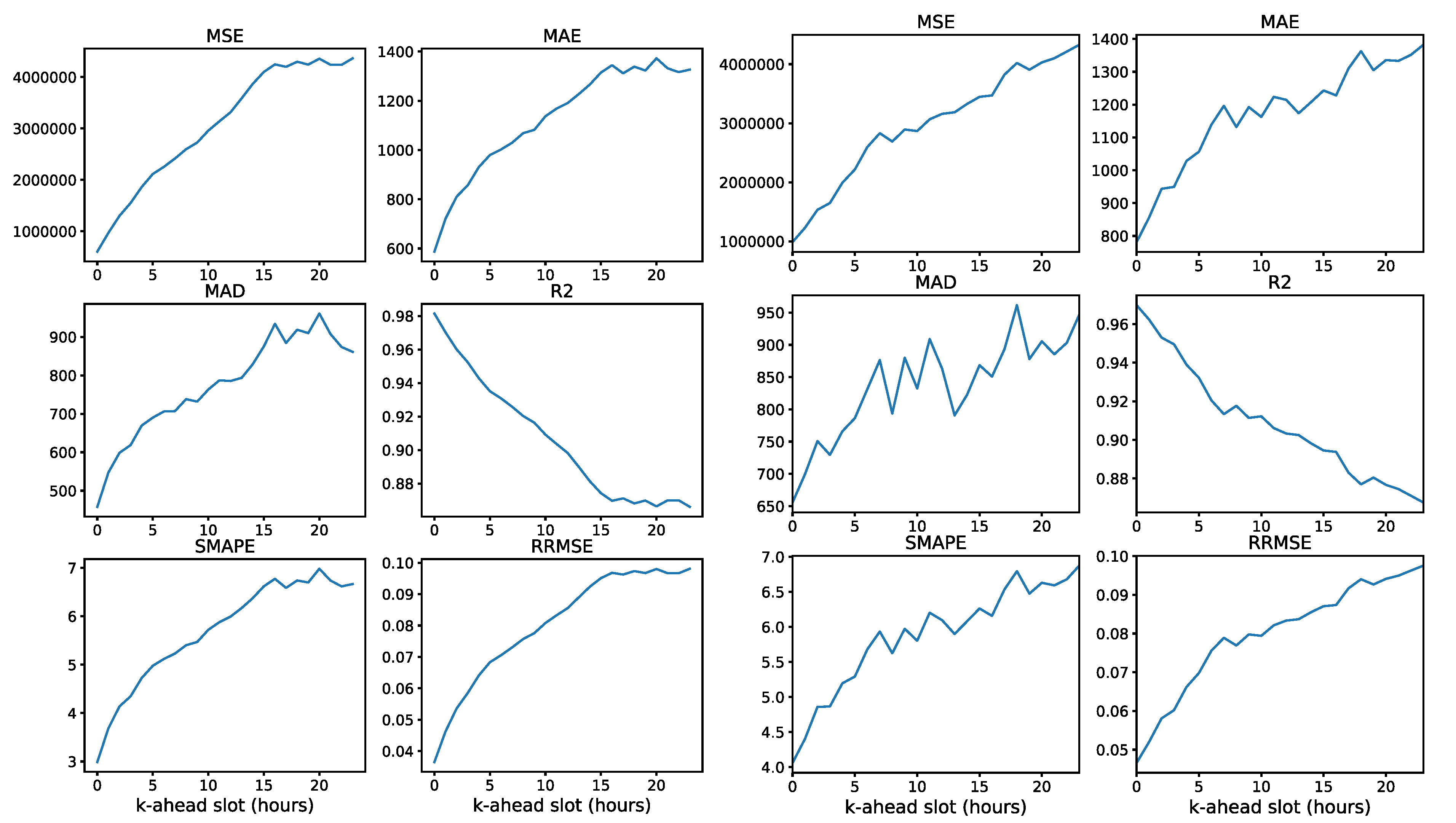
It is interesting to analyze the evolution of the forecast metrics for the different time-ahead time-slots. This evolution depends mainly on the forecasting model, and it can range from a monotonous decreasing line to a decreasing exponential, and it can have intermediate plateaus where the performance is almost constant regardless of the prediction time distance. In all cases, the performance metrics experience a decline when the forecast is for a longer time interval, as intuitively expected. Figure 9 presents the evolution of the forecast metrics for different k-ahead forecasts for two of the best models for average forecasting (Table 1) and Figure 10 for another two of the best models for near-term forecasting (Table 1).

Figure 9. Forecast metrics for successive predicted time-slots for models: ensemble Type II ((1 LSTM + 2 FC) * 2 + (4 FC) * 2) ($f$ = 1, $p$ = 168, $k$ = 24) (left) and DL architecture (2 1D-CNN + 1 LSTM + 1 FC) ($f$ = 1, $p$ = 720, $k$ = 24) (right).

Figure 10. Forecast metrics for successive predicted time-slots for models: classic ML, (linear regression) ($f$ = 1, $p$ = 168, $k$ = 24) (left) and Seq2seq + attention (2 LSTM + 1 FC) ($f$ = 45, $p$ = 24, $k$ = 24) (right).

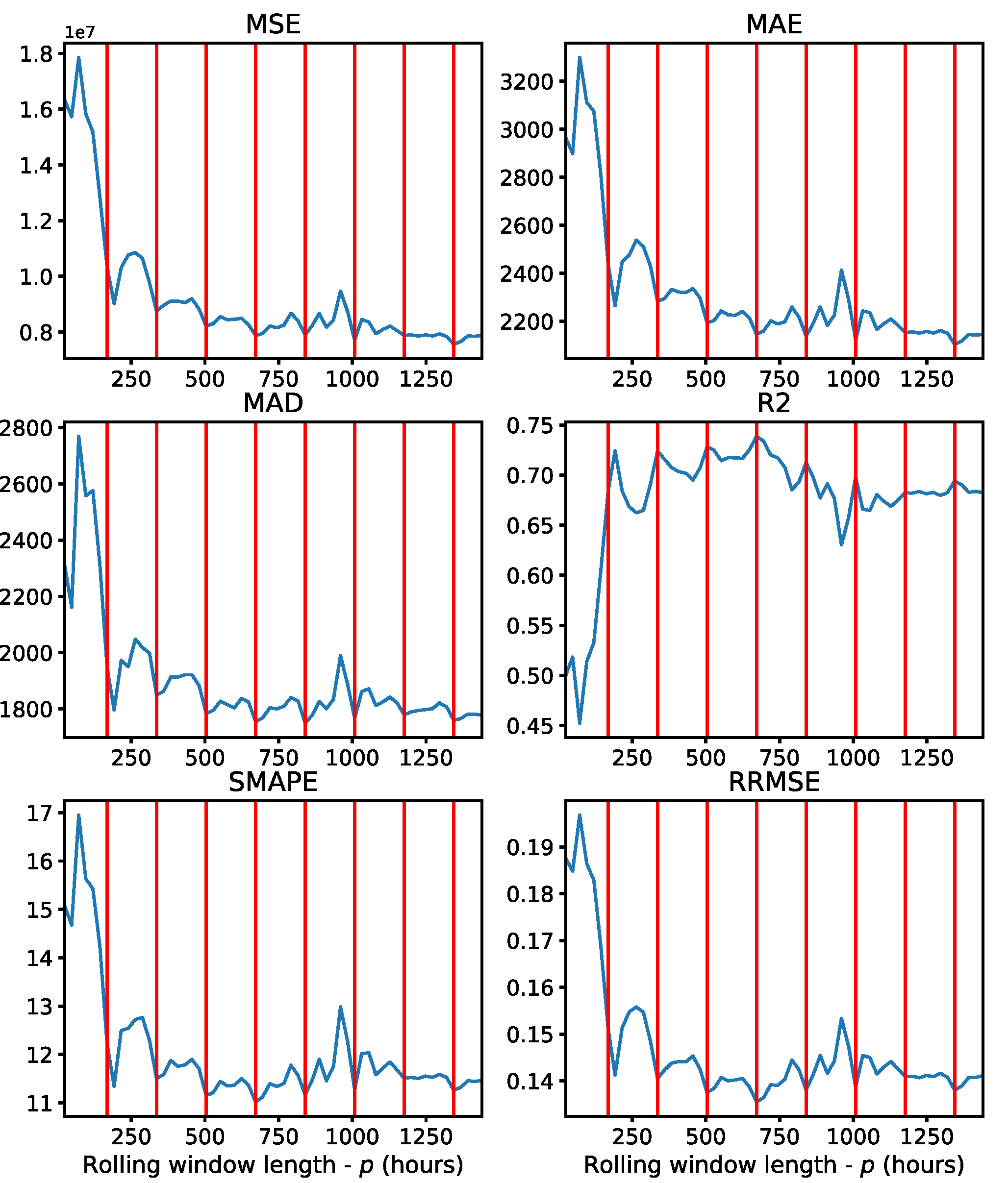
It is interesting to analyze the impact of the rolling window length (parameter $p$) on the forecast performance metrics. Figure 11 presents the impact on the performance metrics with a rolling window length between 24 (1 day) and 1440 h (60 days). In Figure 11, a vertical red line marks an interval of one week (168 h). A performance improvement is obtained by increasing the value of $p$ up to a value of 168 (1 week of rolling window length); from this point, the improvement is much smaller, and even decreases with a $p$ value greater than 720 (4 weeks). This behavior explains why the best results were obtained with a $p$ value between 168 and 720. The Seq2seq models are an exception in this case due to their difficulties in handling large input vectors.

Figure 11. Influence of the rolling window length ($p$) on different forecast metrics (MSE, MAE, MAD, $R^2$, SMAPE and RRMSE), obtained with the DMD model. The range of values for $p$ is between 24 (1 day) and 1440 h (60 days).

It may also be of interest to investigate the evolution of the loss function during training. Figure 12 provides this evolution for one of the deep learning architectures ((1 LSTM + 1 FC) ($f$ = 1, $p$ = 168, $k$ = 24)), using the mean squared error (MSE) loss. In general, we observed that after 20–30 epochs, most of the models converged smoothly, with the Seq2seq and ensemble models experiencing the most difficulties in their convergence.

Figure 12. Training (blue line) and validation (green line) MSE loss evolution for successive epochs while training (model: DL architecture (1 LSTM + 1 FC) ($f$ = 1, $p$ = 168, $k$ = 24)).

To provide a visual indication of the quality of the 24 h forecast, Figure 13 shows a comparison between real (ground-truth) load signals and their forecasts as we increase the forecast time horizon. The different diagrams are 24 h time windows taken at random points in the test set. The forecast follows the real signal almost perfectly to a point where it begins to drift. The drift point is different for different samples, with some signals perfectly followed almost all the time and others beginning to separate in the initial forecasts. In all cases, the forecast signal is a smoothed version of the real one.

Figure 13. Comparison between real 24 h load signals (blue lines) and their forecasts (orange lines) for data in the test set (model: ensemble Type II ([1 LSTM + 2 FC] * 2 + (4 FC) * 2) ($f$ = 1, $p$ = 168, $k$ = 24)).

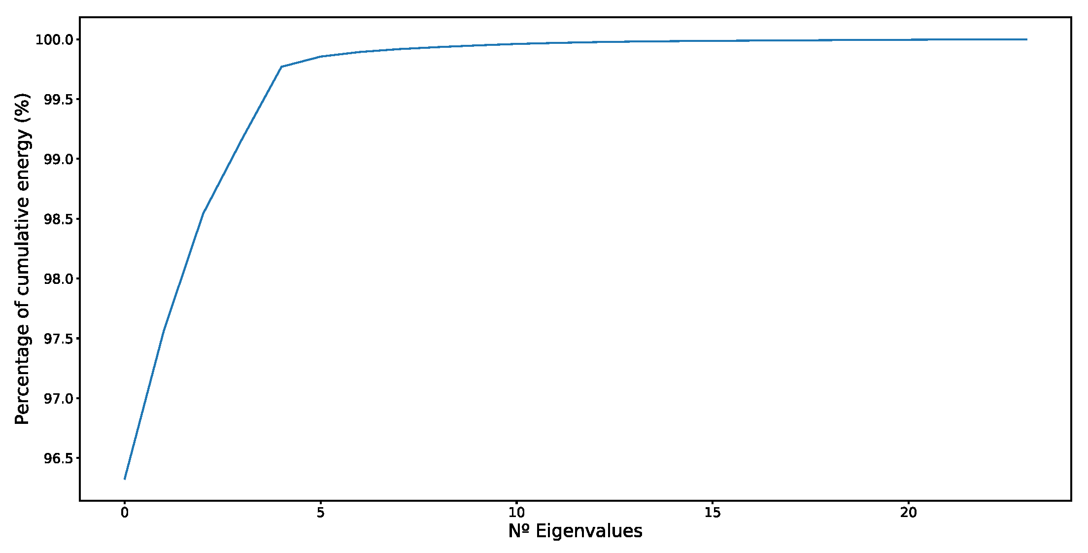
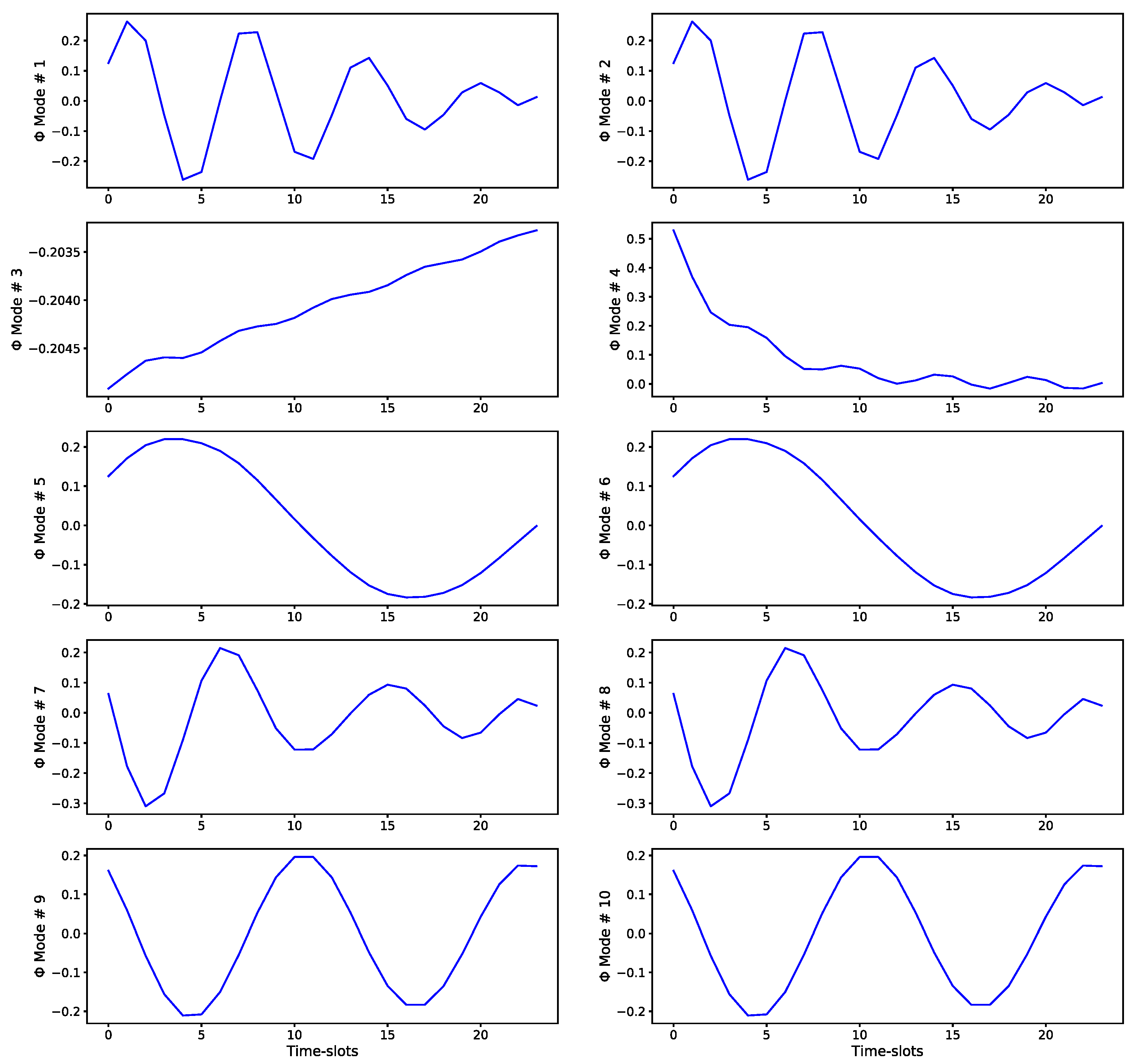
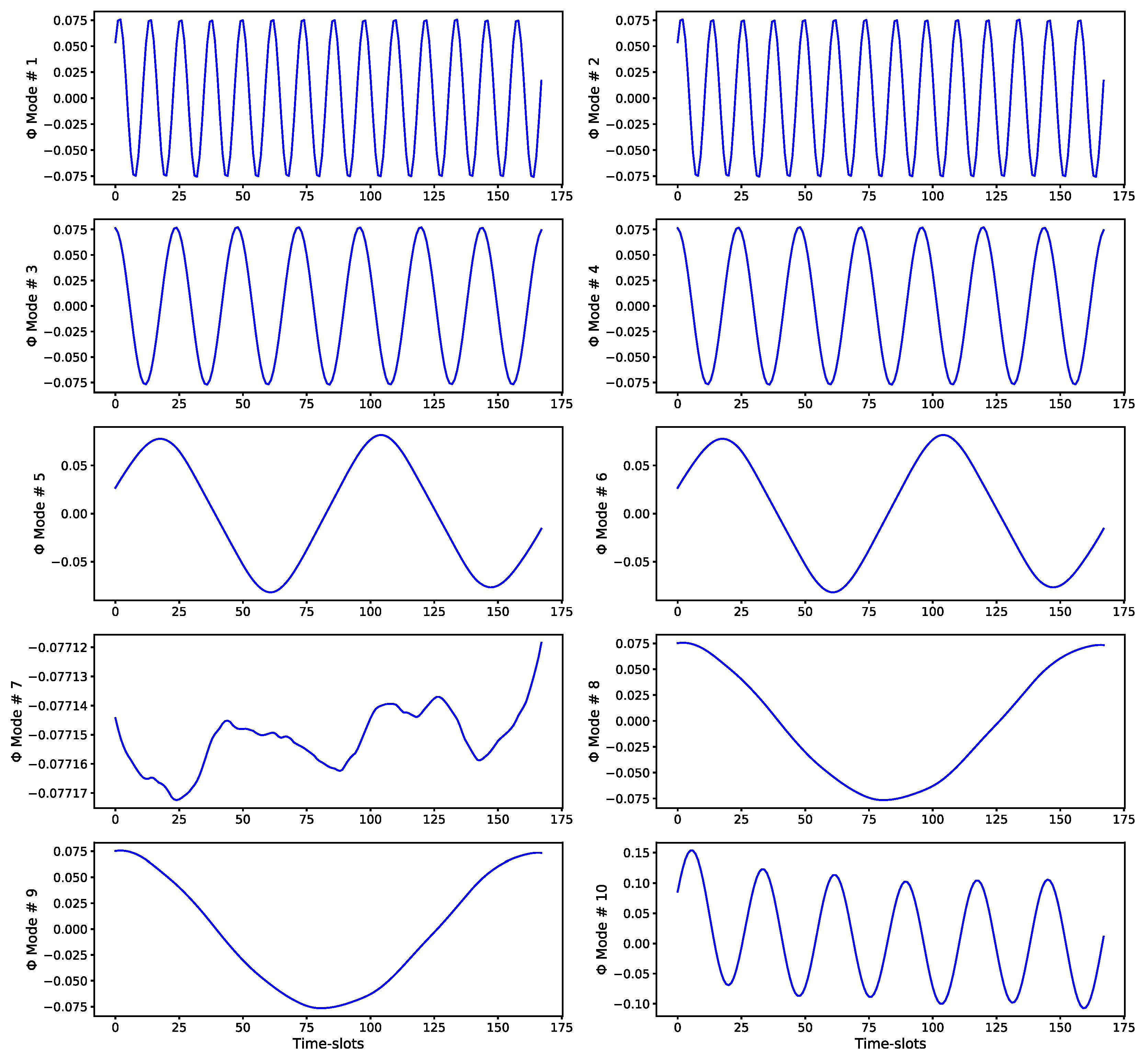
Figure 14, Figure 15, Figure 16 and Figure 17 present the ability of the DMD algorithm to identify the structure of the time-series (load values). Figure 14 shows the evolution of the signal energy (sum of squares of principal eigenvalues) in relation to the total signal energy (sum squares of all eigenvalues). We observe that to achieve a 99% total signal energy, generally a few eigenvalues are sufficient. In particular, for our dataset, 10 eigenvalues (modes) are sufficient to capture the 99% of total signal energy for a rolling window of 24 and 168 h, and 16 eigenvalues for a rolling window of 720 h.

Figure 14. Graph showing the total energy of the signal captured by the linear DMD approximation versus the number of eigenvectors (modes) used to implement the transformation. This graph was obtained with a rolling window of 24 h, and is very similar to the graph for a rolling window of 168 h.

Figure 15. Principal eigenvectors ($\mathsf{\Phi }$) of the DMD algorithm (best linear mapping) for the temporal evolution of the load values. The eigenvectors are in order of importance (according to their corresponding eigenvalues) and represent the main modes of temporal evolution of the time-series. They clearly show the strong intra-day periodicity of the load values. The values shown correspond to a rolling window of 24 h (1 day).

Figure 16. Principal eigenvectors ($\mathsf{\Phi }$) of the DMD algorithm (best linear mapping) for the temporal evolution of the load values. The eigenvectors are in order of importance (according to their corresponding eigenvalues) and represent the main modes of temporal evolution of the time-series. They clearly show the strong daily periodicity of the load values. The values shown correspond to a rolling window of 168 h (1 week).

Figure 17. Principal eigenvectors ($\mathsf{\Phi }$) of the DMD algorithm (best linear mapping) for the temporal evolution of the load values. The eigenvectors are in order of importance (according to their corresponding eigenvalues) and represent the main modes of temporal evolution of the time-series. They clearly show the strong daily/weekly periodicity of the load values. The values shown correspond to a rolling window of 720 h (1 month). In this case, 16 eigenvectors were needed to capture 99% of the total signal energy.

Figure 15, Figure 16 and Figure 17 show the principal eigenvectors ($\mathsf{\Phi }$) of the DMD algorithm for the temporal evolution of the load values and for different rolling window lengths (24, 168, and 720 h). The eigenvectors are in order of importance (according to their corresponding eigenvalues) and represent the main modes of temporal evolution of the time-series. They show the strong periodicity of the load values at different levels of granularity: intra-day, daily, and weekly.

We implemented all the neural network models (deep learning, Seq2seq, attention, and gaNet) in python using Tensorflow/Keras [59]. For all other models, we used the scikit-learn python package [60].

5. Conclusions

This work provides a comprehensive analysis of a significant number of novel forecasting models from different fields and areas of research, exploring reduced-order dynamical systems techniques (DMD), classic ML models (linear regression, random forest, gradient boosting, k-nearest neighbors, support vector regression, and AdaBoost), DL models (convolutional and recurrent architectures and their combination), DL sequence to sequence models (Seq2seq with and without attention), and specific DL ensemble models (gaNet). All techniques were applied to a unique dataset obtained from real data from a Spanish utility, which implies having a homogeneous set of results that allows a systematic comparison between models.

Some of the models analyzed have been widely applied to STLF (e.g., classical machine learning models), while others have rarely been applied (e.g., sequence to sequence, attention, DMD), and some of them have been applied for the first time to STLF, as far as we know (e.g., deep learning ensemble models specifically suitable for time-series forecasting, and specific configurations combining convolutional and recurring layers).

The main conclusions obtained from this work are the following: (a) A rolling window of 1 week appears to be the best value for most models, and longer and shorter values do not, on average, provide better results. (b) Another interesting result is that including additional features (date/time, weather) could provide an improvement in the results in some scenarios, but not in general, the models that obtain better results simply using the past values of load being more numerous. (c) For very-short term forecasts, it is important to note that simple linear models and Seq2seq architectures provide better results than more complex models. (d) For longer-term forecasts, deep learning models consisting of convolutional layers followed by recurrent layers provide the best results, better than pure convolutional or recurrent networks and similar, in forecasting performance in DL ensemble models (gaNet). (e) When the focus is to have good average forecasts, considering both very short-term and medium-term forecasts, the best models are DL ensemble models (gaNet), followed by CNN/RNN network combinations.

This work also validates the importance of deep ensemble models and how they provide better performance results for predictions with increasing degrees of uncertainty. It corroborates other studies that try to understand the foundations of this behavior, considering different points of view. This work presents a specific deep ensemble model that originated by combining ideas from gradient boosting and residual networks [11] and demonstrates the results from other ensemble architectures [27,61] where emphasis is placed on the random initialization of the different ensemble entities.

As already mentioned, the electrical sector is a critical infrastructure and therefore one of the main industries exposed to security and fraud attacks, i.e., DDoS (distributed denial of service) cybersecurity threats. It could also be vulnerable to so-called ransomware cybersecurity attacks, where the attacker hijacks (typically through encryption) customer data that can only be recovered after payment to the attacker. One specific threat scenario is related to charging and billing. In smart grids, the central billing system receives customer consumptions from so-called smart meters through communication technologies. It also receives aggregated consumptions from intermediate elements of the grid (substations at district level, city distribution level). A cybersecurity attack could target both the billing system and the individual smart meters, preventing the electrical utility from knowing how much electricity has been consumed by the customers. An electrical company would lose a significant amount of money if it was not able to bill its customers, and the attacker could ask for an important ransom. However, thanks to machine learning, the electrical company could estimate the consumption made based on historical data, and therefore, minimize the incentive of the attacker to ask for a ransom, and if the attack is executed in any case, make a provisional billing based on an accurate estimation. With the current dataset, estimations are made at the small city level, because consumption data from individual smart meters are much more restrictive from a General Data Protection Regulation (European Union) data privacy perspective. As a future line of study, research could be extended with anonymized personal identifiable information.

Considering the experience gained with deep learning models applied to time-series forecasting from the perspective of a multivariate multi-output regression problem, we plan to extend the experiments with novel deep learning sequential models, such as transformers [62]. Another future work will be to build controlled perturbation-based experiments to demonstrate the capabilities of STLF as a security/threat indicator.

References

1. Nguyen, H.; Hansen, C.K. Short-term electricity load forecasting with Time Series Analysis. In Proceedings of the 2017 IEEE International Conference on Prognostics and Health Management (ICPHM), Dallas, TX, USA, 19–21 June 2017; pp. 214–221. [Google Scholar]
2. Hernández, L.; Baladron, C.; Aguiar, J.M.; Carro, B.; Sanchez-Esguevillas, A.J.; Lloret, J.; Massana, J. A Survey on Electric Power Demand Forecasting: Future Trends in Smart Grids, Microgrids and Smart Buildings. IEEE Commun. Surv. Tutor. 2014, 16, 1460–1495. [Google Scholar] [CrossRef]
3. Schmid, P.J. Dynamic mode decomposition of numerical and experimental data. J. Fluid Mech. 2010, 656, 5–28. [Google Scholar] [CrossRef]
4. Tirunagari, S.; Kouchaki, S.; Poh, N.; Bober, M.; Windridge, D.; Dynamic, D.W. Dynamic Mode Decomposition for Univariate Time Series: Analysing Trends and Forecasting. 2017. Available online: https://hal.archives-ouvertes.fr/hal-01463744 (accessed on 18 June 2021).
5. Mohan, N.; Soman, K.P.; Sachin Kumar, S. A data-driven strategy for short-term electric load forecasting using dynamic mode decomposition model. Appl. Energy 2018, 232, 229–244. [Google Scholar] [CrossRef]
6. Lopez-Martin, M.; Carro, B.; Sanchez-Esguevillas, A.; Lloret, J. Network Traffic Classifier with Convolutional and Recurrent Neural Networks for Internet of Things. IEEE Access 2017, 5. [Google Scholar] [CrossRef]
7. Lopez-Martin, M.; Carro, B.; Lloret, J.; Egea, S.; Sanchez-Esguevillas, A. Deep Learning Model for Multimedia Quality of Experience Prediction Based on Network Flow Packets. IEEE Commun. Mag. 2018, 56. [Google Scholar] [CrossRef]
8. Sutskever, I.; Vinyals, O.; Le, Q.V. Sequence to Sequence Learning with Neural Networks. arXiv 2014, arXiv:1409.3215. [Google Scholar]
9. Bahdanau, D.; Cho, K.; Bengio, Y. Neural Machine Translation by Jointly Learning to Align and Translate. arXiv 2014, arXiv:1409.0473. [Google Scholar]
10. Luong, M.-T.; Pham, H.; Manning, C.D. Effective Approaches to Attention-based Neural Machine Translation. arXiv 2015, arXiv:1508.04025. [Google Scholar]
11. Lopez-Martin, M.; Carro, B.; Sanchez-Esguevillas, A. Neural network architecture based on gradient boosting for IoT traffic prediction. Future Gener. Comput. Syst. 2019, 100, 656–673. [Google Scholar] [CrossRef]
12. Bontempi, G.; Ben Taieb, S.; Le Borgne, Y.-A. Machine Learning Strategies for Time Series Forecasting BT-Business Intelligence: Second European Summer School, eBISS 2012, Brussels, Belgium, 15–21 July 2012. In Tutorial Lectures; Aufaure, M.-A., Zimányi, E., Eds.; Springer: Berlin/Heidelberg, Germany, 2013; pp. 62–77. ISBN 978-3-642-36318-4. [Google Scholar]
13. Bourdeau, M.; Zhai, X.Q.; Nefzaoui, E.; Guo, X.; Chatellier, P. Modeling and forecasting building energy consumption: A review of data-driven techniques. Sustain. Cities Soc. 2019, 48, 101533. [Google Scholar] [CrossRef]
14. Makridakis, S.; Spiliotis, E.; Assimakopoulos, V. Statistical and Machine Learning forecasting methods: Concerns and ways forward. PLoS ONE 2018, 13, e0194889. [Google Scholar] [CrossRef]
15. Martin, M.L.; Sanchez-Esguevillas, A.; Carro, B.C. Review of Methods to Predict Connectivity of IoT Wireless Devices. In Ad Hoc and Sensor Wireless Networks; Old City Publishing, Inc.: Philadelphia, PA, USA, 2017; Volume 38, pp. 125–141. [Google Scholar]
16. Hernández, L.; Baladrón, C.; Aguiar, J.M.; Carro, B.; Sánchez-Esguevillas, A.; Lloret, J. Artificial neural networks for short-term load forecasting in microgrids environment. Energy 2014, 75, 252–264. [Google Scholar] [CrossRef]
17. Hernández, L.; Baladrón, C.; Aguiar, J.; Calavia, L.; Carro, B.; Sánchez-Esguevillas, A.; Pérez, F.; Fernández, Á.; Lloret, J. Artificial Neural Network for Short-Term Load Forecasting in Distribution Systems. Energies 2014, 7, 1576–1598. [Google Scholar] [CrossRef]
18. Hernández, L.; Baladrón, C.; Aguiar, J.; Calavia, L.; Carro, B.; Sánchez-Esguevillas, A.; Sanjuán, J.; González, Á.; Lloret, J. Improved Short-Term Load Forecasting Based on Two-Stage Predictions with Artificial Neural Networks in a Microgrid Environment. Energies 2013, 6, 4489–4507. [Google Scholar] [CrossRef]
19. Hernández, L.; Baladrón, C.; Aguiar, J.; Calavia, L.; Carro, B.; Sánchez-Esguevillas, A.; García, P.; Lloret, J. Experimental Analysis of the Input Variables’ Relevance to Forecast Next Day’s Aggregated Electric Demand Using Neural Networks. Energies 2013, 6, 2927–2948. [Google Scholar] [CrossRef]
20. Hernández, L.; Baladrón, C.; Aguiar, J.; Carro, B.; Sanchez-Esguevillas, A.; Lloret, J. Short-Term Load Forecasting for Microgrids Based on Artificial Neural Networks. Energies 2013, 6, 1385–1408. [Google Scholar] [CrossRef]
21. Hernández, L.; Baladron, C.; Aguiar, J.M.; Carro, B.; Sanchez-Esguevillas, A.; Lloret, J.; Chinarro, D.; Gomez-Sanz, J.J.; Cook, D. A multi-agent system architecture for smart grid management and forecasting of energy demand in virtual power plants. IEEE Commun. Mag. 2013, 51, 106–113. [Google Scholar] [CrossRef]
22. Hernández, L.; Baladrón, C.; Aguiar, J.; Carro, B.; Sánchez-Esguevillas, A. Classification and Clustering of Electricity Demand Patterns in Industrial Parks. Energies 2012, 5, 5215–5228. [Google Scholar] [CrossRef]
23. Hernández, L.; Baladrón, C.; Aguiar, J.M.; Calavia, L.; Carro, B.; Sánchez-Esguevillas, A.; Cook, D.J.; Chinarro, D.; Gómez, J. A Study of the Relationship between Weather Variables and Electric Power Demand inside a Smart Grid/Smart World Framework. Sensors 2012, 12, 11571–11591. [Google Scholar] [CrossRef]
24. Lopez-Martin, M.; Carro, B.; Sanchez-Esguevillas, A. IoT type-of-traffic forecasting method based on gradient boosting neural networks. Future Gener. Comput. Syst. 2020, 105, 331–345. [Google Scholar] [CrossRef]
25. Wolpert, D.H. Stacked generalization. Neural Netw. 1992, 5, 241–259. [Google Scholar] [CrossRef]
26. He, K.; Zhang, X.; Ren, S.; Sun, J. Deep Residual Learning for Image Recognition. In Proceedings of the 2016 IEEE Conference on Computer Vision and Pattern Recognition (CVPR), Las Vegas, NV, USA, 27–30 June 2016; pp. 770–778. [Google Scholar]
27. Frankle, J.; Carbin, M. The Lottery Ticket Hypothesis: Finding Sparse, Trainable Neural Networks. arXiv 2018, arXiv:1803.03635. [Google Scholar]
28. Jain, S.; Liu, G.; Mueller, J.; Gifford, D. Maximizing Overall Diversity for Improved Uncertainty Estimates in Deep Ensembles. arXiv 2019, arXiv:1906.07380. [Google Scholar] [CrossRef]
29. Wang, W.; Lu, Z. Cyber security in the Smart Grid: Survey and challenges. Comput. Netw. 2013, 57, 1344–1371. [Google Scholar] [CrossRef]
30. Cui, L.; Qu, Y.; Gao, L.; Xie, G.; Yu, S. Detecting false data attacks using machine learning techniques in smart grid: A survey. J. Netw. Comput. Appl. 2020, 170, 102808. [Google Scholar] [CrossRef]
31. Zhang, L.; Wen, J.; Li, Y.; Chen, J.; Ye, Y.; Fu, Y.; Livingood, W. A review of machine learning in building load prediction. Appl. Energy 2021, 285, 116452. [Google Scholar] [CrossRef]
32. Zhao, Y.; Zhang, C.; Zhang, Y.; Wang, Z.; Li, J. A review of data mining technologies in building energy systems: Load prediction, pattern identification, fault detection and diagnosis. Energy Built Environ. 2020, 1, 149–164. [Google Scholar] [CrossRef]
33. Vivas, E.; Allende-Cid, H.; Salas, R. A Systematic Review of Statistical and Machine Learning Methods for Electrical Power Forecasting with Reported MAPE Score. Entropy 2020, 22, 1412. [Google Scholar] [CrossRef] [PubMed]
34. Aguilar Madrid, E.; Antonio, N. Short-Term Electricity Load Forecasting with Machine Learning. Information 2012, 12, 50. [Google Scholar] [CrossRef]
35. Nti, I.K.; Teimeh, M.; Nyarko-Boateng, O.; Adekoya, A.F. Electricity load forecasting: A systematic review. J. Electr. Syst. Inf. Technol. 2020, 7, 1–19. [Google Scholar] [CrossRef]
36. Taylor, J.W. An evaluation of methods for very short-term load forecasting using minute-by-minute British data. Int. J. Forecast. 2008, 24, 645–658. [Google Scholar] [CrossRef]
37. Dumas, J.; Cornélusse, B. Classification of load forecasting studies by forecasting problem to select load forecasting techniques and methodologies. arXiv 2018, arXiv:1901.05052. [Google Scholar]
38. Hong, T.; Fan, S. Probabilistic electric load forecasting: A tutorial review. Int. J. Forecast. 2016, 32, 914–938. [Google Scholar] [CrossRef]
39. Hammad, M.A.; Jereb, B.; Rosi, B.; Dragan, D. Methods and Models for Electric Load Forecasting: A Comprehensive Review. Logist. Sustain. Transp. 2020, 11, 51–76. [Google Scholar] [CrossRef]
40. Kong, X.; Li, C.; Wang, C.; Zhang, Y.; Zhang, J. Short-term electrical load forecasting based on error correction using dynamic mode decomposition. Appl. Energy 2020, 261, 114368. [Google Scholar] [CrossRef]
41. Fan, C.; Ding, C.; Zheng, J.; Xiao, L.; Ai, Z. Empirical Mode Decomposition based Multi-objective Deep Belief Network for short-term power load forecasting. Neurocomputing 2020, 388, 110–123. [Google Scholar] [CrossRef]
42. Pinto, T.; Praça, I.; Vale, Z.; Silva, J. Ensemble learning for electricity consumption forecasting in office buildings. Neurocomputing 2020, 423, 747–755. [Google Scholar] [CrossRef]
43. Oprea, S.; Bâra, A. Machine Learning Algorithms for Short-Term Load Forecast in Residential Buildings Using Smart Meters, Sensors and Big Data Solutions. IEEE Access 2019, 7, 177874–177889. [Google Scholar] [CrossRef]
44. Jacob, M.; Neves, C.; Vukadinović Greetham, D. (Eds.) Short Term Load Forecasting BT-Forecasting and Assessing Risk Ndividual Electricity Peaks; Springer International Publishing: Cham, Switzerland, 2020; pp. 15–37. ISBN 978-3-030-28669-9. [Google Scholar]
45. Candelieri, A. Clustering and Support Vector Regression for Water Demand Forecasting and Anomaly Detection. Water 2017, 9, 224. [Google Scholar] [CrossRef]
46. Fan, S.; Hyndman, R.J. Short-Term Load Forecasting Based on a Semi-Parametric Additive Model. IEEE Trans. Power Syst. 2012, 27, 134–141. [Google Scholar] [CrossRef]
47. Gasparin, A.; Lukovic, S.; Alippi, C. Deep Learning for Time Series Forecasting: The Electric Load Case. arXiv 2019, arXiv:1907.09207. [Google Scholar]
48. Gong, G.; An, X.; Mahato, N.K.; Sun, S.; Chen, S.; Wen, Y. Research on Short-Term Load Prediction Based on Seq2seq Model. Energies 2019, 12, 3199. [Google Scholar] [CrossRef]
49. Du, S.; Li, T.; Yang, Y.; Horng, S.-J. Multivariate time series forecasting via attention-based encoder–decoder framework. Neurocomputing 2020, 388, 269–279. [Google Scholar] [CrossRef]
50. Huang, Y.; Wang, N.; Gao, W.; Guo, X.; Huang, C.; Hao, T.; Zhan, J. LoadCNN: A Low Training Cost Deep Learning Model for Day-Ahead Individual Residential Load Forecasting. arXiv 2019, arXiv:1908.00298. [Google Scholar]
51. Khotanzad, A.; Afkhami-Rohani, R.; Maratukulam, D. ANNSTLF-Artificial Neural Network Short-Term Load Forecaster- generation three. IEEE Trans. Power Syst. 1998, 13, 1413–1422. [Google Scholar] [CrossRef]
52. Farsi, B.; Amayri, M.; Bouguila, N.; Eicker, U. On Short-Term Load Forecasting Using Machine Learning Techniques and a Novel Parallel Deep LSTM-CNN Approach. IEEE Access 2021, 9, 31191–31212. [Google Scholar] [CrossRef]
53. Atef, S.; Eltawil, A.B. Assessment of stacked unidirectional and bidirectional long short-term memory networks for electricity load forecasting. Electr. Power Syst. Res. 2020, 187, 106489. [Google Scholar] [CrossRef]
54. Mann, J.; Kutz, J.N. Dynamic Mode Decomposition for Financial Trading Strategies. arXiv 2015, arXiv:1508.04487. [Google Scholar] [CrossRef]
55. Dylewsky, D.; Barajas-Solano, D.; Ma, T.; Tartakovsky, A.M.; Kutz, J.N. Dynamic mode decomposition for forecasting and analysis of power grid load data. arXiv 2020, arXiv:2010.04248. [Google Scholar]
56. He, X.; Zhao, K.; Chu, X. AutoML: A survey of the state-of-the-art. Knowl. Based Syst. 2021, 212, 106622. [Google Scholar] [CrossRef]
57. Zöller, M.-A.; Huber, M.F. Benchmark and Survey of Automated Machine Learning Frameworks. J. Artif. Int. Res. 2021, 70, 409–472. [Google Scholar] [CrossRef]
58. Hutter, F.; Kotthoff, L.; Vanschoren, J. (Eds.) Automated Machine Learning: Methods, Systems and Challenges; The Springer Series on Challenges in Machine Learning; Springer International Publishing: Cham, Switzerland, 2019; ISBN 978-3-030-05317-8. [Google Scholar]
59. Abadi, M.; Agarwal, A.; Barham, P.; Brevdo, E.; Chen, Z.; Citro, C.; Corrado, G.S.; Davis, A.; Dean, J.; Devin, M.; et al. TensorFlow: Large-Scale Machine Learning on Heterogeneous Distributed Systems. arXiv 2016, arXiv:1603.04467. [Google Scholar]
60. Pedregosa, F.; Michel, V.; Grisel, O.; Blondel, M.; Prettenhofer, P.; Weiss, R.; Vanderplas, J.; Cournapeau, D.; Pedregosa, F.; Varoquaux, G.; et al. Scikit-learn: Machine Learning in Python. J. Mach. Learn. Res. 2011, 12, 2825–2830. [Google Scholar]
61. Fort, S.; Hu, H.; Lakshminarayanan, B. Deep Ensembles: A Loss Landscape Perspective. arXiv 2019, arXiv:1912.02757. [Google Scholar]
62. Vaswani, A.; Brain, G.; Shazeer, N.; Parmar, N.; Uszkoreit, J.; Jones, L.; Gomez, A.N.; Kaiser, Ł.; Polosukhin, I. Attention Is All You Need. arXiv 2017, arXiv:1706.03762. [Google Scholar]
Publisher’s Note: MDPI stays neutral with regard to jurisdictional claims in published maps and institutional affiliations.
Article Metrics
Citations
Article Access Statistics
Multiple requests from the same IP address are counted as one view.