Review

Conventional and Deep Learning Methods for Skull Stripping in Brain MRI

1
Department of Mechatronics Engineering, Air University, Sector E-9, Islamabad 44000, Pakistan
2
School of Electrical Engineering, Hanyang University, Ansan 15588, Korea
*
Author to whom correspondence should be addressed.
Both authors contributed equally to this work.
Appl. Sci. 2020, 10(5), 1773; https://doi.org/10.3390/app10051773
Submission received: 14 January 2020 / Revised: 21 February 2020 / Accepted: 28 February 2020 / Published: 4 March 2020
(This article belongs to the Special Issue Computer-aided Biomedical Imaging 2020: Advances and Prospects)

Abstract

:

Featured Application

Skull stripping is the most prevalent brain image analysis method. This method can be applied to areas such as brain tissue segmentation and volumetric measurement, longitudinal analysis, multiple sclerosis analysis, cortical and sub-cortical analysis, assessing schizophrenia, and for the planning of neurosurgical interventions.

Abstract

Skull stripping in brain magnetic resonance volume has recently been attracting attention due to an increased demand to develop an efficient, accurate, and general algorithm for diverse datasets of the brain. Accurate skull stripping is a critical step for neuroimaging diagnostic systems because neither the inclusion of non-brain tissues nor removal of brain parts can be corrected in subsequent steps, which results in unfixed error through subsequent analysis. The objective of this review article is to give a comprehensive overview of skull stripping approaches, including recent deep learning-based approaches. In this paper, the current methods of skull stripping have been divided into two distinct groups—conventional or classical approaches, and convolutional neural networks or deep learning approaches. The potentials of several methods are emphasized because they can be applied to standard clinical imaging protocols. Finally, current trends and future developments are addressed giving special attention to recent deep learning algorithms.

1. Introduction

Among the various medical imaging techniques, magnetic resonance imaging (MRI) of the brain is one of the most prevalent image acquisitions performed in the diagnostic centers and hospitals. The acquisition of a brain MRI scan is noninvasive and nondestructive. It involves yielding an arbitrary cross-section of the brain without radiation exposure [1]. Brain MRIs demonstrate superior soft-tissue contrast, high spatial resolution, and reveal the detailed anatomical structures of brains. Generally, these are not found in other imaging protocols, such as X-ray or computed tomography (CT) [2]. MRI is well-suited to investigate early brain development [3]; genetic effects on brain growth [4]; and neuroprotective treatment effects in the context of high-risk events, such as birth asphyxia [5] and preterm birth [6]. Using MRI, it is possible to generate markedly different types of tissue contrast by changing excitation and repetition times that make it a very versatile tool for imaging different structures of the body, particularly the brain. In the present clinical routine, various MRI sequences and modalities are utilized for the diagnosis of brain tissues. These modalities include T1-weighted (T1W), T1 inversion recovery (T1 IR), T1W with contrast (cT1W), T2-weighted (T2W), proton density-weighted (PDW), and T2W with fluid-attenuated inversion recovery (FLAIR). However, these modalities do not have standardized acquisition parameters [7]. T1W is the most extensively used sequence for the brain and other cranial structural analysis, as it provides an easy annotation of the healthy tissues.
Brain segmentation, also recognized as brain extraction or skull stripping, is a pipeline of segmenting (generally) a T1W brain MRI volume into brain and non-brain regions [8], as portrayed in Figure 1. This is an initial and important preprocessing step of most brain MRI studies, such as brain tissue segmentation and volumetric measurement [9,10], longitudinal analysis [11], multiple sclerosis analysis [12], and cortical and sub-cortical analysis [13]; assessing schizophrenia [14]; and for planning of neurosurgical interventions [15]. Accurate skull stripping is a critical step for a neuroimaging diagnostic system because neither the inclusion of non-brain tissues (skull, dura mater, etc.) nor removal of brain parts (under segmentation) can be rectified in subsequent steps, which can lead to the propagation of error through succeeding analysis. For instance, skull stripping is the first stage in cortical reconstruction and brain volume measurement [16]. The inclusion of non-brain tissue in brain region can leads to incorrect reconstruction of cortical surface and brain volume computation in the later stages. Fein et al. [17] demonstrated that the complete initial skull stripping from brain MRI results in a more accurate and sensitive analysis of voxel-based morphometry (VBM) in brain morphology. Acosta-Cabronero et al. [18] has also investigated the impact of skull stripping on grey-matter segmentation for VBM and proved that this preprocessing step has a major impact on the VBM results. After the detailed structural and functional investigation, Fischmeister et al. [19] revealed that skull stripping is the most important factor to improving the congruence between the Montreal Neurological Institute (MNI) template and normalized brains.
Furthermore, many brain related imaging applications require (or benefit from) the ability to precisely segment the brain from the skull. For example, registration robustness can be improved if the non-brain tissues are automatically eliminated before registration of brain MRIs [17,18]. In another brain atrophy estimation example in diseased subjects, brain volume is calculated with respect to some normalizing volume (e.g., skull or head size) at a single time point after skull stripping. In other words, brain images from two or more-time intervals from the same subject are compared to assess how the brain has altered over time [20,21].
Manual skull stripping is a laborious task due to low contrast images, obscure boundaries of the brain in the MRI, and the absence of intensity standardization [22]. Moreover, the whole brain extraction becomes more challenging and limited in the presence of varying acquisition parameters or when a brain MRI dataset presents a pathological disorder, such as a brain tumor [23].
For skull stripping in brain MRIs, manual brain and non-brain segmentation methods are considered more robust and accurate than semi or fully automatic methods. The aim of manual skull stripping is to draw the boundaries on brain MRIs and isolate the brain tissue from the skull (or other non-brain regions). Generally, manual delineation of the brain tissue is treated as the “ground truth” or “gold standard” and is commonly utilized to validate other semi-automatic and automatic skull stripping methods. However, there are several reasons which prevent it from being a feasible solution in most biomedical and neuroimaging applications. Primarily, it is a laborious, error-prone, and time-consuming process. For instance, manual delineation of the brain takes approximately 15 min to 2 h for a single 3-dimensional (3D) volume of brain MRI [25]. It requires urbane knowledge of brain anatomy, appropriate training, and care during the whole process; even an untrained clinical researcher will likely fail in differentiating between the lower cerebellum and neighboring veins [25,26]. Furthermore, manual segmentation of the brain is known to vary among brain anatomy experts and be susceptible to both inter- and intra-variabilities. Thus, manual skull stripping, although doable, is insufficient and inefficient. Therefore, intelligent and effective methods (e.g., semi or fully automatic) are required to address these issues.
In the last two decades, numerous research papers that considered the problem of brain extraction and skull stripping in brain MRI have been written and are continually being developed to tackle these limitations and complications. However, they often work well on certain datasets but fail on new or other ones and sometimes involve case-specific parameter tuning. Every algorithm has its constraints, strength, and weakness due to the variability of the dataset of brain MRI. These algorithms can be widely classified into three distinct groups; first is the manual technique, the second group contains classical approaches, and the third group comprises the recent approaches that employed a convolutional neural network (CNN) and deep learning, as displayed in Figure 2.
As mentioned earlier in the preceding paragraph, generally, manual skull stripping of the brain in MRI volume is treated as the “ground truth” or “gold standard,” and is commonly utilized to validate other semi-automatic and automatic skull stripping methods. However, manual delineation of the brain MRIs is a laborious and time-consuming process, and not feasible to perform on a huge scale. Classical or conventional approaches mostly comprise the use of low-level image processing techniques; e.g., thresholding, histogram analysis, region growing, mathematical morphology, and edge detection [27].
CNN and deep learning-based methods turned into frequently used algorithms to solve neuroimaging problems and challenges [28], after the pioneering CNN “AlexNet” on the image recognition by Krizhevsky et al. [29]. Deep learning methods are required to train efficiently with properly labeled data and to learn the underlying mathematical characteristics involved for brain tissue segmentation [30]. Consequently, these algorithms demand a lot of known labeled data to train. However, neuroimage datasets are usually extremely small and insufficient to cope with these challenges. Difficulties often arise because the significant manual effort required from experts of brain anatomy in order to annotate or label the scratch data [31].
The remaining paper is originated as follows: in Section 2, publicly available datasets have been summarized. Section 3 reports a detail discussion of the conventional methods and Section 4 describes recent deep learning-based skull stripping methods. The last section, Section 5, contains the conclusions and outlook of the skull stripping methods described in the paper.

2. Publicly Available Brain MRI Datasets

Different brain MRI datasets have been utilized for training and evaluation of skull stripping algorithms. We have described some of the publicly available datasets in the proceeding subsections.

2.1. ADNI

The ADNI dataset was first obtained in 2004 and developed in three stages. In the first stage, ADNI1 (2004–2009) [32] was obtained with a 1.5 T scanner using T1W- and dual-echo T2W sequences, one-quarter of which essentially scanned the same protocol with a 3 T scanner. The second stage was ADNI-GO/ADNI2 (2010–2016) [33,34] in which images were scanned in 3 T with T1W and dual-echo T2W sequences similar to ADNI1. T1W and dual-echo T2W sequences were added at the location of the dual-echo T2W image in ADNI1. Advanced image scanning is now possible with the addition of GE scanners, Philips scanners, and Siemens scanners. ADNI3 [35] was only scanned with 3 T scanners.

2.2. Oasis

The Oasis1 [36] dataset consists of 416 subjects between the ages of 18 and 96. Subjects were all right-handed, including both men and women; 100 subjects over 60 years old were diagnosed with Alzheimer’s disease (AD). In addition, a dataset of 20 dementia subjects made during subsequent visits, within 90 days of the initial session, has been included.
The Oasis2 [37] dataset consisted of 150 subjects between 60 and 96 years of age. It includes a total of 373 bran MRI volumes. The MRI of each subject was taken once at least one year. Two or more scans were taken for each subject. Subjects were all right-handed, including both men and women. Seventy-two of the subjects were suffering from dementia, and 64 of them were diagnosed with non-dementia in the initial visit but diagnosed with dementia in the second. Another 14 subjects were diagnosed with dementia on the first visit but turned out not to have dementia on the second visit.
Oasis3 [38] is retrospective data for more than 1000 participants collected over several years of ongoing projects through the Washington University in St. Louis (WUSTL) Knight ADRC for 30 years. Of the participants, 609 were cognitively normalized adults and 489 were 42 to 92 years old, who were at various stages of cognitive decline. The dataset contains over 2000 MRI sessions including T1W, T2W, FLAIR, Arterial Spin Labeling (ASL), Susceptibility Weighted Imaging (SWI), time of flight, resting-state Blood Oxygen Level–Dependent (BOLD), and Diffusion Tensor Imaging (DTI) sequences. Many MRI sessions involve volume segmentation files created through FreeSurfer [39] processing.

2.3. LPBA40

The LPBA40 [40] dataset shows the construction of digital brain atlases composed of brain MRI data delineated manually. The brains of 40 healthy normal volunteers were scanned, and a total of 56 MRI volumes were collected. The labeling was done according to the protocol developed for the project, where a pair of evaluators were tasked with processing each brain, and trained the protocol for each brain. Each evaluator pair was processed and tested for six out of 40 brains. Therefore, when they reached the standard level of reliability, they shared the task of describing the remaining 34 brains. In the paper, three different algorithms were used to generate three variants of the atlases, each consisting of 40 data points available for analysis. The mean was calculated at each voxel location to estimate the probability that the voxel would belong to each of the 56 structures.

2.4. IBSR

The Internet Brain Segmentation Repository (IBSR) [41] provides manually segmented results by experts along with brain MRI data. This dataset contains 18 subjects from 7 to 71 years of age at 1.5 mm voxel data resolution. For each subject, it includes a “positionally normalized” T1W volumetric image (rotation only) in the Talairach direction and the segmentation of 43 individually labeled major gray matter and white matter structures.

2.5. MRBrainS13

In the MRBrainS13 [42] dataset, 20 subjects (mean age ± standard deviation = age, 10 men, 10 women) were selected as functionally independent individuals aged 65–80 years without a history of stroke or other brain diseases. In order to test the robustness of the segmentation algorithm in relation to age-related pathology, they selected subjects having various degrees of atrophy and white matter lesions. Scans with major artifacts were excluded. Brain MRI scans were acquired on a 3.0 T Philips Achieva MR scanner at University Medical Center Utrecht Netherlands.

2.6. NAMIC

The National Alliance for Medical Image Computing (NAMIC) dataset was developed by Kitware and is available online. The dataset consists of 20 different T2W images with skull-stripped data.

2.7. NFBS

The Neurofeedback Skull-stripped (NFBS) repository [24] is a publicly available dataset. There is a total of 125 brain MRI scans with skull stripped volume in the data (48 are from men and 77 from women). The age of the subjects’ ranges from 21 to 45 years old. The matrix size of a volume is 256 × 256 × 192 (The first two dimensions constitute size of each slice. Thus, they are the number of pixels. The last dimension represents the number of slices present in each scan.), and the voxel size in each volume is 1 × 1 × 1 mm3.

2.8. CC359

This dataset consists of healthy adults from 29 to 80 years old, the total number of data points is 359. Datasets are evenly distributed by age and gender. Among them, twelve manual segmented results are provided by experts. They call them Calgary-Campinas-12 (CC-12) [22]. Twelve T1Wbrain MRIs were obtained from different vendors (Philips, General Electric (GE), Siemens) and magnetic field strengths (1.5 T and 3 T), respectively. The size of each voxel is 1 × 1 × 1 m m 3 . The dataset consists of six male and six female subjects. A total of 12 volumes were segmented twice, Manual 1 and Manual 2.
All the above-mentioned datasets are summarized in Table 1 with the online links, and some sample images from different datasets have been portrayed in Table 2.

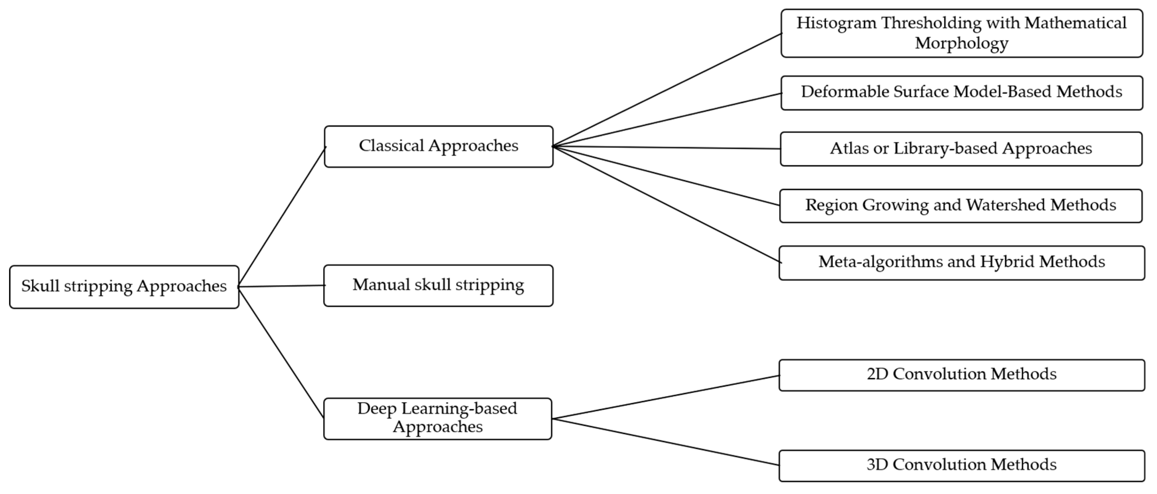
3. Classical or Conventional Skull Stripping Approaches

3.1. Histogram Thresholding with Mathematical Morphology

Thresholding with mathematical morphology-based algorithms utilizes thresholding using histogram analysis, edge detection, and a series of morphological operations—erosion, dilation, opening, closing, etc.—to isolate the brain and the non-brain regions. For instance, one of the most commonly used methods based on this technique was made by Brummer et al. [43]. It discriminates the skull from the brain by exploiting histogram thresholding followed by mathematical morphology filters. Atkins et al. [44] developed a multistage approach that utilizes anisotropic filters, histogram thresholding, a morphology filter, and snakes contouring techniques for segmenting the brain. Shan et al. [45] presented a similar histogram-based brain segmentation (HBRS) method based on histogram and morphological operations. Galdames et al. [46] proposed an automatic skull stripping method called SMHASS (simplex mesh and histogram analysis skull stripping) based on deformable models and histogram analysis. Initially, a rough segmentation step building on thresholds and morphological operations is used to find the optimal starting point for the deformation. The simplex mesh deformation is controlled by the local gray levels of the image and the information achieved on the gray level modeling of the rough segmentation.
The brain extraction algorithm (BEA) was developed by Somasundaram and Kalaiselvi [47,48] using diffusion, morphological operations, and connect component analysis (CCA) for T1W and T2W brain MRIs. Two-dimensional (2D) brain extraction was proposed by Gambino et al. [49] based on fuzzy c-means and morphological operations. The Brain Surface Extractor (BSE) is a well-known and publicly available tool for skull stripping devised by Shattuck et al. [50]. It employs the combination of anisotropic diffusion filtering, a Marr-Hildreth edge detector, and a series of morphological operations to identify the brain and non-brain regions. The BSE is extremely fast and generates highly explicit whole brain segmentation. It took only 3.5 (± 0.4) s for the whole brain extraction. BSE is also a part of BrainSuite [51] that affords a user interface that permits for human interface. The key deficiency of this technique is that it usually involves parameter tuning to work on a particular brain MRI dataset. The method based on grayscale transformation and morphological operations was presented by [52].
Similar to other approaches, the method devised by Sadananthan et al. [53] applies the grayscale level (or intensity) thresholding followed by the elimination of thin connections to acquire a fine brain mask. A graph cut technique was considered to smooth the contours of the brain instead of morphological filters. Balan et al. [54] proposed HEAD (human encephalon automatic delimiter), an automatic skull stripping method combining an efficient histogram analysis procedure and binary morphological operations to achieve accurate brain segmentation. Chiverton et al. [55] developed SMSS (the statistical morphology skull stripper), which employs statistical self-similarity and morphological operations to delineate the brain in an MRI. However, their algorithm produces skull stripping with minor amounts of over- and under-segmentation of the brain. Roy, S. et al. [56] introduced a robust skull stripping algorithm based on rough-fuzzy connectedness, termed ARoSi. Recently, Kavitha Srinivasan et al. [57] proposed an intelligent and robust mathematical morphology-based algorithm. The other latest methods include [58,59]. The major drawback of these approaches is that morphological operations depend on many fixed parameters, such as the shapes and sizes of structuring elements (for erosion, dilation, opening, etc.), which can only be found by empirical experimentation. For initial segmentation, the human (user) is normally involved in choosing the threshold value from a variety of starting thresholds. Another problem with these algorithms is that it is very hard to develop a general algorithm for diverse datasets of brain MRIs. It has proved challenging to automatically cope with a range of brain MRI resolutions and sequences [25]. In part, this is because it is very difficult to implement the problem-specific logical constraints (e.g., prior knowledge about brain MRIs, intensity/gray level, etc.) with these approaches.

3.2. Deformable Surface Model-Based Methods

Deformable surface model-based approaches normally evolve and deform a self-regulating dynamic curve (an active contour) to fit towards the brain surface based on the energy functions. Initially, a surface model is defined (e.g., a tessellated mesh of triangles) and then “fitted” to the surface of the brain in the image. Generally, there are two major parts of constraints to the fitting. The first part imposes some form of smoothness on the brain surface to keep it well-conditioned and match the actual smoothness value of the brain surface. The second part of constraints fits the model to the accurate region (or segments) of the brain surface. The fitting (sometimes referred to as curve evolution) is usually accomplished by iteratively deforming the active contour model from its starting position until an appropriate solution is achieved. These algorithms highly rely upon the initial position of the fitting curve and the image intensity variation (i.e., the image gradient). These parameters can betray the actual boundary of the brain and produce over/under the segmentation of the brain. For instance, Suri [60] utilized an active contour to segment the cerebrospinal fluid (CSF) and the white matter (WM) in brain MRIs using a fuzzy membership function, an image gradient detector, and a deformable model.
The algorithm brain extraction tool (BET), developed by Smith, S. M. [25], is the most prevalent and freely available algorithm of this category. In this method, the center of gravity and a rough brain/non-brain threshold of the brain MRI are found using a “robust” lower and upper grayscale values of the brain image. Then, it imposes locally adopted model forces to fit the surface of the brain employing a triangular tessellation of a sphere’s surface. This is also very fast and needs no preprocessing or other preregistration before being applied. BET was unsuccessful used to extract the brain region in the inferior brain slices (slices with the neck) when the center of gravity of the brain MRI volume lay outside the brain [61].
A new model-based level set (MLS) algorithm to separate intracranial tissues and the skull encircling the brain MRI was developed by Zhuang et al. [62]. The two terms (whose values represent the forces that influence the speed of the evolving curve) in the level set equation control the evolution of the curve. The first term was inferred from the mean curvature of the curve and the second was obtained from the intensity characteristics of the cortex in the brain MRIs. The combination of these two terms (forces) in the level set framework evolved the curve toward the brain surface. Liu et al. [63] presented a robust and automated brain extraction technique that utilizes an implicit deformable model to represent the contours of the brain and to segment the brain region. A set of Wendland’s radial basis functions (RBFs) described the model that has the advantages of low computational complexity and a compact support property. The contours of the brain are identified separately on 2D coronal and sagittal brain slices. The results from these two views are integrated to get a whole 3D brain MRI volume. A very recent article based on improved BET [25] was proposed by Wang et al. [64]. It evolves a 3D active mesh model to fit the brain surface in brain MRIs. A polygon fill algorithm has been used to generate a brain mask. Finally, a ray-casting volume rendering algorithm is utilized to visualize the brain surface from these generated brain masks.
One of the advantages associated with these techniques is that they can recognize both the exterior and interior boundaries of the brain simultaneously. Normally, deformable surface model-based approaches have the potential to achieve more precise and accurate skull stripping in brain MRIs than methods based on histogram thresholding, mathematical morphology, and edge detestation. However, these methods are highly susceptible to noise and fail to segment the brain in low contrast and noisy brain MRI datasets.

3.3. Atlas or Library-Based Methods

Atlas or library-based methods achieve brain labeling on the brain images using expert delineations of the brain MRIs. The labeled images subset is known as the atlas, training, or library set. These approaches rely on the target brain images being adequately analogous to the training set for the algorithm to transfer expert knowledge. Unlike other skull stripping methods, these algorithms often require significant preprocessing, such as intensity and spatial normalization [65]. These algorithms can isolate the brain from non-brain tissues when there is no well-defined relationship present between the respective brain region and the skull pixels’ intensities in the brain MRIs.
Dale et al. [66] designated a brain segmentation algorithm as a preprocessing step in the cortical surface reconstruction process by applying a tessellated ellipsoidal template. Leung et al. [67] proposed a template library-based segmentation technique called multiple-atlas propagation and segmentation (MAPS) that produces a segmentation of the brain utilizing a template library and non-linear atlas registration. It generates multiple segmentations from the best-matched templates with a manually segmented library and integrates them using an algorithm known as simultaneous truth and performance level estimation (STAPLE). The method has been developed and validated against manual measures employing subsets from the Alzheimer’s Disease Neuroimaging Initiative (ADNI). Leung et al. [68] also presented a method named “Brain MAPS” that compares the brain segmentation of the template library-based technique with BET [25], BSE [50], and HWA [69].
Similarly, Eskildsen et al. [70] developed BEaST, an automatic brain extraction technique, based on nonlocal segmentation incorporated in a multiresolution framework. Principally, this method is inspired by patch-based segmentation [71] where the sum of squared differences (SSD) has been exploited as the metric for the distance between patches. BEaST is much faster than the other label fusion methods and needed a smaller library of priors. Only a library of 50 priors was semi-automatically created from the data in the National Institutes of Health Pediatric Database (NIHPD) [72] the International Consortium for Brain Mapping (ICBM) database [73], and the Alzheimer’s Disease Neuroimaging Initiative (ADNI) [74]. The intensity and spatial normalization were performed before constructing the library of priors. The ground truth (or gold standard) of brain masks for library priors have been constructed using a semi-automatic method that includes manual correction. To enhance accuracy while reducing the computation time, an improved nonlocal label fusion scheme based on BEaST is proposed by Manjon et al. [75]. A new multi-atlas library construction pipeline has been introduced for better normalization between the template library subjects. The addition of bilateral patch similarity measure, a blockwise labeling approach, and a regularization constraint have aided the methods to increase accuracy and significant savings in computational cost.
Multi-atlas skull stripping has been presented in [76]. It is based on a multi-atlas registration framework to confront the challenges originating from the variability of imaging characteristics among different studies. After choosing a set of templates, they used a study-specific template selection strategy that best constitutes the anatomical variation within the dataset. To overcome the problems associated with the registration of brain images with the skull, an adapted registration algorithm was considered which adaptively aligned different regions of brains based on similarity and reliability of matching measures. In the last step, a spatially adaptive weighted voting strategy (ranking of Jacobian determinant values) has been used for joining the co-registered template masks.
Heckemann et al. [65] developed pincram, an automatic, versatile algorithm for accurately labeling 3D T1W brain MRIs in an adult. The algorithm applies an iterative refinement approach to transfer labels from multiple atlases to a specified target brain image utilizing image registration. A consensus label was generated at each refinement level of the algorithm. The search for brain boundary was confined to the neighborhood of the boundary of this consensus label at the successive level. This algorithm (Pincram) is also publicly available at [77] as free software.
Recently, a new multi-atlas brain segmentation (MABS) base brain masking technique was implemented by Del Re et al. [78]. In contrary to other atlas-based algorithms, MABS allows flexibility by assigning weights to the atlases with respect to their resemblance to the target image and circumvents the issue of atlas selection. The atlases most closely resembling the target image are given more weight in a set of heterogeneous atlases, than the atlases with less resemblance. Moreover, the MABS technique decreases the risk of averaging out individual differences by the inclusion of both pathological and control images in the training set. The authors also compare their results with FreeSurfer (FS; version 5.3) [39], BET [25], and Brainwash [79]. Ahmed Serag et al. [80] developed a novel method named ALFA (accurate learning with few atlases) for brain extraction of multimodal neonatal brain MRIs. The algorithm is combined with a new sparsity-based atlas selection strategy with a machine learning-based label fusion technique that requires a very limited number of atlases in low dimensional data space. Another recent method, “sparse patch-based multi-contrast brain stripping method (MONSTR),” published by Roy et al. [81] is also used non-local patch information from multiple atlases and integrate them to produce a final brain mask. This algorithm is also publicly available and insensitive to pathology. Other recent algorithms include [82].
The accuracy of Atlas or library-based Methods depends on the quality of brain masks, atlas registration, intensity and spatial normalization in each brain MRI volume. Furthermore, these approaches are generally computationally intensive.

3.4. Region Growing and Watershed Methods

Region growing (RG) and watershed methods inspect pixels in the brain MRIs and form separate connected regions based on a similarity criterion by merging neighborhood image pixels with uniformity properties. These methods start with at least one image pixel known as the seed that belongs to the region of interest (ROI). Seed neighbors’ pixels are examined against a similarity criterion that is defined prior to the start, and those neighbors’ pixels satisfying the criterion are included in the ROI (seed’s region). The criteria for similarity can be assessed and specified by intensity (or grayscale value) of the brain MRI pixels and other features in the brain image. Seed(s) can be (are) selected manually or by an automatic procedure based on the image’s properties (or prior knowledge). The RG process is repeated until a stopping criterion is reached. Hohne et al. [83] devised an interactive 3D segmentation of CT and brain MRI volumes based on RG and morphological filters. Justice et al. [84] are also proposed a 3D SRG (seeded region growing) method for brain MRI segmentation. Park and Lee [85] formulated an efficient and robust method based on 2-dimensional (2D) RG for brain T1W MRIs. In the first step, background voxels of brain MRI volume have been eliminated with histogram analysis. Next, seed regions, one for the brain and the other for the non-brain region, are identified utilizing a mask generated by morphological operations. Finally, the brain region is expanded by emerging neighborhood pixels of brain image with a 2D RG algorithm based on general brain structure information. This method can only be used for the coronal orientation of the brain MRIs. Roura et al. [86] eliminated this limitation and enabled their algorithm’s use in both axial views and low-quality brain images, and presented a new RG-based approach known as the multispectral adaptive region growing algorithm (MARGA) for skull stripping. It exploited the complementary information provided by brain MRIs and acquired a seed region that expanded using a 2D RG. Wang, L. et al. [87] developed a level set approach in a multistage formulation based on local Gaussian distribution fitting energy for brain extraction in MRI having intensity inhomogeneity. The intensities of the image are modeled by Gaussian distribution with various means and variances. Somasundaram et al. [48,88] proposed skull stripping techniques based on region labeling, clustering, and 2D RG. Hahn et al. [89] presented a simple and robust algorithm based on a modified 3D fast watershed transform to locate the brain tissues and remove the non-cerebral tissue in a T1W brain MRI. Segonne et al. [69] combined a deformable surface model [66] and the watershed algorithm [89] to form a new hybrid watershed algorithm (HWA) for brain segmentation. Sadananthan et al. [53] argued that the above two algorithms (Hahn et al. [89] and Segonne et al. [69]) diverge in their errors in the dissimilar region; thus, the intersection of the two algorithms would provide more robust skull stripping results.
The partial volume effect (PVE) [90] blurs and distorts the intensity distinctions between the various cerebral tissues of brain MRIs and confines the accuracy of the RG method. Furthermore, watershed algorithms typically suffer from over-segmentation of the brain tissue.

3.5. Meta-Algorithms and Hybrid Methods

An individual algorithm often will not sufficiently perform the whole brain extraction or skull stripping in every subject across an entire brain MRI dataset. Specifically, many different procedures must be tried or manual intervention utilized to attain satisfactory results. A simple way to access and test various approaches is an environment that presents many similar algorithms. A meta-algorithm or hybrid method that allows the requirement of a general procedure and achieves a valid result, regardless of input data, would permit the task of interpreting the results from many algorithms and selecting the best procedures to be fully automated. Each of the aforementioned skull stripping algorithms for brain MRIs possesses pros and cons that alter with the image characteristics; scanning protocol, such as image signal-to-noise ratio, contrast, and resolution; and subject-specific characteristics, such as age and atrophy [91,92]. Furthermore, the algorithms can also deviate in their accuracy in different brain anatomic regions [93]. The development of a hybrid algorithm that intelligently exploits the advantages of the contributing sub-algorithms should attain brain extraction results that are, typically, superior to any individual method.
Hybrid methods integrate the advantages of two or more approaches to enhance the precision and accuracy of skull stripping in brain MRIs. For example, Bauer et al. [94,95] combined atlas-based geodesic active contour brain segmentation with the level set-based algorithm and implemented it using the Insight Segmentation and Registration Toolkit (ITK) which they named “itk::StripTsImageFilter.” This hybrid algorithm successfully segments the brain in T1-contrast, T1W, and T2W-MRIs; computed tomography (CT); and FLAIR images. David E. Rex et al. [96] developed the brain extraction meta-algorithm (BEMA) by executing four different brain extractors (including BSE [50], BET [25], 3dIntracrnial [97], and Watershed from FreeSurfer [66]) and a registration procedure in parallel to integrate the brain extraction results in an intelligent way and achieve improved results over any of the individual algorithms. The algorithm performs a voxel-wise analysis of training data to find the optimal Boolean grouping of extraction algorithms to generate the most precise segmentation results for a given voxel.
Segonne et al. [69] combined a deformable surface model [66] and the watershed algorithm [89] to form a new hybrid watershed algorithm (HWA) for brain segmentation. The deformable surface model effectively incorporates the geometric information of the brain MRI but cannot have access to the intensity information of the interior region of the brain. Similarly, watershed algorithms ignore the geometric information. By combining both approaches, their hybrid algorithm obtained improved results over either one individually. Another hybrid method based on the expectation-maximization algorithm, mathematical morphology, connected component analysis, and geodesic active contours was presented by Huang et al. [98]. A well-known learning-based algorithm “robust brain extraction (ROBEX)” was presented by Iglesias et al. [99]. It incorporates a discriminative (random forest) and a generative model (point distribution) with the graph cuts for whole-brain extraction. The brain boundary is identified using a random forest (RF) classifier. A triangular mesh, constrained by a point distribution model, is evolved to fit the probabilistic output of RF. The deformation (contour) is refined and optimized using graph cut. It exhibited improved performance without any parameter settings. ROBEX is publicly available as the ”ROBEX1.2” package available at [100].
William Speier et al. [101] extend the ROBEX skull stripping method and presented a technique to extract the brain from glioblastoma multiform (GBM) images. They trained a shape model on healthy brain MRIs which is relatively insensitive to lesions inside the brain. Adaptive thresholding has been employed to search for potential resection cavities at the brain boundary, and random walker (RW) [102] corrects for a leakage into ventricles. Another efficient algorithm formulated by Aaron et al. [103] is known as the “simple paradigm for extra-cerebral tissue removal (SPECTRE)”; it is for skull stripping. It integrates different techniques, such as elastic registration, bran tissue segmentation, and morphological operations directed by the watershed principle. Primarily, SPECTRE was designed for T1W brain MRIs. However, the authors mentioned that it can be employed with other modalities (e.g., T2W and PDW) with a simple alteration. Shi et al. [104] proposed a novel meta-algorithm, “brain extraction and labelling (LABEL),” for skull stripping, especially for pediatric brain MRIs. Other recent and new skull stripping methods are [105,106]. One of the disadvantages of meta-algorithms and hybrid methods is that they often demand extensive training of the data to learn the particular brain features to accurately segment the brain MRIs.
Some well-known conventional skull stripping algorithms have been listed in Table 3.

4. CNN-Based or Deep Learning-Based Approaches

Brian MRIs can be captured at different angles, and under different magnetic strength conditions. Therefore, the image parameters contain a lot of very diverse information. Consequently, robustness to these changes is very crucial in the development of algorithms. In general, deep learning-based skull stripping approaches are divided into two distinct groups: 2D skull-stripping methods and 3D skull-stripping methods. Although 3D skull-stripping is thought to produce better results because contextual information between adjacent slices can be additionally used, it is computationally very expensive, so 2D skull-stripping has been more commonly adopted than the 3D method. 2D skull-stripping methods are categorized into two groups. The first group contains a voxel-wise neural network and the second group comprises fully connected CNNs. The networks of the first group predict the class of a voxel from multiple image patches, whose center the voxel is located using multiple 2D CNNs and a fully connected network. The networks of the second group adopt an encoder-decoder structure. The encoder part reduces the size of the image simultaneously extracting features, and the decoder expands the image in order to get high resolution segmentation results. One of the most used networks in medical image segmentation, U-Net [108], employes this encoder-decoder structure. Generally, the second group’s methods are more efficient than the first ones because fully convolutional networks can recognize both local and global features. Moreover, the first group’s methods have the disadvantage that the size of the input image is fixed, but fully convolutional networks are not limited to this condition and are also fast.

4.1. 2D Skull-Stripping Method

2D semantic segmentation predicts the total volume by segmenting each slice independently and by combining the results of 2D segmentation. Generally, 2D semantic segmentation is faster than 3D segmentation and there are many techniques for it compared to 3D semantic segmentation. Because it is based on the 2D slice as input, it does not take advantage of the context of adjacent slices. In order to overcome this limitation, 2D skull-stripping methods making use of adjacent information have been introduced and some of them showed similar performances to the 3D based methods with less computation.
Salehi et al. [109] proposed two methods: a voxel-wise network and a fully convolutional network. The first is a parallel voxel-wise network and the second is a parallel 2D FCN U-Net. Each network is followed by an auto-context CNN classifier. It was named Auto-Net. The authors pointed out that the biggest problem with 3D CNN is its expensive computation and proposed to use two networks. The first network consists of three 2D networks (axial, coronal, and sagittal) instead of the computationally expensive 3D CNN. The 2D network receives the input image in three different sized patches. The reason for using three different patches is to get both local and global information. This network has much reduced the number of parameters compared to 3D CNN while showing as good a performance as 3D CNN does. The second proposed network is a fully convolutional network based on U-Net [108]. It integrates the contextual information by combining the low-level appearance feature and the high-level appearance feature from an auto-context algorithm. Auto-Net needs a trained model in each plane to utilize auto-context, so it is not an end-to-end form.
Lucena et al. [110] proposed a network consisting of two main parts. The first part is a network having three 2D CNNs, and the second part is a network handling context variation. The three 2D CNNs handle three planes of space (axial, coronal, and sagittal). The authors call this CONSNet. The authors showed a better performance than the one-way process by adopting this tri-planar approach. 3D segmentation is achieved by reconstruction of the output of 2D prediction through concatenation. Interestingly, the authors used so-called silver standard masks instead of gold-standard masks as ground truth. Silver standard masks mean the labels created through consensus that are the results of publicly available non-deep learning-based skull-stripping methods. Gold standard masks are manual masks created by experts. In the paper, the authors reported that the proposed method outperformed in the LPBA40 and OASIS datasets, despite training with only the CC-359 dataset. Using silver-standards is a big advantage because it significantly reduces the cost of manual annotation. Silver-standards masks were obtained by forming a consensus from eight automated skull-stripping methods. Lucena et al. [111] also published papers using 2D FCN U-Net. The authors used silver standard masks to train the model and claimed that it showed comparable generalization performance when compared to gold standard masks. Furthermore, the results show that silver standard masks can be used to augment the data to reduce the need for manual segmentation. Inspired by this paper, Carmo et al. [112] performed hippocampus segmentation on three planes using 2D FCN U-Net. However, they have proposed a better way than adding additional networks to get a final consensus. They added the activation heatmap to each 2D FCN U-Net, applied a predefined threshold, and performed 3D labeling. This method showed much better performance than that of Lucena et al. [111].
Yilmaz et al. [113] performed skull stripping using a cellular neural network called the multistable cellular neural network on MRI for skull stripping (mCNN-MRI-SS). They proposed using contrast enhancement for preprocessing by a linear image combinations algorithm. This leads to less noise and improved contrast results. The parameter determination for all training is done by the artificial bee colony (ABC) algorithm. The ABC algorithm is an optimization algorithm based on swarm intelligence. They mentioned that the solution of coefficient parameters, templates, and output functions requires a large multidimensional search space, so the authors proposed using the ABC algorithm because it has a wide search space. The mCNN-MRI-SS algorithm shows similar or worse performance than BET and BSE, especially on superior and inferior slices. This may be due to calculation errors in the analysis process. The calculation speed is also slow compared to other algorithms since the analysis algorithm is applied to all particles.
The next paper proposed skull stripping using a confidence segmentation convolutional neural network (CSCNet) [114]. CSCNet adopted an encoder-decoder structure. The network is very similar to SegNet [115], one of the most frequently used networks in semantic segmentation. The only difference is that while the authors of SegNet adhered to use the activation function as a softmax function, the author used the ReLU function. This ReLU function is used to produce a confidence level in the pixels of the image. Using the fact that MR images are grayscale, the author created a confidence level matrix as a bitmask and applied it to the original. The reason is that the author’s model cannot output accurate brain tissue, so they use the results of the activation function trained based on the target image. In other words, the higher the activated state, the higher the reliability. CSCNet performs better than the other methods, but it is not robust with respect to artifacts.
Duy et al. [116] presented a method that combines both the advantages of the active shape model (ASM) and CNN. ASM [117] is a statistical model that finds the desired object through an iterative transformation of data to find the desired object in a new image. ASM is widely used in face image analysis and medical imaging. To proceed with the ASM, the shape of the object should be searched and attribute information indicated by each feature point of the object is required. There are some points worth mentioning in this paper. First, instead of dealing with 3D structures, the brain image is regarded as a continuous form of the sagittal planes which are symmetrical. It allows making more sophisticated segmentation by predicting the second half with data from the first half. The brain is divided into three groups according to the criteria set by the authors. The first group is the smallest but has a very complicated structure, and the third group is the largest. In each group, slices have a very similar form. Having a similar form allows the algorithm to achieve high accuracy segmentation. Second, ASM is used to find the brain boundaries of the image using the prior information of each group. ASM is applied in the second and third groups first. The contour generated from ASM is refined using post-processing techniques, such as a CNN, a conditional random field, and a Gaussian process, and some special other rules. Next, segmentation results of the second group are fed to CNN that processes the first group, making it easier to deal with the first group that is difficult to process. The ASM algorithm, however, only works well when the shape of the test image is similar to the shape of the training image.
The skull and the brain look very similar in MRI images, so it is difficult to differentiate them. To solve this problem, Dey et al. [118] created a CompNet network using creative ideas. The network employed encoder-decoder networks. It has two pathways, the first path learning the features of the brain tissue and the second path learning the complementary part located outside the brain. This technique provides a robust solution for brain extraction from MRIs. However, due to the lack of true masks for complementary parts, the authors created a sub-encoder-decoder network that reconstructs the original one based on the output of the two branches. Sub-encoder-decoder networks provide direct feedback to networks processing brain parts and complementary parts to reconstruct the original one. Optimal CompNet shows higher accuracy when compared with one of the most popular networks such as U-Net and dense U-Net.
NeuroNet [119] is a network that mimics state-of-the-art brain segmentation tools such as FSL [120], SPM [121], and others [122]. The network was trained from 5000 T1-weighted brain MRI scans that were automatically segmented from standard neuroimaging pipelines (FSL, SPM, and others). The structure of the network is as follows. There is one encoder structure and multiple decoders that receive the output of the encoder and extract the final result. Each decoder teaches the state-of-the-art brain segmentation tool. Generating multiple outputs from a single model can be very powerful due to overlapping label maps. Besides, it is very efficient because it outputs several results at once. The authors also asserted that networks are very robust from changes in input data. Another advantage is that Neuronet does not require typical preprocessing. In other words, the network can produce output from raw images and no additional hyper-parameters are required.
Next, we briefly introduce the deep learning techniques that are widely used as general 2D semantic segmentation and therefore can be applicable to the skull-stripping problem. Fully Convolutional networks for semantic segmentation (FCN) [123] showed high improvements in the field of semantic segmentation. What differentiates FCN from previous semantic segmentation papers is that the fully connected layer is removed. Existing papers had the problem that the location information was removed through the fully connected layer. Therefore, the authors of FCN replaced the fully connected layer with a 1 × 1 convolution. Next, upsampling was performed to restore the original size of the image. Instead of performing interpolation, the output from the encoder is combined after interpolation to obtain the result of segmentation in detail. SegNet [115] came out in 2015. This network is similar to FCN in that it uses encoder-decoder architectures. However, the key difference is that more shortcut connections are used, and instead of copying encoder functionality as in FCN, Maxpooling’s indices are transitioned to increase memory efficiency.
U-Net [108] also forms a structure similar to the previous FCN and SegNet. U-Net is divided into contracting path and expanding path. The contracting path is used to identify the global context and the expanding path is used to identify the local details. The key point of U-Net is that it allows for more accurate localization by concatenating the output of the contracting path prior to each upconvolution of the expanding path. As a way to solve the semantic segmentation problem, the key point of DeepLab is using atrous convolution. DeepLab V1 [124] first applied atrous convolution for semantic segmentation. Atrous convolution is the novel method which makes the stride between elements of a convolution filter. As the distance gets longer, the filter can cover a wider field of view with the same number of parameters. In general, since the size of the receptive field determines the performance of semantic segmentation, it is a big advantage to have a wide receptive field without increasing the amount of computation.
DeepLab V2 [125] proposed the atrous spatial pyramid pooling (ASPP) technique for applying multiscale contexts. The technique performs atrous convolution over various distances and then concatenates the results. This technique allows for identifying all local and global features, making it possible to identify multiscale contexts accurately. DeepLab V3 [126] proposed a more dense feature map by using an atrous convolution in existing ResNet structures. DeepLab V3+ [127] proposed the use of atrous separable convolution, which combines separable convolution and atrous convolution. The decoder part which was taken simply by bilinear upsampling, was replaced with a decoder similar to U-Net. As a result, separable convolution was utilized to maximize the performance in the encoder, ASPP, and decoder. At the end of 2016, RefineNet [128] was submitted to Arxiv. RefineNet pointed out the limitations of dilated/atrous convolutions and suggested using existing encoder and decoder networks. Before putting the result of the encoder into the decoder, the RefineNet block combines multiresolution features by upsampling low-resolution features. This allows capturing contextual information. The average precision of different deep learning algorithms can be seen on voc2012 [129] dataset.

4.2. 3D Skull-Stripping Method

Unlike the 2D skull-stripping method, which does not utilize the context of adjacent slices, the 3D skull-stripping method can utilize all three-dimensional information, leading to better segmentation results. However, it has the disadvantage of using a large amount of computation. Kleesiek et al. [130] proposed the network structure which consists of seven 3D convolutional hidden layers and one convolutional soft-max output-layer. The network was specially designed only for skull stripping. The authors wanted to cover brains of various ages, brains with artifacts, and brains of various shapes with minimal parameter tuning. Furthermore, the goal was to create a robust network for any single modality or the combination of several modalities (T1W, T2 W, T2-FLAIR, etc.). The author tested different structures by adding and removing various layers and found that the proposed structure shows the best performance. When compared with the most popular conventional methods (BET, BSE, Robex, etc.) on IBSR [41], LPBA40 [40], and OASIS [36] datasets, Kleesiek’s [130] method showed the highest performance in terms of dice and specificity but average performance in sensitivity.
Hwang et al. [93] suggested that 3D-UNet, the general 3D segmentation network, could be used for skull-stripping problems. The authors showed that the performance is comparable to the method developed by Kleesiek et al. [130]. The test result of the NFBS dataset showed that Kleesiek et al.’s network has better performance in terms of dice and specificity and 3D-UNet shows better performance regarding sensitivity.
Huo et al. [131] showed a technique that improves the performance by using both the classic method and the deep learning method together. The authors point out that the network has limitations because it learns spatial and contextual information from numerous image patches, and the number of medical images is too small to train the network. To solve those two problems, the author proposed the spatially localized atlas network tiles (SLANT) method. Multiple spatially distributed networks were used to overcome the spatial limitation. Each network was trained from fixed patches. Since multiple networks are used, each network can focus on finding the differences from very similar patches. To enable this strategy, affine registration and intensity normalization were used in advance. Finally, label fusion was used to produce the result from the network tiles. To increase the number of training image sets, the authors made auxiliary labels from 5111 unlabeled scans. The auxiliary labels were made through multi-atlas segmentation. However, the biggest problem with the method is that it requires a lot of computational resources. If only one GPU is used, the training time or the test time increases linearly whenever the network tile increases.
Isensee et al. [132] created their own network based on U-Net but upgraded its structure. The authors attempted to create a network that is robust to the deformation of the brain tissue by disease or treatment and is not affected by the deformation of MRI hardware. Their modification is as follows: First, preactivation residual blocks were put in the encoder section of U-Net, and the results of the block were concatenated with the original one. It deepens the network architecture and improves gradient flow. The patch size was 128 × 128 × 128 voxels and the voxel resolution was 1.5 × 1.5 × 1.5 mm 3 . It almost covers the entire brain. The large patch size allows the brain mask to be accurately reconstructed, although any part of the brain can be lost due to an accident. Second, they created auxiliary loss layers. The gradients in the deep part of U-Net are very small due to chain rules, making it very difficult to train deep parts. Thus, the authors tried to solve this problem by putting auxiliary loss layers into the deep part. Finally, the authors changed the activation function and the normalization function. The authors found the ReLU function dying in the deep networks, so they replaced it with the leakyReLU function. In the proposed method, the batch size is smaller than other methods. Therefore, the batch means and the standard deviation are unstable. For this reason, the authors applied instance normalization instead of batch normalization. Instance normalization is that each batch normalizes independently from the other batch. Although Isensee’s method was applied to brains with tumors or normal brains, their HD-BET algorithm is expected to also work in a wide range of diseases in neuroradiology.
Fedorov et al. [133] introduced a deep learning model based on volumetric dilated convolutions. Dilated convolutions is another name for atrous convolutions introduced by Deeplab [124]. Compared to other models, this model significantly reduced the number of parameters, shortening the processing time and showing high accuracy for test data. Another important characteristic of this model was that it showed high accuracy even when trained on imperfect data.
FRnet [134] offers novel methodologies in three ways. First, the authors created it based on U-Net. The difference between FRnet and U-Net is that it executes residual block after a “de-convolution + batch normalization + ReLU” block in the decoder part. It is also novel to apply convolution before concatenation. Another difference is that a new loss function was used to highlight the boundary regions that are ambiguous and blurry. The loss function is weighted at the boundary region since the boundary is always the most important part of the segmentation map.
Finally, Beers et al. [23] introduced a deep learning framework that puts the best fit deep learning algorithms in order to deal with neuroimaging practically. The authors noted that many packages are very good at sharing and designing deep learning algorithms, but few provide utilities for working with clinical data. The authors showed how the framework designs and trains the network, and how to modify the state-of-the-art architecture in a flexible and intuitive way using their toolbox. In addition, by providing preprocessing and post-processing which are frequently used in medical imaging, the framework has shown a consistent performance in various environments. Once the author develops a GUI interface for users with no coding capability, it is expected to be more helpful. Table 4 summarizes deep learning-based methods that have been described in the preceding sections.
In the next part, we briefly introduce deep learning-based techniques that have been recently proposed for 3D semantic segmentation, and are applicable to our 3D skull-stripping problem. The first network is 3D U-Net [135]. This network is based on a model created by extending one dimension on the existing 2D U-Net. Not only were the methods used in 2D U-Net used for 3D, but they also added techniques such as batch normalization [136]. The strength of this network is that it can learn from sparsely annotated volumetric images. Similar to 3D U-Net, V-Net [137] is a network that has end-to-end structures. It is composed of encoder and decoder. The existing networks generally downsample and upsample using pooling, while V-Net downsamples and upsamples using convolution layers with strides. VoxResNet [138] consists of 25 layers, including the VoxRes module. The VoxRes module corresponds to ResNet’s [139] residual unit in three dimensions. Here, the deconvolution of the output of every fourth block is performed to classify and merge the result to get the final output. The advantage of this approach is the integration of multimodality and multilevel contextual information. As a result, the overall information can be learned and the functions of various scales can be utilized, resulting in increased segmentation performance. DenseVoxNet [140] was proposed. This network outperforms 3D U-Net and VoxResNet even with fewer parameters. Similar to VoxResNet, the network consists of a DenseBlock, which extends the dense connections of DenseNet [141] in three dimensions. The benefits of DenseBlock include less information loss, a lesser gradient vanishing problem, and fewer learning parameters.
Although deep learning-based methods revolutionized image segmentation by automatically learning the most difficult feature representations from data, they still have drawbacks. One of the major drawbacks of deep learning methods is the inability to show how to get the result. Deep learning models are basically black boxes. This opacity of deep learning makes deep learning difficult to understand or difficult to improve. As a result, developers do not know how to adjust the numerous hyperparameters of a deep learning model and how to improve the performance of the model. Unfortunately in many cases, they have no choice but to rely on trial and error, which are very inefficient. Another problem is the limitation of data-dependence. Basically, a lot of data is needed to properly train a deep learning network model. This is a well-known characteristic of deep learning methods. For this purpose, various open databases for general images have been built and keep accumulating data. However, this is not a simple problem for medical imaging, because collecting lots of annotated datasets in medical images is often very difficult, time-consuming, and expensive, not to mention the ethical concerns and privacy issues. Global collaboration is the only way to address this data issue wisely and effectively.
Finally, Table 5 summaries publicly available packages with their respective online links. Users can download and execute their packages from the links. The upper part of the table shows links of conventional methods, and the lower part of the table shows links of deep learning methods.

5. Conclusions

This review article has presented a comprehensive and extensive overview of the state-of-the-art conventional and CNN deep learning-based skull stripping (or whole-brain extraction) methods in brain MRIs. Many of the available approaches employed mainly T1W brain MRIs due to good soft-tissue contrast. Even though most of the published algorithms have relatively decent results in the field of neuroimage analysis, there is a certain distance and discontinuity between the research community and clinical applications. In most cases, clinicians and practitioners still depend on manual skull stripping due to the communication gap and lack of interaction between the researchers and practitioners. The objective of several skull stripping tools is to do only the research, and they are barely useful for clinicians. Therefore, embedding the developed tools into more user-friendly environments will become inevitable in the future. Consequently, incorporating all the accessible developed skull stripping into a more intelligible and easier-to-use environment will become unavoidable in the future. Although deep learning-based methods have attained exceptional performance in skull stripping, the computation time is unsatisfactory in a clinical routine, as these approaches can take a few minutes per volume of brain MRI. Time is also an important criterion for real neuroimaging applications. Another critical issue for skull stripping in brain MRI approaches is robustness. If an automatic brain extraction technique is unsuccessful in some cases, the trust of clinicians will be lost, and they will stop using this method. Hence, the robustness is also one of the keys and foremost evaluation criteria for each new algorithm applied in clinical practice. Optimization of the skull stripping methods, particularly those CNN deep learning-based, to make them faster, is also future work. However, some current skull stripping methods have presented robust results within an acceptable computation time.
The existing brain extraction techniques have already demonstrated great potential in skull stripping in T1W brain MRIs and will certainly continue to be improved in the future. Furthermore, widely published algorithms mostly considered normal healthy subjects brain MRIs except a few (e.g., Roy et al. [81], and Lutkenhoff et al. [107]). They started deterioration in their performance and become less accurate when presented with brain MRIs having pathologies. There is a need for modification in the existing techniques or developing new algorithms for other modalities, such as T2W, T2W FLAIR, PDW, and brain MRIs with lesions or pathologies. This provides more room and predictive medical information to the practitioner and optimizes treatment options.

Author Contributions

S.L. proposed the idea; H.Z.U.R. and H.H. contributed to writing the manuscript. S.L. supervised the study and the manuscript-writing process, and made suggestions for manuscript correction and improvements. All authors have read and agreed to the published version of the manuscript.

Funding

This work was in part supported by the convergence technology development program for bionic arm through the National Research Foundation of Korea (NRF) funded by the Ministry of Science and ICT (number 2015M3C1B2052811), Republic of Korea. This work was also supported by the Technology Innovation Program (or Industrial Strategic Technology Development Program) (20001856, Development of robotic work control technology capable of grasping and manipulating various objects in everyday life environment based on multimodal recognition and using tools) funded by the Ministry of Trade, Industry and Energy (MOTIE), Republic of Korea.

Conflicts of Interest

The authors declare no conflict of interest.

References

  1. Sugimori, H.; Kawakami, M. Automatic Detection of a Standard Line for Brain Magnetic Resonance Imaging Using Deep Learning. Appl. Sci. 2019, 9, 3849. [Google Scholar] [CrossRef] [Green Version]
  2. Du, X.; He, Y. Gradient-Guided Convolutional Neural Network for MRI Image Super-Resolution. Appl. Sci. 2019, 9, 4874. [Google Scholar] [CrossRef] [Green Version]
  3. Kapellou, O.; Counsell, S.J.; Kennea, N.; Dyet, L.; Saeed, N.; Stark, J.; Maalouf, E.; Duggan, P.; Ajayi-Obe, M.; Hajnal, J.; et al. Abnormal Cortical Development after Premature Birth Shown by Altered Allometric Scaling of Brain Growth. PLoS Med. 2006, 3, e265. [Google Scholar] [CrossRef] [PubMed] [Green Version]
  4. Boardman, J.P.; Walley, A.; Ball, G.; Takousis, P.; Krishnan, M.L.; Hughes-Carre, L.; Aljabar, P.; Serag, A.; King, C.; Merchant, N.; et al. Common genetic variants and risk of brain injury after preterm birth. Pediatrics 2014, 133, e1655–e1663. [Google Scholar] [CrossRef] [PubMed]
  5. Porter, E.J.; Counsell, S.J.; Edwards, A.D.; Allsop, J.; Azzopardi, D. Tract-Based Spatial Statistics of Magnetic Resonance Images to Assess Disease and Treatment Effects in Perinatal Asphyxial Encephalopathy. Pediatric Res. 2010, 68, 205–209. [Google Scholar] [CrossRef] [Green Version]
  6. Kwon, S.H.; Vasung, L.; Ment, L.R.; Huppi, P.S. The Role of Neuroimaging in Predicting Neurodevelopmental Outcomes of Preterm Neonates. Clin. Perinatol. 2014, 41, 257–283. [Google Scholar] [CrossRef]
  7. Bauer, S.; Wiest, R.; Nolte, L.-P.; Reyes, M. A survey of MRI-based medical image analysis for brain tumor studies. Phys. Med. Biol. 2013, 58, 97. [Google Scholar] [CrossRef]
  8. Uhlich, M.; Greiner, R.; Hoehn, B.; Woghiren, M.; Diaz, I.; Ivanova, T.; Murtha, A. Improved Brain Tumor Segmentation via Registration-Based Brain Extraction. Forecasting 2018, 1, 59–69. [Google Scholar] [CrossRef] [Green Version]
  9. Makropoulos, A.; Gousias, I.S.; Ledig, C.; Aljabar, P.; Serag, A.; Hajnal, J.V.; Edwards, A.D.; Counsell, S.J.; Rueckert, D. Automatic Whole Brain MRI Segmentation of the Developing Neonatal Brain. IEEE Trans. Med Imaging 2014, 33, 1818–1831. [Google Scholar] [CrossRef]
  10. Cardoso, M.J.; Melbourne, A.; Kendall, G.S.; Modat, M.; Robertson, N.J.; Marlow, N.; Ourselin, S. AdaPT: An adaptive preterm segmentation algorithm for neonatal brain MRI. Neuroimage 2013, 65, 97–108. [Google Scholar] [CrossRef]
  11. Li, G.; Wang, L.; Shi, F.; Lyall, A.E.; Lin, W.; Gilmore, J.H.; Shen, D. Mapping Longitudinal Development of Local Cortical Gyrification in Infants from Birth to 2 Years of Age. J. Neurosci. 2014, 34, 4228–4238. [Google Scholar] [CrossRef] [PubMed] [Green Version]
  12. Zhou, F.; Zhuang, Y.; Gong, H.; Zhan, J.; Grossman, M.; Wang, Z. Resting State Brain Entropy Alterations in Relapsing Remitting Multiple Sclerosis. PLoS ONE 2016, 11, e0146080. [Google Scholar] [CrossRef] [PubMed]
  13. Sowell, E.R.; Trauner, D.A.; Gamst, A.; Jernigan, T.L. Development of cortical and subcortical brain structures in childhood and adolescence: A structural MRI study. Dev. Med. Child Neurol. 2002, 44, 4–16. [Google Scholar] [CrossRef] [PubMed] [Green Version]
  14. Tanskanen, P.; Veijola, J.M.; Piippo, U.K.; Haapea, M.; Miettunen, J.A.; Pyhtinen, J.; Bullmore, E.T.; Jones, P.B.; Isohanni, M.K. Hippocampus and amygdala volumes in schizophrenia and other psychoses in the Northern Finland 1966 birth cohort. Schizophr. Res. 2005, 75, 283–294. [Google Scholar] [CrossRef] [PubMed]
  15. Leote, J.; Nunes, R.G.; Cerqueira, L.; Loução, R.; Ferreira, H.A. Reconstruction of white matter fibre tracts using diffusion kurtosis tensor imaging at 1.5T: Pre-surgical planning in patients with gliomas. Eur. J. Radiol. Open 2018, 5, 20–23. [Google Scholar] [CrossRef] [Green Version]
  16. Tosun, D.; Rettmann, M.E.; Naiman, D.Q.; Resnick, S.M.; Kraut, M.A.; Prince, J.L. Cortical reconstruction using implicit surface evolution: Accuracy and precision analysis. Neuroimage 2006, 29, 838–852. [Google Scholar] [CrossRef] [Green Version]
  17. Fein, G.; Landman, B.; Tran, H.; Barakos, J.; Moon, K.; Di Sclafani, V.; Shumway, R. Statistical parametric mapping of brain morphology: Sensitivity is dramatically increased by using brain-extracted images as inputs. Neuroimage 2006, 30, 1187–1195. [Google Scholar] [CrossRef] [Green Version]
  18. Acosta-Cabronero, J.; Williams, G.B.; Pereira, J.M.; Pengas, G.; Nestor, P.J. The impact of skull-stripping and radio-frequency bias correction on grey-matter segmentation for voxel-based morphometry. Neuroimage 2008, 39, 1654–1665. [Google Scholar] [CrossRef]
  19. Fischmeister, F.P.; Hollinger, I.; Klinger, N.; Geissler, A.; Wurnig, M.C.; Matt, E.; Rath, J.; Robinson, S.D.; Trattnig, S.; Beisteiner, R. The benefits of skull stripping in the normalization of clinical fMRI data. Neuroimage Clin. 2013, 3, 369–380. [Google Scholar] [CrossRef] [Green Version]
  20. Smith, S.M.; De Stefano, N.; Jenkinson, M.; Matthews, P.M. Normalized accurate measurement of longitudinal brain change. J. Comput. Assist. Tomogr. 2001, 25, 466–475. [Google Scholar] [CrossRef] [Green Version]
  21. Smith, S.M.; Rao, A.; De Stefano, N.; Jenkinson, M.; Schott, J.M.; Matthews, P.M.; Fox, N.C. Longitudinal and cross-sectional analysis of atrophy in Alzheimer’s disease: Cross-validation of BSI, SIENA and SIENAX. Neuroimage 2007, 36, 1200–1206. [Google Scholar] [CrossRef] [PubMed]
  22. Souza, R.; Lucena, O.; Garrafa, J.; Gobbi, D.; Saluzzi, M.; Appenzeller, S.; Rittner, L.; Frayne, R.; Lotufo, R. An open, multi-vendor, multi-field-strength brain MR dataset and analysis of publicly available skull stripping methods agreement. Neuroimage 2018, 170, 482–494. [Google Scholar] [CrossRef] [PubMed]
  23. Beers, A.; Brown, J.; Chang, K.; Hoebel, K.; Gerstner, E.; Rosen, B.; Kalpathy-Cramer, J. DeepNeuro: An open-source deep learning toolbox for neuroimaging. arXiv 2018, arXiv:1808.04589. [Google Scholar]
  24. Puccio, B.; Pooley, J.P.; Pellman, J.S.; Taverna, E.C.; Craddock, R.C.J.G. The preprocessed connectomes project repository of manually corrected skull-stripped T1-weighted anatomical MRI data. Gigascience 2016, 5, 45. [Google Scholar] [CrossRef] [Green Version]
  25. Smith, S.M. Fast robust automated brain extraction. Human Brain Mapp. 2002, 17, 143–155. [Google Scholar] [CrossRef]
  26. Jin, L.; Min, L.; Wang, J.; Fangxiang, W.; Liu, T.; Yi, P. A survey of MRI-based brain tumor segmentation methods. Tsinghua Sci. Technol. 2014, 19, 578–595. [Google Scholar] [CrossRef]
  27. Kalavathi, P.; Prasath, V.S. Methods on skull stripping of MRI head scan images—A review. J. Digit. Imaging 2016, 29, 365–379. [Google Scholar] [CrossRef] [Green Version]
  28. Litjens, G.; Kooi, T.; Bejnordi, B.E.; Setio, A.A.A.; Ciompi, F.; Ghafoorian, M.; van der Laak, J.; van Ginneken, B.; Sanchez, C.I. A survey on deep learning in medical image analysis. Med. Image Anal. 2017, 42, 60–88. [Google Scholar] [CrossRef] [Green Version]
  29. Krizhevsky, A.; Sutskever, I.; Hinton, G.E. ImageNet classification with deep convolutional neural networks. In Proceedings of the 25th International Conference on Neural Information Processing Systems, Lake Tahoe, NV, USA, 3–8 December 2012; Volume 1, pp. 1097–1105. [Google Scholar]
  30. LeCun, Y.; Bengio, Y.; Hinton, G. Deep learning. Nature 2015, 521, 436–444. [Google Scholar] [CrossRef]
  31. Greenspan, H.; van Ginneken, B.; Summers, R.M. Guest Editorial Deep Learning in Medical Imaging: Overview and Future Promise of an Exciting New Technique. IEEE Trans. Med Imaging 2016, 35, 1153–1159. [Google Scholar] [CrossRef]
  32. Weiner, M.W.; Aisen, P.S.; Jack, C.R., Jr.; Jagust, W.J.; Trojanowski, J.Q.; Shaw, L.; Saykin, A.J.; Morris, J.C.; Cairns, N.; Beckett, L.A.; et al. The Alzheimer’s disease neuroimaging initiative: Progress report and future plans. Alzheimers Dement. 2010, 6, 202–211. [Google Scholar] [CrossRef] [PubMed] [Green Version]
  33. Weiner, M.W.; Veitch, D.P.; Aisen, P.S.; Beckett, L.A.; Cairns, N.J.; Cedarbaum, J.; Donohue, M.C.; Green, R.C.; Harvey, D.; Jack, C.R., Jr.; et al. Impact of the Alzheimer’s disease neuroimaging initiative, 2004 to 2014. Alzheimers Dement. 2015, 11, 865–884. [Google Scholar] [CrossRef] [PubMed] [Green Version]
  34. Weiner, M.W.; Veitch, D.P.; Aisen, P.S.; Beckett, L.A.; Cairns, N.J.; Green, R.C.; Harvey, D.; Jack, C.R.; Jagust, W.; Liu, E.; et al. The Alzheimer’s Disease Neuroimaging Initiative: A review of papers published since its inception. Alzheimers Dement. 2013, 9, e111–e194. [Google Scholar] [CrossRef] [PubMed] [Green Version]
  35. Weiner, M.W.; Veitch, D.P.; Aisen, P.S.; Beckett, L.A.; Cairns, N.J.; Green, R.C.; Harvey, D.; Jack, C.R., Jr.; Jagust, W.; Morris, J.C.; et al. The Alzheimer’s Disease Neuroimaging Initiative 3: Continued innovation for clinical trial improvement. Alzheimers Dement. 2017, 13, 561–571. [Google Scholar] [CrossRef] [PubMed] [Green Version]
  36. Marcus, D.S.; Wang, T.H.; Parker, J.; Csernansky, J.G.; Morris, J.C.; Buckner, R.L. Open Access Series of Imaging Studies (OASIS): Cross-sectional MRI data in young, middle aged, nondemented, and demented older adults. J. Cogn. Neurosci. 2007, 19, 1498–1507. [Google Scholar] [CrossRef] [PubMed] [Green Version]
  37. Marcus, D.S.; Fotenos, A.F.; Csernansky, J.G.; Morris, J.C.; Buckner, R.L. Open access series of imaging studies: Longitudinal MRI data in nondemented and demented older adults. J. Cogn. Neurosci. 2010, 22, 2677–2684. [Google Scholar] [CrossRef]
  38. LaMontagne, P.J.; Keefe, S.; Lauren, W.; Xiong, C.; Grant, E.A.; Moulder, K.L.; Morris, J.C.; Benzinger, T.L.; Marcus, D.S.; Association, D.T. OASIS-3: Longitudinal neuroimaging, clinical, and cognitive dataset for normal aging and Alzheimer’s disease. Alzheimers Dement. 2018, 14, P1097. [Google Scholar] [CrossRef]
  39. Fischl, B. FreeSurfer. Neuroimage 2012, 62, 774–781. [Google Scholar] [CrossRef] [Green Version]
  40. Shattuck, D.W.; Mirza, M.; Adisetiyo, V.; Hojatkashani, C.; Salamon, G.; Narr, K.L.; Poldrack, R.A.; Bilder, R.M.; Toga, A.W.J.N. Construction of a 3D probabilistic atlas of human cortical structures. Neuroimage 2008, 39, 1064–1080. [Google Scholar] [CrossRef] [Green Version]
  41. Rohlfing, T. Image similarity and tissue overlaps as surrogates for image registration accuracy: Widely used but unreliable. Neuroimage 2011, 31, 153–163. [Google Scholar] [CrossRef] [Green Version]
  42. Mendrik, A.M.; Vincken, K.L.; Kuijf, H.J.; Breeuwer, M.; Bouvy, W.H.; De Bresser, J.; Alansary, A.; De Bruijne, M.; Carass, A.; El-Baz, A.; et al. MRBrainS challenge: Online evaluation framework for brain image segmentation in 3T MRI scans. Comput. Intell. Neurosci. 2015, 2015, 1. [Google Scholar] [CrossRef] [PubMed] [Green Version]
  43. Brummer, M.E.; Mersereau, R.M.; Eisner, R.L.; Lewine, R.J. Automatic detection of brain contours in MRI data sets. IEEE Trans. Med. Imaging 1993, 12, 153–166. [Google Scholar] [CrossRef] [PubMed]
  44. Atkins, M.S.; Mackiewich, B.T. Fully automatic segmentation of the brain in MRI. IEEE Trans. Med. Imaging 1998, 17, 98–107. [Google Scholar] [CrossRef] [PubMed]
  45. Shan, Z.Y.; Yue, G.H.; Liu, J.Z. Automated histogram-based brain segmentation in T1-weighted three-dimensional magnetic resonance head images. Neuroimage 2002, 17, 1587–1598. [Google Scholar] [CrossRef]
  46. Galdames, F.J.; Jaillet, F.; Perez, C.A. An accurate skull stripping method based on simplex meshes and histogram analysis for magnetic resonance images. J. Neurosci. Methods 2012, 206, 103–119. [Google Scholar] [CrossRef]
  47. Somasundaram, K.; Kalaiselvi, T. Fully automatic brain extraction algorithm for axial T2-weighted magnetic resonance images. Comput. Biol. Med. 2010, 40, 811–822. [Google Scholar] [CrossRef]
  48. Somasundaram, K.; Kalaiselvi, T. Automatic brain extraction methods for T1 magnetic resonance images using region labeling and morphological operations. Comput. Biol. Med. 2011, 41, 716–725. [Google Scholar] [CrossRef]
  49. Gambino, O.; Daidone, E.; Sciortino, M.; Pirrone, R.; Ardizzone, E. Automatic skull stripping in MRI based on morphological filters and fuzzy c-means segmentation. In Proceedings of the 2011 Annual International Conference of the IEEE Engineering in Medicine and Biology Society, Boston, MA, USA, 30 August–3 September 2011; pp. 5040–5043. [Google Scholar]
  50. Shattuck, D.W.; Sandor-Leahy, S.R.; Schaper, K.A.; Rottenberg, D.A.; Leahy, R.M. Magnetic resonance image tissue classification using a partial volume model. Neuroimage 2001, 13, 856–876. [Google Scholar] [CrossRef] [Green Version]
  51. Shattuck, D.W.; Leahy, R.M. BrainSuite: An automated cortical surface identification tool. Med. Image Anal. 2002, 6, 129–142. [Google Scholar] [CrossRef]
  52. Somasundaram, K.; Ezhilarasan, K. Automatic Brain Portion Segmentation From Magnetic Resonance Images of Head Scans Using Gray Scale Transformation and Morphological Operations. J. Comput. Assist. Tomogr. 2015, 39, 552–558. [Google Scholar] [CrossRef] [Green Version]
  53. Sadananthan, S.A.; Zheng, W.; Chee, M.W.L.; Zagorodnov, V. Skull stripping using graph cuts. Neuroimage 2010, 49, 225–239. [Google Scholar] [CrossRef] [PubMed]
  54. Balan, A.G.R.; Traina, A.J.M.; Ribeiro, M.X.; Marques, P.M.A.; Traina, C., Jr. Smart histogram analysis applied to the skull-stripping problem in T1-weighted MRI. Comput. Biol. Med. 2012, 42, 509–522. [Google Scholar] [CrossRef] [PubMed]
  55. Chiverton, J.; Wells, K.; Lewis, E.; Chen, C.; Podda, B.; Johnson, D. Statistical morphological skull stripping of adult and infant MRI data. Comput. Biol. Med. 2007, 37, 342–357. [Google Scholar] [CrossRef] [PubMed] [Green Version]
  56. Roy, S.; Maji, P. An accurate and robust skull stripping method for 3-D magnetic resonance brain images. Magn. Reson. Imaging 2018, 54, 46–57. [Google Scholar] [CrossRef]
  57. Kavitha Srinivasan, N.N. An intelligent skull stripping algorithm for MRI image sequences using mathematical morphology. Int. J. Med Sci. 2018. [Google Scholar] [CrossRef] [Green Version]
  58. Bhadauria, A.S.; Bhateja, V.; Nigam, M.; Arya, A. Skull Stripping of Brain MRI Using Mathematical Morphology. In Smart Intelligent Computing and Applications; Springer: Berlin/Heidelberg, Germany, 2020; pp. 775–780. [Google Scholar]
  59. Wang, S.; Shi, Y.; Zhuang, H.; Qin, C.; Li, W. Anatomical Skull-Stripping Template and Improved Boundary-Oriented Quantitative Segmentation Evaluation Metrics. J. Med Imaging Health Inform. 2020, 10, 693–704. [Google Scholar] [CrossRef]
  60. Suri, J.S. Two-dimensional fast magnetic resonance brain segmentation. IEEE Eng. Med. Biol. Mag. 2001, 20, 84–95. [Google Scholar] [CrossRef]
  61. Atkins, M.S.; Siu, K.; Law, B.; Orchard, J.J.; Rosenbaum, W.L. Difficulties of T1 brain MRI segmentation techniques. In Proceedings of the Medical Imaging 2002: Image Processing, San Diego, CA, USA, 23–28 February 2002; pp. 1837–1844. [Google Scholar]
  62. Zhuang, A.H.; Valentino, D.J.; Toga, A.W. Skull-stripping magnetic resonance brain images using a model-based level set. Neuroimage 2006, 32, 79–92. [Google Scholar] [CrossRef] [Green Version]
  63. Liu, J.-X.; Chen, Y.-S.; Chen, L.-F. Accurate and robust extraction of brain regions using a deformable model based on radial basis functions. J. Neurosci. Methods 2009, 183, 255–266. [Google Scholar] [CrossRef]
  64. Wang, J.C.; Sun, Z.; Ji, H.L.; Zhang, X.H.; Wang, T.M.; Shen, Y. A Fast 3D Brain Extraction and Visualization Framework Using Active Contour and Modern OpenGL Pipelines. IEEE Access 2019, 7, 156097–156109. [Google Scholar] [CrossRef]
  65. Heckemann, R.A.; Ledig, C.; Gray, K.R.; Aljabar, P.; Rueckert, D.; Hajnal, J.V.; Hammers, A. Brain Extraction Using Label Propagation and Group Agreement: Pincram. PLoS ONE 2015, 10, e0129211. [Google Scholar] [CrossRef] [Green Version]
  66. Dale, A.M.; Fischl, B.; Sereno, M.I. Cortical surface-based analysis. I. Segmentation and surface reconstruction. Neuroimage 1999, 9, 179–194. [Google Scholar] [CrossRef] [PubMed]
  67. Leung, K.K.; Barnes, J.; Ridgway, G.R.; Bartlett, J.W.; Clarkson, M.J.; Macdonald, K.; Schuff, N.; Fox, N.C.; Ourselin, S. Automated cross-sectional and longitudinal hippocampal volume measurement in mild cognitive impairment and Alzheimer’s disease. Neuroimage 2010, 51, 1345–1359. [Google Scholar] [CrossRef] [PubMed] [Green Version]
  68. Leung, K.K.; Barnes, J.; Modat, M.; Ridgway, G.R.; Bartlett, J.W.; Fox, N.C.; Ourselin, S.; Alzheimer’s Disease Neuroimaging Initiative. Brain MAPS: An automated, accurate and robust brain extraction technique using a template library. Neuroimage 2011, 55, 1091–1108. [Google Scholar] [CrossRef] [Green Version]
  69. Ségonne, F.; Dale, A.M.; Busa, E.; Glessner, M.; Salat, D.; Hahn, H.K.; Fischl, B. A hybrid approach to the skull stripping problem in MRI. Neuroimage 2004, 22, 1060–1075. [Google Scholar] [CrossRef]
  70. Eskildsen, S.F.; Coupe, P.; Fonov, V.; Manjon, J.V.; Leung, K.K.; Guizard, N.; Wassef, S.N.; Ostergaard, L.R.; Collins, D.L.; Alzheimer’s Disease Neuroimaging Initiative. BEaST: Brain extraction based on nonlocal segmentation technique. Neuroimage 2012, 59, 2362–2373. [Google Scholar] [CrossRef]
  71. Coupe, P.; Manjon, J.V.; Fonov, V.; Pruessner, J.; Robles, M.; Collins, D.L. Patch-based segmentation using expert priors: Application to hippocampus and ventricle segmentation. Neuroimage 2011, 54, 940–954. [Google Scholar] [CrossRef] [Green Version]
  72. Waber, D.P.; De Moor, C.; Forbes, P.W.; Almli, C.R.; Botteron, K.N.; Leonard, G.; Milovan, D.; Paus, T.; Rumsey, J. The NIH MRI study of normal brain development: Performance of a population based sample of healthy children aged 6 to 18 years on a neuropsychological battery. J. Int. Neuropsychol. Soc. 2007, 13, 729–746. [Google Scholar] [CrossRef] [Green Version]
  73. Mazziotta, J.C.; Toga, A.W.; Evans, A.; Fox, P.; Lancaster, J. A probabilistic atlas of the human brain: Theory and rationale for its development. The International Consortium for Brain Mapping (ICBM). Neuroimage 1995, 2, 89–101. [Google Scholar] [CrossRef]
  74. Mueller, S.G.; Weiner, M.W.; Thal, L.J.; Petersen, R.C.; Jack, C.; Jagust, W.; Trojanowski, J.Q.; Toga, A.W.; Beckett, L. The Alzheimer’s disease neuroimaging initiative. Neuroimaging Clin. N. Am. 2005, 15, 869–877. [Google Scholar] [CrossRef] [Green Version]
  75. Manjon, J.V.; Eskildsen, S.F.; Coupe, P.; Romero, J.E.; Collins, D.L.; Robles, M. Nonlocal intracranial cavity extraction. Int. J. Biomed. Imaging 2014, 2014, 820205. [Google Scholar] [CrossRef] [PubMed] [Green Version]
  76. Doshi, J.; Erus, G.; Ou, Y.; Gaonkar, B.; Davatzikos, C. Multi-Atlas Skull-Stripping. Acad. Radiol. 2013, 20, 1566–1576. [Google Scholar] [CrossRef] [PubMed] [Green Version]
  77. Pincram. Available online: http://soundray.org/pincram (accessed on 28 December 2019).
  78. Del Re, E.C.; Gao, Y.; Eckbo, R.; Petryshen, T.L.; Blokland, G.A.; Seidman, L.J.; Konishi, J.; Goldstein, J.M.; McCarley, R.W.; Shenton, M.E.; et al. A New MRI Masking Technique Based on Multi-Atlas Brain Segmentation in Controls and Schizophrenia: A Rapid and Viable Alternative to Manual Masking. J. Neuroimaging 2016, 26, 28–36. [Google Scholar] [CrossRef] [PubMed] [Green Version]
  79. Automatic Registration Toolbox (ART). Available online: http://www.nitrc.org/projects/art/ (accessed on 30 January 2020).
  80. Serag, A.; Blesa, M.; Moore, E.J.; Pataky, R.; Sparrow, S.A.; Wilkinson, A.G.; Macnaught, G.; Semple, S.I.; Boardman, J.P. Accurate Learning with Few Atlases (ALFA): An algorithm for MRI neonatal brain extraction and comparison with 11 publicly available methods. Sci. Rep. 2016, 6, 23470. [Google Scholar] [CrossRef] [PubMed] [Green Version]
  81. Roy, S.; Butman, J.A.; Pham, D.L. Robust skull stripping using multiple MR image contrasts insensitive to pathology. Neuroimage 2017, 146, 132–147. [Google Scholar] [CrossRef] [Green Version]
  82. Wang, Y.; Nie, J.; Yap, P.T.; Shi, F.; Guo, L.; Shen, D. Robust deformable-surface-based skull-stripping for large-scale studies. In Proceedings of the Medical Image Computing Computer-Assisted Intervention MICCAI International Conference on Medical Image Computing and Computer-Assisted Intervention, Toronto, ON, Canada, 18–22 September 2011; Springer: Berlin/Heidelberg, Germany, 2011; Volume 14, pp. 635–642. [Google Scholar]
  83. Hohne, K.H.; Hanson, W.A. Interactive 3D segmentation of MRI and CT volumes using morphological operations. J. Comput. Assist. Tomogr. 1992, 16, 285–294. [Google Scholar] [CrossRef]
  84. Justice, R.; Stokely, E.; Strobel, J.; Ideker, R.; Smith, W. Medical Image Segmentation Using 3D Seeded Region Growing; SPIE: Bellingham, WA, USA, 1997; Volume 3034. [Google Scholar]
  85. Park, J.G.; Lee, C. Skull stripping based on region growing for magnetic resonance brain images. Neuroimage 2009, 47, 1394–1407. [Google Scholar] [CrossRef]
  86. Roura, E.; Oliver, A.; Cabezas, M.; Vilanova, J.C.; Rovira, A.; Ramio-Torrenta, L.; Llado, X. MARGA: Multispectral adaptive region growing algorithm for brain extraction on axial MRI. Comput. Methods Programs Biomed. 2014, 113, 655–673. [Google Scholar] [CrossRef]
  87. Wang, L.; Chen, Y.; Pan, X.; Hong, X.; Xia, D. Level set segmentation of brain magnetic resonance images based on local Gaussian distribution fitting energy. J. Neurosci. Methods 2010, 188, 316–325. [Google Scholar] [CrossRef]
  88. Somasundaram, K.; Shankar, R.S. Skull Stripping of MRI Using Clustering and 2D Region Growing Method. Image Process. NCIMP 2010, 1–12. [Google Scholar]
  89. Hahn, H.K.; Peitgen, H.-O. The Skull Stripping Problem in MRI Solved by a Single 3D Watershed Transform. In Medical Image Computing and Computer-Assisted Intervention–MICCAI; Springer: Berlin/Heidelberg, Germany, 2000; pp. 134–143. [Google Scholar]
  90. Mie, S.; Lakare, S.; Ming, W.; Kaufman, A.; Nakajima, M. A gradient magnitude based region growing algorithm for accurate segmentation. In Proceedings of the Proceedings 2000 International Conference on Image Processing (Cat. No.00CH37101), Vancouver, BC, Canada, 10–13 September 2000; Volume 443, pp. 448–451. [Google Scholar]
  91. Fennema-Notestine, C.; Ozyurt, I.; Brown, G.; Clark, C.; Morris, S.; Bischoff-Grethe, A.; Bondi, M.; Jernigan, T.L. Bias correction, puls sequence, and neurodegeneration influence performance of automated skull-stripping methods. In Proceedings of the Society for Neuroscience Abstracts, New Orleans, LA, USA, 8–12 November 2003. [Google Scholar]
  92. Fennema-Notestine, C.; Ozyurt, I.B.; Clark, C.P.; Morris, S.; Bischoff-Grethe, A.; Bondi, M.W.; Jernigan, T.L.; Fischl, B.; Segonne, F.; Shattuck, D.W.; et al. Quantitative evaluation of automated skull-stripping methods applied to contemporary and legacy images: Effects of diagnosis, bias correction, and slice location. Human Brain Mapp. 2006, 27, 99–113. [Google Scholar] [CrossRef] [PubMed] [Green Version]
  93. Hwang, H.; Rehman, H.Z.U.; Lee, S. 3D U-Net for skull stripping in brain MRI. Appl. Sci. 2019, 9, 569. [Google Scholar] [CrossRef] [Green Version]
  94. Bauer, S.; Fejes, T.; Reyes, M. A skull-stripping filter for ITK. Insight J. 2012, 70–78. [Google Scholar]
  95. Bauer, S.; Nolte, L.-P.; Reyes, M. Skull-stripping for tumor-bearing brain images. arXiv 2012, arXiv:1204.0357. [Google Scholar]
  96. Rex, D.E.; Shattuck, D.W.; Woods, R.P.; Narr, K.L.; Luders, E.; Rehm, K.; Stolzner, S.E.; Rottenberg, D.A.; Toga, A.W. A meta-algorithm for brain extraction in MRI. Neuroimage 2004, 23, 625–637. [Google Scholar] [CrossRef]
  97. Ward, B.D. Intracranial Segmentation; Biophysics Research Institute, Medical College of Wisconsin: Milwaukee, WI, USA, 1999. [Google Scholar]
  98. Huang, A.; Abugharbieh, R.; Tam, R.; Traboulsee, A. MRI Brain Extraction with Combined Expectation Maximization and Geodesic Active Contours. In Proceedings of the 2006 IEEE International Symposium on Signal Processing and Information Technology, Vancouver, BC, Canada, 27–30 August 2006; pp. 107–111. [Google Scholar]
  99. Iglesias, J.E.; Liu, C.Y.; Thompson, P.M.; Tu, Z. Robust brain extraction across datasets and comparison with publicly available methods. IEEE Trans. Med. Imaging 2011, 30, 1617–1634. [Google Scholar] [CrossRef]
  100. Iglesias, J.E. ROBEX 1.2. Available online: https://www.nitrc.org/projects/robex (accessed on 31 December 2019).
  101. Speier, W.; Iglesias, J.E.; El-Kara, L.; Tu, Z.; Arnold, C. Robust skull stripping of clinical glioblastoma multiforme data. Int. Conf. Med. Image Comput. Comput. Assist. Interv. 2011, 14, 659–666. [Google Scholar]
  102. Grady, L. Random Walks for Image Segmentation. IEEE Trans. Pattern Anal. Mach. Intell. 2006, 28, 1768–1783. [Google Scholar] [CrossRef] [Green Version]
  103. Carass, A.; Cuzzocreo, J.; Wheeler, M.B.; Bazin, P.-L.; Resnick, S.M.; Prince, J.L. Simple paradigm for extra-cerebral tissue removal: Algorithm and analysis. Neuroimage 2011, 56, 1982–1992. [Google Scholar] [CrossRef] [Green Version]
  104. Shi, F.; Wang, L.; Dai, Y.; Gilmore, J.H.; Lin, W.; Shen, D. LABEL: Pediatric brain extraction using learning-based meta-algorithm. Neuroimage 2012, 62, 1975–1986. [Google Scholar] [CrossRef] [Green Version]
  105. Gao, Y.; Li, J.; Xu, H.; Wang, M.; Liu, C.; Cheng, Y.; Li, M.; Yang, J.; Li, X. A multi-view pyramid network for skull stripping on neonatal T1-weighted MRI. Magn. Reson. Imaging 2019, 63, 70–79. [Google Scholar] [CrossRef] [PubMed]
  106. Leal, N.; Varela, E.Z. A New Approach on Skull Stripping of Brain MRI based on Saliency Detection using Dictionary Learning and Sparse Coding. Prospectiva 2019, 17, 4. [Google Scholar]
  107. Lutkenhoff, E.S.; Rosenberg, M.; Chiang, J.; Zhang, K.; Pickard, J.D.; Owen, A.M.; Monti, M.M. Optimized Brain Extraction for Pathological Brains (optiBET). PLoS ONE 2014, 9, e115551. [Google Scholar] [CrossRef] [Green Version]
  108. Ronneberger, O.; Fischer, P.; Brox, T. U-net: Convolutional networks for biomedical image segmentation. In Proceedings of the International Conference on Medical Image Computing and Computer-Assisted Intervention, Munich, Germany, 5–9 October 2015; pp. 234–241. [Google Scholar]
  109. Salehi, S.S.M.; Erdogmus, D.; Gholipour, A.J. Auto-context convolutional neural network (auto-net) for brain extraction in magnetic resonance imaging. IEEE Trans. Med Imaging 2017, 36, 2319–2330. [Google Scholar] [CrossRef] [PubMed]
  110. Lucena, O.; Souza, R.; Rittner, L.; Frayne, R.; Lotufo, R. Convolutional neural networks for skull-stripping in brain MR imaging using silver standard masks. Artif. Intell. Med. 2019, 98, 48–58. [Google Scholar] [CrossRef] [PubMed]
  111. Lucena, O.; Souza, R.; Rittner, L.; Frayne, R.; Lotufo, R. Silver standard masks for data augmentation applied to deep-learning-based skull-stripping. In Proceedings of the 2018 IEEE 15th International Symposium on Biomedical Imaging (ISBI 2018), Washington, DC, USA, 4–7 April 2018; pp. 1114–1117. [Google Scholar]
  112. Carmo, D.; Silva, B.; Yasuda, C.; Rittner, L.; Lotufo, R. Extended 2D Consensus Hippocampus Segmentation. arXiv 2019, arXiv:1902.04487. [Google Scholar]
  113. Yilmaz, B.; Durdu, A.; Emlik, G. Applications. A new method for skull stripping in brain MRI using multistable cellular neural networks. Neural Comput. Appl. 2018, 29, 79–95. [Google Scholar] [CrossRef]
  114. Chen, K.; Shen, J.; Scalzo, F. Skull stripping using confidence segmentation convolution neural network. In Proceedings of the International Symposium on Visual Computing, Las Vegas, NV, USA, 19–21 November 2018; pp. 15–24. [Google Scholar]
  115. Badrinarayanan, V.; Kendall, A.; Cipolla, R.; Intelligence, M. Segnet: A deep convolutional encoder-decoder architecture for image segmentation. IEEE Trans. Pattern Anal. Mach. Intell. 2017, 39, 2481–2495. [Google Scholar] [CrossRef]
  116. Duy, N.H.M.; Duy, N.M.; Truong, M.T.N.; Bao, P.T.; Binh, N.T. Accurate brain extraction using Active Shape Model and Convolutional Neural Networks. arXiv 2018, arXiv:1802.01268. [Google Scholar]
  117. Cootes, T.F.; Taylor, C.J.; Cooper, D.H.; Graham, J.J.C.; Understanding, I. Active shape models-their training and application. Comput. Vis. Image Underst. 1995, 61, 38–59. [Google Scholar] [CrossRef] [Green Version]
  118. Dey, R.; Hong, Y. CompNet: Complementary Segmentation Network for Brain MRI Extraction. In Proceedings of the International Conference on Medical Image Computing and Computer-Assisted Intervention, Granada, Spain, 16–20 September 2018; pp. 628–636. [Google Scholar]
  119. Rajchl, M.; Pawlowski, N.; Rueckert, D.; Matthews, P.M.; Glocker, B. Neuronet: Fast and robust reproduction of multiple brain image segmentation pipelines. arXiv 2018, arXiv:1806.04224. [Google Scholar]
  120. Jenkinson, M.; Beckmann, C.F.; Behrens, T.E.; Woolrich, M.W.; Smith, S. Fsl. Neuroimage 2012, 62, 782–790. [Google Scholar] [CrossRef] [PubMed] [Green Version]
  121. Ashburner, J.; Friston, K.J.J.N. Voxel-based morphometry—The methods. Neuroimage 2000, 11, 805–821. [Google Scholar] [CrossRef] [PubMed] [Green Version]
  122. Ledig, C.; Heckemann, R.A.; Hammers, A.; Lopez, J.C.; Newcombe, V.F.; Makropoulos, A.; Lötjönen, J.; Menon, D.K.; Rueckert, D. Robust whole-brain segmentation: Application to traumatic brain injury. Med. Image Anal. 2015, 21, 40–58. [Google Scholar] [CrossRef] [Green Version]
  123. Long, J.; Shelhamer, E.; Darrell, T. Fully convolutional networks for semantic segmentation. IEEE Trans. Pattern Anal. Mach. Intell. 2017, 39, 640–651. [Google Scholar]
  124. Chen, L.-C.; Papandreou, G.; Kokkinos, I.; Murphy, K.; Yuille, A. Semantic image segmentation with deep convolutional nets and fully connected crfs. arXiv 2014, arXiv:1412.7062. [Google Scholar]
  125. Chen, L.-C.; Papandreou, G.; Kokkinos, I.; Murphy, K.; Yuille, A.; Intelligence, M. Deeplab: Semantic image segmentation with deep convolutional nets, atrous convolution, and fully connected crfs. arXiv 2016, arXiv:1606.00915. [Google Scholar] [CrossRef]
  126. Chen, L.-C.; Papandreou, G.; Schroff, F.; Adam, H. Rethinking atrous convolution for semantic image segmentation. arXiv 2017, arXiv:1706.05587. [Google Scholar]
  127. Chen, L.-C.; Zhu, Y.; Papandreou, G.; Schroff, F.; Adam, H. Encoder-decoder with atrous separable convolution for semantic image segmentation. arXiv 2018, arXiv:1802.02611. [Google Scholar]
  128. Lin, G.; Milan, A.; Shen, C.; Reid, I. Refinenet: Multi-path refinement networks for high-resolution semantic segmentation. arXiv 2016, arXiv:1611.06612. [Google Scholar]
  129. Voc2012. Available online: http://host.robots.ox.ac.uk/pascal/VOC/voc2012/ (accessed on 13 January 2020).
  130. Kleesiek, J.; Urban, G.; Hubert, A.; Schwarz, D.; Maier-Hein, K.; Bendszus, M.; Biller, A.J.N. Deep MRI brain extraction: A 3D convolutional neural network for skull stripping. Neuroimage 2016, 129, 460–469. [Google Scholar] [CrossRef] [PubMed]
  131. Huo, Y.; Xu, Z.; Xiong, Y.; Aboud, K.; Parvathaneni, P.; Bao, S.; Bermudez, C.; Resnick, S.M.; Cutting, L.E.; Landman, B.A.J.N. 3d whole brain segmentation using spatially localized atlas network tiles. NeuroImage 2019, 194, 105–119. [Google Scholar] [CrossRef] [PubMed] [Green Version]
  132. Isensee, F.; Schell, M.; Tursunova, I.; Brugnara, G.; Bonekamp, D.; Neuberger, U.; Wick, A.; Schlemmer, H.-P.; Heiland, S.; Wick, W. Automated brain extraction of multi-sequence MRI using artificial neural networks. arXiv 2019, arXiv:1901.11341. [Google Scholar]
  133. Fedorov, A.; Johnson, J.; Damaraju, E.; Ozerin, A.; Calhoun, V.; Plis, S. End-to-end learning of brain tissue segmentation from imperfect labeling. In Proceedings of the 2017 International Joint Conference on Neural Networks (IJCNN), Anchorage, AK, USA, 14–19 May 2017; pp. 3785–3792. [Google Scholar]
  134. Zhang, Q.; Wang, L.; Zong, X.; Lin, W.; Li, G.; Shen, D. FRNET: Flattened Residual Network for Infant MRI Skull Stripping. arXiv 2019, arXiv:1904.05578. [Google Scholar]
  135. Çiçek, Ö.; Abdulkadir, A.; Lienkamp, S.S.; Brox, T.; Ronneberger, O. 3D U-Net: Learning dense volumetric segmentation from sparse annotation. In Proceedings of the International Conference on Medical Image Computing and Computer-Assisted Intervention, Athens, Greece, 17–21 October 2016; pp. 424–432. [Google Scholar]
  136. Ioffe, S.; Szegedy, C. Batch normalization: Accelerating deep network training by reducing internal covariate shift. arXiv 2015, arXiv:1502.03167. [Google Scholar]
  137. Milletari, F.; Navab, N.; Ahmadi, S.-A. V-net: Fully convolutional neural networks for volumetric medical image segmentation. In Proceedings of the 2016 Fourth International Conference on 3D Vision (3DV), Stanford, CA, USA, 25–28 October 2016; pp. 565–571. [Google Scholar]
  138. Chen, H.; Dou, Q.; Yu, L.; Qin, J.; Heng, P.-A.J.N. VoxResNet: Deep voxelwise residual networks for brain segmentation from 3D MR images. Neuroimage 2018, 170, 446–455. [Google Scholar] [CrossRef]
  139. He, K.; Zhang, X.; Ren, S.; Sun, J. Deep residual learning for image recognition. In Proceedings of Proceedings of the IEEE Conference on Computer Vision and Pattern Recognition; Las Vegas, NV, USA, 27–30 June 2016, pp. 770–778.
  140. Yu, L.; Cheng, J.-Z.; Dou, Q.; Yang, X.; Chen, H.; Qin, J.; Heng, P.-A. Automatic 3D cardiovascular MR segmentation with densely-connected volumetric convnets. In Proceedings of the International Conference on Medical Image Computing and Computer-Assisted Intervention, Quebec City, QC, Canada, 11–13 September 2017; pp. 287–295. [Google Scholar]
  141. Huang, G.; Liu, Z.; Van Der Maaten, L.; Weinberger, K.Q. Densely connected convolutional networks. In Proceedings of the IEEE Conference on Computer Vision and Pattern Recognition, Honolulu, HI, USA, 21–26 July 2017; pp. 4700–4708. [Google Scholar]
Figure 1. Skull stripping in brain MRIs. (a) Input 2D brain image in three orientations (coronal, axial, and sagittal), and (b) respective skull stripping in each image. (c,d) Similarly, the skull stripping in brain MRI volume (data from NFBS dataset [24]).
Applsci 10 01773 g001
Figure 2. Skull stripping algorithms can be widely classified into three distinct groups; first is the manual technique, the second group contains classical approaches, and the third group comprises the recent approaches that employed CNN and deep learning.
Applsci 10 01773 g002
Table 1. Summary of publicly available datasets.
Dataset NameCommentsLink
BrainWebBrainWeb simulatorhttp://www.bic.mni.mcgill.ca/brainweb/
IBSR1-220 and 18 T1W MRI Volumehttp://www.cma.mgh.harvard.edu/ibsr/
MRBrainS-55 T1W and T2W FLAIRhttp://mrbrains13.isi.uu.nl/
SVE40 T1Whttps://www.nitrc.org/projects/sve/
ADNIT1W and T2Whttp://adni.loni.usc.edu/data-samples/access-data/
Oasis2000 T1W, T2W, FLAIR, ASL, SWI, time of flight, resting-state BOLD, and DTI sequences (Oasis3)https://www.oasis-brains.org/
LPBA4056 MRI imageshttps://resource.loni.usc.edu/resources/atlases-downloads/
IBSR18 subjectshttps://www.nitrc.org/projects/ibsr/
MRBrainS1320 subjectshttps://mrbrains13.isi.uu.nl/
NAMIC40 T2Whttps://www.insight-journal.org/midas/collection/view/34
NFBS125 MRI imageshttp://preprocessed-connectomes-project.org/NFB_skullstripped/
CC-1212 MRI imageshttps://sites.google.com/view/calgary-campinas-dataset/home/download
Table 2. Figures visualizing anatomical planes of publicly available datasets.
Anatomical PlaneIBSRLPBA40OasisNAMICNFBSCC-12
Coronalraw Applsci 10 01773 i001 Applsci 10 01773 i002 Applsci 10 01773 i003 Applsci 10 01773 i004 Applsci 10 01773 i005 Applsci 10 01773 i006
skull-stripped Applsci 10 01773 i007 Applsci 10 01773 i008 Applsci 10 01773 i009 Applsci 10 01773 i010 Applsci 10 01773 i011 Applsci 10 01773 i012
sagittalraw Applsci 10 01773 i013 Applsci 10 01773 i014 Applsci 10 01773 i015 Applsci 10 01773 i016 Applsci 10 01773 i017 Applsci 10 01773 i018
skull-stripped Applsci 10 01773 i019 Applsci 10 01773 i020 Applsci 10 01773 i021 Applsci 10 01773 i022 Applsci 10 01773 i023 Applsci 10 01773 i024
axialraw Applsci 10 01773 i025 Applsci 10 01773 i026 Applsci 10 01773 i027 Applsci 10 01773 i028 Applsci 10 01773 i029 Applsci 10 01773 i030
skull-stripped Applsci 10 01773 i031 Applsci 10 01773 i032 Applsci 10 01773 i033 Applsci 10 01773 i034 Applsci 10 01773 i035 Applsci 10 01773 i036
Table 3. Notable conventional skull stripping algorithms.
Classical MethodsAuthorsYearMethodsDatasetPerformance Measures
Histogram Thresholding and Morphology-based MethodsShattuck et al. [50]2001BSET1WJaccard, Dice Coefficient
Shan et al. [45]2002HBRST1WJaccard, Dice Coefficient
Galdames et al. [46]2012SMHASST1WJaccard, Dice, Sensitivity, Specificity
Somasundaram and Kalaiselvi [47,48]2010,2011BEAT1W and T2WJaccard, Dice, Sensitivity, Specificity
Balan et al. [54]2012HEADT1WJaccard, Dice, Sensitivity, Specificity
Chiverton et al. [55]2007SMSSAdult and infant T1W T2WDice Coefficient
Deformable Surface Model-Based MethodsSmith, S. M. [25]2002BETT1W and T2WMean % error formulation
Zhuang et al. [62]2006MLST1W (Including Pediatric)Jaccard, Dice, Sensitivity, Specificity, False Positive Rate
Wang et al. [64]2019Improved BETT1WDice, Hausdorff distance (HD), average symmetric surface distance (ASSD), maximum symmetric surface distance (MSSD), surface distance deviation (SDD)
Liu et al. [63]2009RBFsT1WJaccard, Sensitivity, Specificity and Extraction Risk
Segonne et al. [69]2004HWAT1WJaccard, Risk Evaluation
Lutkenhoff et al. [107]2014optiBETT1WMedian Sum of Square and Time
Atlas or library-based MethodsLeung et al. [67]2010MAPST1WJaccard,
Eskildsen et al. [70]2012BEaSTT1W, T2W, and PDWDice, False Positive Rate (FPR) and False Negative Rate (FNR), leave-one-out cross-validation (LOOV)
Roy et al. [81]2017MONSTRT1W, T2W Including TumorDice, ASSD, LOOV, Percent of erroneous boundary voxels
Heckemann et al. [65]2015PincramT1WJaccard, Volume error, Sensitivity, ASSD
Del Re et al. [78]2016MABST1W, T2WDice, Absolute and Percent Volume Differences, intraclass correlation coefficients (ICCs)
Ahmed Serag et al. [80]2016ALFAT1W, T2W (neonatal)Dice, HD, Sensitivity, Specificity
Region Growing MethodsHohne et al. [83]1992Semi-automatedMRI and CTVisual inspection
Justice et al. [84]19973D SRGMRI and clinical short-axis cardiac-
Park and Lee [85]20092D RGT1WJaccard, Dice, Sensitivity, Specificity
Roura et al. [86]20142D RG (MARGA)T1W, T2WDice
Segonne et al. [69]2004HWAT1WJaccard, Dice, Sensitivity, Specificity
Meta-algorithms and Hybrid MethodsBauer et al. [94,95]2013,2012itk::StripTsImageFilterT1W, T2W, and CTDice
Rex et al. [96]2004BEMAT1WDice, extractor error
Iglesias et al. [99]2011ROBEXT1WDice, Sensitivity, Specificity, HD, SSSD
William et al. [101]2011Modified ROBEXT1W (GBM)Dice, SSSD
Aaron et al. [103]2011SPECTRET1WDice, Containment Index (CI), paired t-test
Shi et al. [104]2012LABELT1W, T2W (Neonate)Jaccard, FPR, FNR, mean projection map
Segonne et al. [69]2004HWAT1WJaccard, Risk Evaluation
Table 4. Notable algorithms of deep learning-based methods.
Deep-Learning Based MethodsAuthorsYearMethodsDatasetPerformance Measures
2D Convolutional Neural NetworkSalehi et al. [109]2017Auto-NetT1W, T2W, fatal T2WDice, Sensitivity, Specificity
Lucena et al. [110]2019CONSNetT1WDice, Sensitivity, Specificity, HD, ASSD, mean distance
Yilmaz et al. [113]2018mCNN-MRI-SST1W, T2WDice, Sensitivity, Specificity, Jaccard,
Chen et al. [114]2018CSCNetFLAIRDice, Sensitivity, Specificity
Duy et al. [116]2018ASM-CNNT1WDice, Sensitivity, Specificity, HD, Jaccard
Dey et al. [118]2018CompNetT1WDice, Sensitivity, Specificity,
Rajchl et al. [119]2018NeuroNetT1W, T2WDice
3D Convolutional Neural NetworkKleesiek et al. [130]2016Deep MRI brain extractionT1W, FLAIRDice, Sensitivity, Specificity
Huo et al. [131]2019SLANTT1WDice, SSSD
Isensee et al. [132]2019HD-BETT1W, cT1W, FLAIRDice, HD
Fedorov et al. [133]2017MeshNetT1W, T1W IR, FLAIRDice, Sensitivity, Specificity, Average Volume Difference
Zhang et al. [134]2019FRnetInfant T1WDice
Table 5. Publicly available conventical and deep learning packages.
AuthorsPackage NameLink
Shattuck et al. [50]BSE (BrainSuite v.19a) http://brainsuite.org/
Iglesias et al. [99]ROBEX1.2https://www.nitrc.org/projects/robex
Heckemann et al. [65]PINCRAMhttp://soundray.org/pincram
Park and Lee [85]RGS_1_1http://hdsp.yonsei.ac.kr/pages/download/rgs_1_1.zip
Roy et al. [81]MONSTRhttp://www.nitrc.org/projects/monstr
Lucena et al. [110]CONSNethttps://github.com/MICLab-Unicamp/CONSNet
Dey et al. [118]CompNethttps://github.com/SenthilCaesar/CNN-Brain-MRI-Segmentation
Kleesiek et al. [130]Deep MRI brain extractionhttps://github.com/GUR9000/Deep_MRI_brain_extraction
Huo et al. [131]SLANThttps://github.com/MASILab/SLANTbrainSeg
Isensee et al. [132]HD-BEThttps://github.com/MIC-DKFZ/HD-BET
Fedorov et al. [133]MeshNethttps://github.com/Entodi/MeshNet
Beers et al. [23]DeepNeurohttps://github.com/QTIM-Lab/DeepNeuro
Lutkenhoff et al. [107]optiBEThttp://montilab.psych.ucla.edu/fmri-wiki

