Abstract
In this work, the waiting time distribution (WTD) statistics of electron transport through a two-channel quantum system in a strong Coulomb blockade regime and non-interacting dots are investigated by employing a particle-number resolved master equation with the Born–Markov approximation. The results show that the phase difference between the two channels, the asymmetry of the dot-state couplings to the left and right electrodes, and Coulomb repulsion have obvious effects on the WTD statistics of the system. In a certain parameter range, the system manifests the coherent oscillatory behavior of WTDs in the strong Coulomb blockade regime, and the phase difference between the two channels is clearly reflected in the oscillation phase of the WTDs. The two-channel quantum dot (QD) system for non-interacting dots manifests nonrenewal characteristics, and the electron waiting time of the system is negatively correlated. The different phase differences between the two channels can clearly enhance the negative correlation. These results deepen our understanding of the WTD statistical properties of electron transport through a mesoscopic QD system and help pave a new path toward constructing nanostructured QD electronic devices.
1. Introduction
Tunable physical quantities in a quantum dot (QD), such as the effective Coulomb energy, the tunneling probability, energy levels, electron spin, and the electron number in QD, have created the possibility to actively control the properties of electronic transport via quantum dots. Thus, mesoscopic devices based on QDs have very broad application prospects in the areas of quantum computation, quantum information, and spintronic electron devices. Accordingly, electron transport properties through QDs have attracted many studies, both experimental and theoretical. An experimental demonstration was reported using two graphene double quantum dots (DQDs) coupled through a microwave resonator; it is thought that this setup can be used to entangle macroscopically separated electron transport and thus has applications in nanoscale quantum information processing [1]. Delbecq and others [2] provided a new way to study light–matter interactions. Theoretical and experimental studies on giant microwave amplifiers have also been undertaken to create quantum optical devices [3,4].
For the past two decades, full counting statistics (FCS) has been applied to study the quantum statistical description of charge transfers in mesoscopic devices. Indeed, FCS can provide complete statistical information about the low-frequency fluctuations of the number of transferred charges [5]. FCS has attracted great attention since the intrinsic properties of a mesoscopic system can be identified through the high-order cumulants of electron correlations alongside the average transport-current itself [6,7,8,9,10,11,12]. However, FCS evaluates the probability distribution function of the number of electrons transferred through a conductor within a given time period; it also captures time-integrated correlation effects that have a long time limit, so important information about short-time physics may be lost [13,14,15,16].
In addition to FCS, another complementary method of characterizing electron transport is by studying the waiting time distributions (WTDs), which are the distributions of the time intervals between two successive electrons transmitted through a conductor [13,14,15,16]. WTDs are a particularly useful tool to describe short-time physics and correlations in mesoscopic conductors. Moreover, real-time counting statistics have been carried out experimentally on electron transport through quantum dots [12], and the measurements of WTDs for a mesoscopic device could soon be within reach. In recent years, WTDs have been investigated theoretically for quantum transport in quantum dots [16,17,18,19], mesoscopic conductors [15,20], and superconducting devices [21,22]. Notably, Brandes discussed the waiting times and noise in single particle transport through single reset (double QDs in a strong Coulomb blockade regime) and multiple reset (an Anderson single-impurity model without Coulomb repulsion) systems [23]. The difference between single and multiple reset QD systems is that in single reset systems, the dot is empty after an electron tunnels out, whereas in a multiple reset system, the dot is empty only after a certain number of electrons has tunneled out. In more complicated systems, like the Anderson–Holstein model, an electron tunneling out can leave the system in various vibrational states, and there are thus multiple possibilities for the state after the electron jumps, even if there are only one or zero electrons involved in the transport [24,25]. Recently, Kosov et al. studied the effects of cotunneling on the WTDs of an Anderson single-impurity model in a Coulomb blockade regime and tunneling regime and discovered nonrenewal statistics, which are the short-time correlations between subsequent waiting times and are invisible in the current cumulants [26].
On the other hand, Wang et al. studied the effects of quantum interference and phase accumulations on the FCS of the electronic transport through a Coulomb blockade system with two identical transport channels, which can be realized by transport through two adjacent levels in a single QD or through two QDs in parallel [27]. This is of particular interest because this system is an analog of an optical double-slit interferometer. The effects of quantum interference and phase accumulations on the WTDs of the system remain an interesting question.
In this paper, the WTD statistics of electron transport through a two-channel quantum system with and without a strong Coulomb blockade will be investigated. The influence of quantum interference and phase accumulation, the asymmetry of dot-state couplings to the left and right electrodes, and Coulomb repulsion on the WTD statistics are studied.
This paper is organized as follows. In Section 2, we present the model and theoretical formalizations with the particle-number resolved master equation under the Born–Markov approximation and WTD statistics. In Section 3, we study the effects of quantum interference, the asymmetry of dot-state couplings to the left and right electrodes, and Coulomb repulsion on the WTD statistics of a QD system with two identical transport channels. The conclusions are given in Section 4.
2. Model and Theoretical Formalizations
The Hamiltonian of a two-channel Coulomb blockade system is governed by [27]:
where stands for destroying an electron in the central QD state 1(2), () creates (destroys) a lead electron with momentum k in lead or r (l = left, r = right); and are the respective energy levels of the two channels; and describes the coupling constant between central QD state and lead . The third term on the left of Equation (1a) describes the Coulomb interactions between the electrons in the different dot states. In the above Hamiltonian, we omitted the spin indices.
Considering the Born–Markov approximation, and tracing out the lead reservoirs, one can obtain a reduced central QD system master equation as [28]
where , , and A is an arbitrary operator. Here, it is assumed that E1,2 are inside the window of the bias voltage and the leads are at zero temperature. , describes the jth channel electron tunneling rate between the central QD and lead α, while describes the density of the electron state with momentum k at lead α. Since we focus on the quantum interference effect here, the two transmission channels are set to be identical. Thus, we assume that the coupling strengths of the two QD states with the left and right electrodes are equal and energy independent, i.e., and . In this paper, we adopt a phenomenological relative phase factor by choosing , where is a relative phase parameter [27]. A phase difference between the two channels can be induced by the phase accumulation of spatial motion from the electrode to the dot, particularly in the presence of magnetic vector potential (i.e., the Aharanov–Bohm effect), as well as the phase changes associated with transmission through QDs [29,30,31].
Equation (2) does not include the effects of Coulomb interactions and is valid for a noninteracting case. This allows for double-electron occupation of the dot. If the dot is small, and the Coulomb repulsion is the largest energy scale, only one electron can inhabit the dot at a time, and sequential tunneling occurs. Rather than explicitly including this effect with a Coulomb repulsion against double occupation in Equation (2), we simply restrict the corresponding Hilbert space of the dot system using the three following states: (empty dot state), (E1 state occupied with one electron), and (E2 state occupied with one electron) [32,33].
To keep track of the number m of electrons jumping into the right lead reservoir from the central QD system, the m-resolved state density matrices can be written as [34]
If we perform the following Laplace transformation , Equation (3) can be transformed into
where is the counting field.
Our study will be restricted to a single reset case (a strong Coulomb blockade regime, ) and a multiple reset case (non-interacting dots, U = 0).
2.1. Strong Coulomb Blockade Regime
In a strong Coulomb blockade regime, only one electron can inhabit the central QD system at a time, and sequential tunneling occurs. Based on the restriction of the corresponding Hilbert space by the three states, the density matrix of Equation (4) can be expressed using the corresponding Liouvillian basis as [32,33]
where the Liouvillian basis of is , and some off-diagonal elements are ignored because they are not involved in the calculations of the WTD and Pearson correlation coefficient.
where the level spacing is set by , and the reference of zero energy is chosen, such that .
2.2. Non-Interacting Dots
For the non-interacting dots, the states of the central QD system are presented as follows: (empty dot state), (E1 state occupied with one electron), (E2 state occupied with one electron), and (E1 and E2 states are occupied with two electrons). Thus, the density matrix of Equation (4) can be expressed as
where the Liouvillian basis of is . Some off-diagonal elements are omitted because they are not involved in the calculations of the WTD and the Pearson correlation coefficient.
The standard expression for the WTD of the two-channel QD system in the time domain is [19,25,26,34]:
where for a strong Coulomb blockade case and for a non-Coulomb repulsion case. is the steady state of the system in . The waiting time is given by
In order to analyze the microscopic fluctuations, we can define two consecutive waiting times, , which is the joint probability distribution that the first electron waits for time , and the next electron waits for time , before tunneling to the drain [19,25,26].
If , the system is a renewal system, otherwise, it is a nonrenewal system. To further characterize the short-time correlated behavior of the system, the Pearson correlation coefficient is defined as
3. Results and Discussion
In order to compare our results to those of Wang and colleagues [27], we use the same parameters and set the tunneling rate as the energy scale throughout this paper.
3.1. Strong Coulomb Blockade Regime
In the strong Coulomb blockade regime, only one electron is transported through the QD system every time, and the dot is empty after an electron tunnels out. Thus, the system is a single reset system. Figure 1 shows and the randomness parameter [26], , as a function of the asymmetry of the dot-state couplings to the left and right leads, respectively. Comparing Figure 1b with the corresponding Fano factor in the work of Wang and co-workers [27], we find that the randomness parameter is the same as the Fano factor of the system. Thus, the system is a renewal system when there exists a one-to-one relationship between the WTD and FCS [25,26,34]. The calculation of also verifies that the system is a renewal system, and the system’s average current is equal to which is illustrated in Figure 1a.
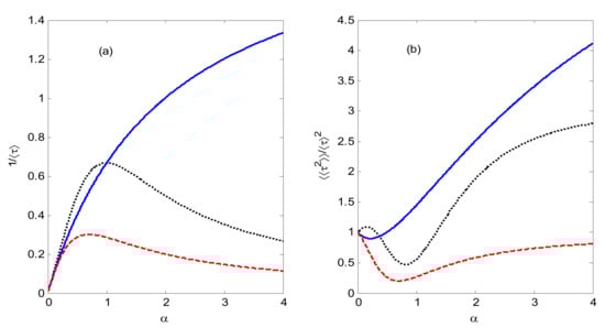
Figure 1.
(a) as a function of . (b) The randomness parameter, , as a function of . The blue solid line for constructive (), red dashed line for destructive (), and black dotted line for . The variable stands for the asymmetry of dot-state couplings to the left and right leads. .
The results show that the constructive interference () between the two channels leads to a super-Poisson noise, and the destructive interference () leads to a sub-Poisson noise, while the phase difference results in a sub-Poisson noise in a certain parameter range and a super-Poisson noise in another parameter range. This demonstrates that quantum interference can move the system back and forth between the sub-Poisson noise regime and the super-Poisson noise regime. Furthermore, the destructive interference () can lead to a small average current and a long average waiting time between two electron jumping events to the right lead.
Figure 2a exhibits the WTDs of the system for three different phase differences between two channels and the corresponding was shown as a function of time τ in Figure 2b. It shows that, for the constructive interference () case, the most probable waiting time and full width of WTDs are smaller than that of the other two cases, which leads to small average waiting time and large average current.
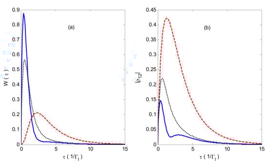
Figure 2.
(a) Waiting time distributions (WTDs) as a function of time . (b) as a function of time . The blue solid line is constructive (), red dashed line is destructive (), and black dotted line is . , .
Comparing Figure 2a,b, one can find that the smaller the decay rate of , the longer the average waiting time. The term represents the interference between the two channel states and is known as the coherence [35]. In order to enhance the interference between the two channel states, we decrease the value of , which can be understood from Equation (5).
Figure 3a exhibits the WTDs of the system for three different phase differences between the two channels; the corresponding values are shown as a function of time in Figure 3b. The parameter values of Figure 3 are the same as those of Figure 2, except . It is very interesting that the WTDs manifest oscillatory behavior with an increase in waiting time, which is an analog of the optical double-slit interference fringe. The oscillatory behavior of WTDs could not be found in the FCS results in the work of Wang and colleagues [27], which indicates that the WTDs can characterize the short-time physics and correlations in mesoscopic systems that are not accessible for FCS. These results also demonstrate that the phase differences between the two channels (the phase of ) are clearly reflected in the oscillation phase of the WTDs. Comparing the blue lines with the cyan lines, we observe that the oscillations of the WTDs decrease as the level spacing decreases. The effect of the level spacing is an analog of the slit spacing in optical double-slit interference.
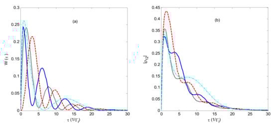
Figure 3.
(a) WTDs as a function of time . (b) as a function of time . The blue solid line is constructive (), red dashed line is destructive (), and black dotted line is . ; The cyan dot-dashed line is constructive (, , ); .
3.2. Non-Interacting Dots
Figure 4 shows and the randomness parameter, , as a function of the asymmetry of dot-state couplings to the left and right leads, respectively. This figure demonstrates that the phase difference between the two channel electrons jumping to the right lead has an obvious effect on the randomness parameter, while it has little effect on the average current; notably, the average currents are the same for the constructive interference () case and the destructive interference () case. Comparing Figure 4b with the corresponding Fano factor in the other work [27], we observe that the randomness parameter is different from the Fano factor of the system. Thus, the system is a nonrenewal system for non-interacting dots.
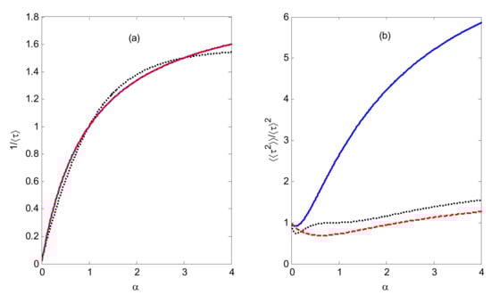
Figure 4.
(a) as a function of . (b) The randomness parameter, , as a function of . The blue solid line is constructive (), red dashed line is destructive (), and black dotted line is . Variable stands for the asymmetry of the dot-state couplings to the left and right leads..
Figure 5 exhibits the WTDs of the system for three different phase differences between the two channels as a function of time τ. Although the parameter values of Figure 5a are the same as those of Figure 3a, the oscillatory behaviors of the WTDs in Figure 3a disappear. This occurs because the presence of one excess electron inside the central dot system leads to no possibility for more than one electron at the same time to occupy the two channel states and destroys the coherent superposition of the two channel states. Figure 5b shows that, if we decrease the value of the electron tunneling rate Γl between the central QD and the left lead, the oscillatory behaviors of the WTDs appear because of the decrease in the probability that a double electron will occupy the central QD system. Figure 5 also shows that the probable density of the WTDs at time is nonzero, which suggests that it is now a multiple reset system because two electrons can be detected in the drain lead directly following one another for non-interacting dots. Comparing the blue line with the cyan line in Figure 5a, we observe that the WTD recovers some features of the oscillatory behavior as the level spacing increases.
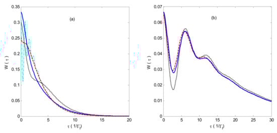
Figure 5.
WTDs as a function of time . (a) and (b) . The blue solid line is constructive (), red dashed line is destructive (), and black dotted line is , with ,; The cyan dot-dashed line is constructive (, , , ).
Figure 6 demonstrates the Pearson correlation coefficient p of the system for three different phase differences between the two channels as a function of the asymmetry of the dot-state couplings to the left and right leads with the same parameter values as those in Figure 5. Figure 6 shows that the electron waiting times are negatively correlated in the current case, in which a short waiting time is more likely to be followed by a long waiting time, and vice versa, because of the anti-bunching properties of fermion. Since we obtain the master equation under the Born–Markov approximation, the nonrenewal behavior of the system in the current case does not result from non-Markovian behavior.
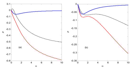
Figure 6.
The Pearson correlation coefficient p as a function of . (a) and (b) . The blue solid line is constructive (), red dashed line is destructive (), and black dotted line is . , .
Comparing Figure 6a,b, we also observe that the phase differences between the two channels obviously enhance the Pearson correlation coefficient. Furthermore, the Pearson correlation coefficient can be decreased by decreasing the value of the electron tunneling rate Γl, which can lead to a decrease in the probability of a double electron occupying the central QD system. This implies that the Pearson correlation coefficient is relative to the multiple reset characteristics. If the two channels of the QD system are doubly occupied, both electrons are likely to subsequently tunnel out, which leads to a short waiting time; then, the system will fill and empty again, which results in a long waiting time.
4. Conclusions
We are the first to employ the Born–Markov approximation to obtain a reduced particle-number resolved master equation for a two-channel QD system. Then, we investigated the WTD statistics of electron transport through a two-channel quantum system in a strong Coulomb blockade regime and for non-interacting dots. The influences of the phase differences between the two channels, the asymmetry of the dot-state couplings to the left and right electrodes, and Coulomb repulsion on the WTD statistics were investigated. The results show that these factors have obvious effects on the WTD statistics of the system.
First, the two-channel QD system in the strong Coulomb blockade regime is a single reset and renewal system, while the two-channel QD system in the non-interacting dots is a multiple reset and nonrenewal system.
Second, the phase differences between two channels, the asymmetry of the dot-state couplings to the left and right electrodes, and Coulomb repulsion have obvious effects on the WTD statistics of the system. In a certain parameter range, the system manifests the coherent oscillatory behavior of WTDs in a strong Coulomb blockade regime, and the phase differences between the two channels is clearly reflected in the oscillation phase of the WTDs. This oscillatory behavior is an analog of the optical double-slit interference fringe. The effect of the level spacing is an analog of slit spacing in optical double-slit interference.
Third, the electron waiting time of the system is negatively correlated when the two-channel QD system is for non-interacting dots. The different phase differences between the two channels can obviously enhance this negative correlation.
In brief, the short-time physics and correlations in mesoscopic systems can be characterized by WTDs, which are not accessible for FCS. The WTD statistics can be affected by the different phase differences between the two channels. The multiple reset system exhibits nonrenewal characteristics. These results deepen our understanding of the WTD statistical properties of electron transport through a mesoscopic QD system and help pave a new path toward constructing nanostructured QD electronic devices.
Author Contributions
W.L. prepared the manuscript, presented the concepts and theoretical derivation, and ran numerical calculations in this article. F.W. contributed to data analysis and manuscript preparation. R.L. carried out the study and collected important background information. All authors read and approved the final manuscript.
Funding
This work was funded by the National Natural Science Foundation of China (grant no. 61774062, no. 11674109); the Project of Department of Education of Guangdong Province; Science and Technology Planning Project of Guangdong Province, China (grant no. 2017A020219007); 2019 Natural Science Project of Guangzhou College of Technology and Business (grant no. KA201931); and the Research Fund Program of Guangdong Provincial Key Laboratory of Nanophotonic Functional Materials and Devices.
Conflicts of Interest
The authors declare no conflicts of interest.
References
- Deng, G.W.; Wei, D.; Li, S.X.; Johansson, J.R.; Kong, W.C.; Li, H.O.; Jiang, H.W. Coupling two distant double quantum dots with a microwave resonator. Nano Lett. 2015, 15, 6620–6625. [Google Scholar] [CrossRef]
- Delbecq, M.R.; Schmitt, V.; Parmentier, F.D.; Roch, N.; Viennot, J.J.; Fève, G.; Huard, B.; Mora, C.; Cottet, A.; Kontos, T. Coupling a quantum dot, fermionic leads, and a microwave cavity on a chip. Phys. Rev. Lett. 2011, 107, 256804. [Google Scholar] [CrossRef] [PubMed]
- Kulkarni, M.; Cotlet, O.; Türeci, H.E. Cavity-coupled double-quantum dot at finite bias: Analogy with lasers and beyond. Phys. Rev. B 2014, 90, 125402. [Google Scholar] [CrossRef]
- Agarwalla, B.K.; Kulkarni, M.; Mukamel, S.; Segal, D. Giant photon gain in large-scale quantum dot-circuit QED systems. Phys. Rev. B 2016, 94, 121305. [Google Scholar] [CrossRef]
- Levitov, L.S.; Lee, H.; Lesovik, G.B. Electron counting statistics and coherent states of electric current. J. Math. Phys. 1996, 37, 4845. [Google Scholar] [CrossRef]
- Blanter, Y.M.; Büttiker, M. Shot noise in mesoscopic conductors. Phys. Rep. 2000, 336, 1–166. [Google Scholar] [CrossRef]
- Bennett, S.D.; Clerk, A.A. Full counting statistics and conditional evolution in a nanoelectromechanical system. Phys. Rev. B 2008, 78, 165328. [Google Scholar] [CrossRef]
- Emary, C. Counting statistics of cotunneling electrons. Phys. Rev. B 2009, 80, 235306. [Google Scholar] [CrossRef]
- Tang, G.M.; Wang, J. Full-counting statistics of charge and spin transport in the transient regime: A nonequilibrium Green’s function approach. Phys. Rev. B 2014, 90, 195422. [Google Scholar] [CrossRef]
- Tang, G.M.; Yu, Z.Z.; Wang, J. Full-counting statistics of energy transport of molecular junctions in the polaronic regime. New J. Phys. 2017, 19, 083007. [Google Scholar] [CrossRef]
- Ashida, Y.; Ueda, M. Full-counting many-particle dynamics: Nonlocal and chiral propagation of correlations. Phys. Rev. Lett. 2018, 120, 185301. [Google Scholar] [CrossRef] [PubMed]
- Fujisawa, T.; Hayashi, T.; Tomita, R.; Hirayama, Y. Bidirectional Counting of Single Electrons. Science 2006, 312, 1634–1636. [Google Scholar] [CrossRef] [PubMed]
- Albert, M.; Flindt, C.; Büttiker, M. Distributions of waiting times of dynamic single-electron emitters. Phys. Rev. Lett. 2011, 107, 086805. [Google Scholar] [CrossRef] [PubMed]
- Albert, M.; Haack, G.; Flindt, C.; Büttiker, M. Electron waiting times in mesoscopic conductors. Phys. Rev. Lett. 2012, 108, 186806. [Google Scholar] [CrossRef] [PubMed]
- Dasenbrook, D.; Hofer, P.P.; Flindt, C. Electron waiting times in coherent conductors are correlated. Phys. Rev. B 2015, 91, 195420. [Google Scholar] [CrossRef]
- Ptaszyński, K. Waiting time distribution revealing the internal spin dynamics in a double quantum dot. Phys. Rev. B 2017, 96, 035409. [Google Scholar] [CrossRef]
- Thomas, K.H.; Flindt, C. Electron waiting times in non- Markovian quantum transport. Phys. Rev. B 2013, 87, 121405. [Google Scholar] [CrossRef]
- Sothmann, B. Electronic waiting-time distribution of a quantum-dot spin valve. Phys. Rev. B 2014, 90, 155315. [Google Scholar] [CrossRef]
- Ptaszyński, K. Nonrenewal statistics in transport through quantum dots. Phys. Rev. B 2017, 95, 045306. [Google Scholar] [CrossRef]
- Hofer, P.P.; Dasenbrook, D.; Flindt, C. Electron waiting times for the mesoscopic capacitor. Physica E 2016, 82, 3–11. [Google Scholar] [CrossRef]
- Rajabi, L.; Pöltl, C.; Governale, M. Waiting Time Distributions for the Transport through a Quantum-Dot Tunnel Coupled to One Normal and One Superconducting Lead. Phys. Rev. Lett. 2013, 111, 067002. [Google Scholar] [CrossRef] [PubMed]
- Chevallier, D.; Albert, M.; Devillard, P. Probing Majorana and Andreev bound states with waiting times. Eur. Lett. 2016, 116, 27005. [Google Scholar] [CrossRef][Green Version]
- Brandes, T. Waiting times and noise in single particle transport. Ann. Der Phys. 2008, 17, 477–496. [Google Scholar] [CrossRef]
- Kosov, D.S. Waiting time distribution for electron transport in a molecular junction with electron-vibration interaction. J. Chem. Phys. 2017, 146, 074102. [Google Scholar] [CrossRef] [PubMed]
- Rudge, S.L.; Kosov, D.S. Nonrenewal statistics in quantum transport from the perspective of first-passage and waiting time distributions. Phys. Rev. B 2019, 99, 115426. [Google Scholar] [CrossRef]
- Rudge, S.L.; Kosov, D.S. Distribution of waiting times between electron cotunneling events. Phys. Rev. B 2018, 98, 245402. [Google Scholar] [CrossRef]
- Wang, S.K.; Jiao, H.; Li, F.; Li, X.Q.; Yan, Y. Full counting statistics of transport through two-channel Coulomb blockade systems. Phys. Rev. B 2007, 76, 125416. [Google Scholar] [CrossRef]
- Timm, C. Tunneling through molecules and quantum dots: Master-equation approaches. Phys. Rev. B 2008, 77, 195416. [Google Scholar] [CrossRef]
- Schuster, R.; Buks, E.; Heiblum, M.; Mahalu, D.; Umansky, V.; Shtrikman, H. Phase measurement in a quantum dot via a double-slit interference experiment. Nature 1997, 385, 417. [Google Scholar] [CrossRef]
- Entin-Wohlman, O.; Aharony, A.; Imry, Y.; Levinson, Y.; Schiller, A. Broken unitarity and phase measurements in Aharonov-Bohm interferometers. Phys. Rev. Lett. 2002, 88, 166801. [Google Scholar] [CrossRef]
- Avinun-Kalish, M.; Heiblum, M.; Zarchin, O.; Mahalu, D.; Umansky, V. Crossover from ‘mesoscopic’to ‘universal’phase for electron transmission in quantum dots. Nature 2005, 436, 529. [Google Scholar] [CrossRef] [PubMed]
- Santamore, D.H.; Neill, L.; Franco, N. Vibrationally mediated transport in molecular transistors. Phys. Rev. B 2013, 87, 075422. [Google Scholar] [CrossRef]
- Walter, S.; Trauzettel, B.; Schmidt, T.L. Transport properties of double quantum dots with electron-phonon coupling. Phys. Rev. B 2013, 88, 195425. [Google Scholar] [CrossRef]
- Brange, F.; Menczel, P.; Flindt, C. Photon counting statistics of a microwave cavity. Phys. Rev. B 2019, 99, 085418. [Google Scholar] [CrossRef]
- Woldeyohannes, M.; John, S. Coherent control of spontaneous emission near a photonic band edge. J. Opt. B 2003, 5, R43. [Google Scholar] [CrossRef]


© 2020 by the authors. Licensee MDPI, Basel, Switzerland. This article is an open access article distributed under the terms and conditions of the Creative Commons Attribution (CC BY) license (http://creativecommons.org/licenses/by/4.0/).