Condition Monitoring System and Faults Detection for Impedance Bonds from Railway Infrastructure

 ,
, 
 , ,
, ,  and
and 
Abstract
1. Introduction
- -
- to ensure the return circuit of the electric traction current;
- -
- to separate the signaling current of the track circuit from the traction current;
- -
- to control and to signal the trains circulation;
- -
- to ensure the protection of the installations from the contact line vicinity.
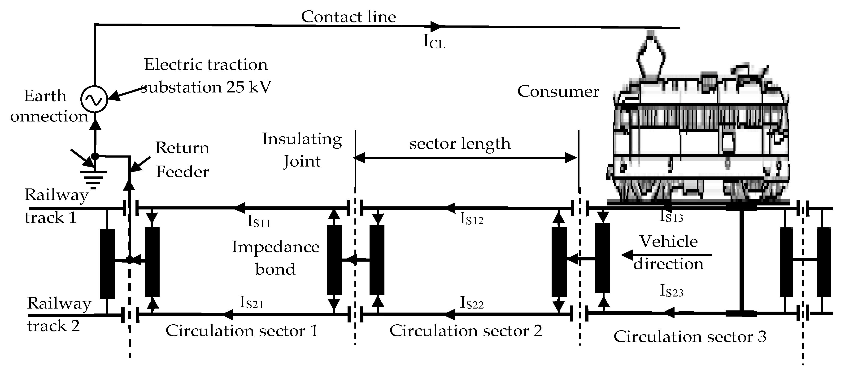
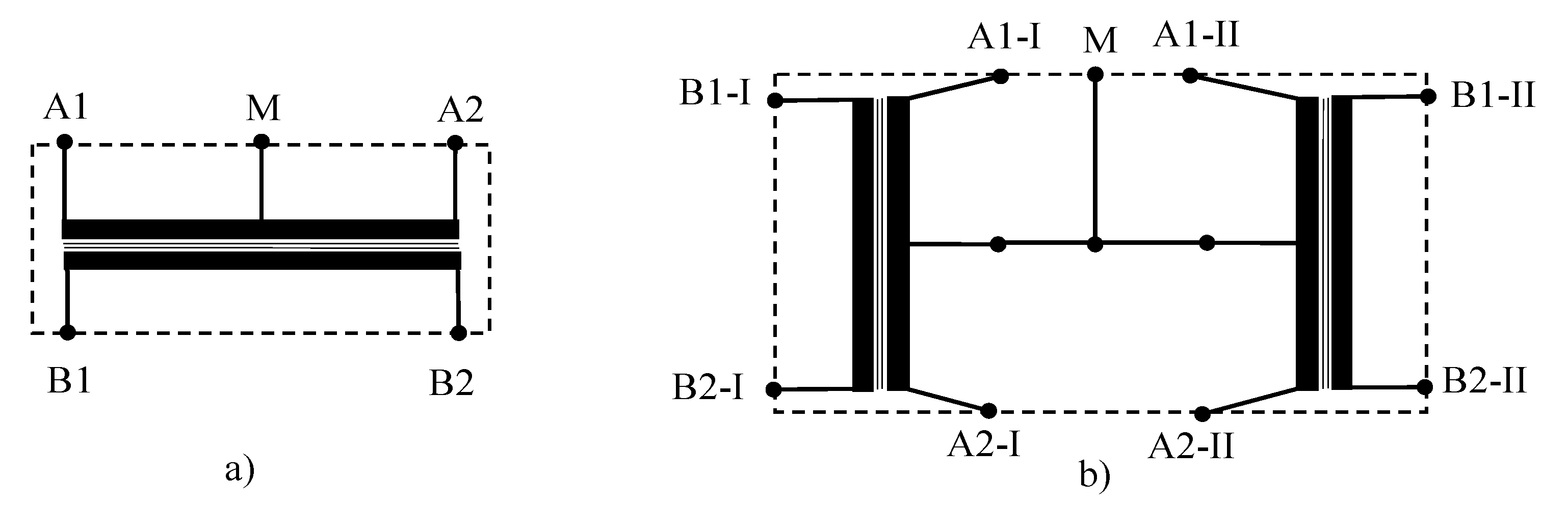
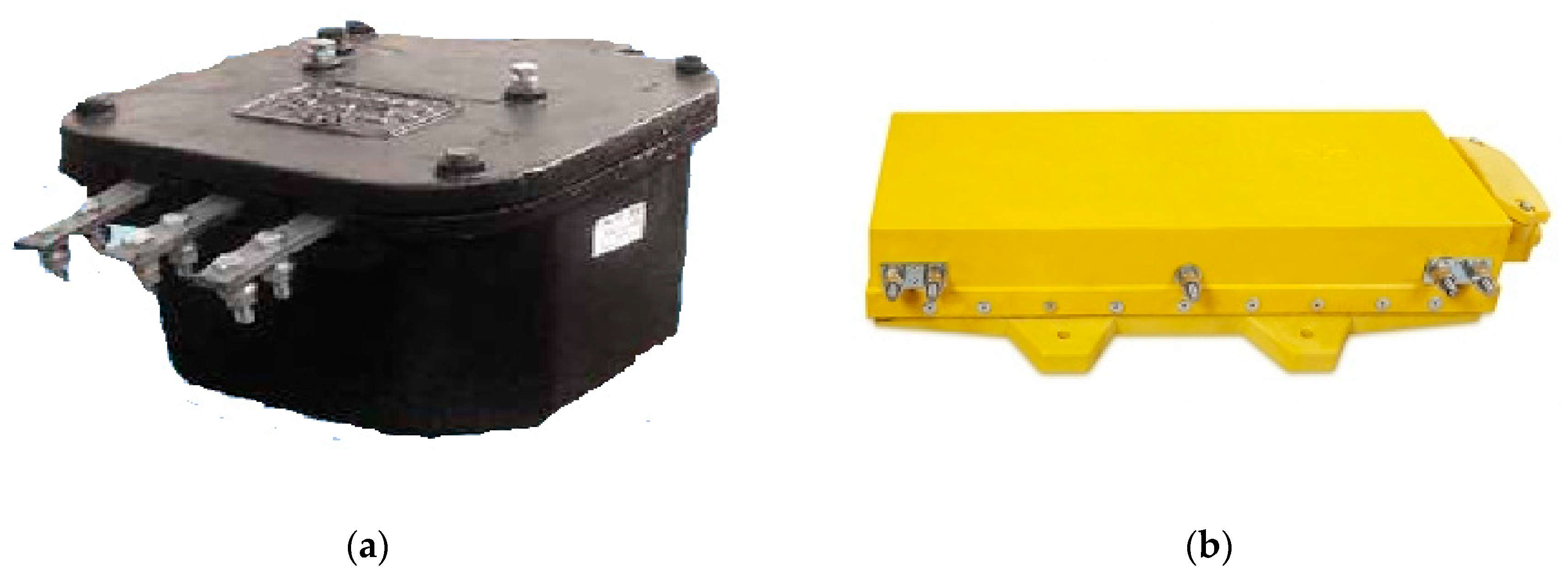
2. Aspects about the Impedance Bond of the Return Circuit from the Power Supply System of Railway Infrastructure
- overhead line or underground line to supply the electric traction substations;
- electric traction substations that ensure the reduction of the AC voltage level to the value required to power supply the contact line, 25 kV;
- electrical installations and equipment for supplying the contact line (power supply feeder, return feeder);
- the contact line, built along the railway, is an overhead electrical network that power supplies the consumers (locomotives and electric frames) from the electric traction;
- section post, subsection post for transverse, and longitudinal sectioning of the contact line;
- the railway tracks, which have a dual role, namely: of the track running and of the return conductor for the current to the electric traction substation;
- consumers (locomotive and electric frame, internal consumers);
- devices for monitoring, diagnosis, remote control, and remote signaling of the power supply system.
3. Condition Monitoring of the Impedance Bonds
3.1. Aspects about Monitoring and Possible Faults of the Impedance Bonds
- oxidized electrical contacts;
- insufficient tightening of the connection terminals;
- interruption (sometimes lack) of the connecting cables between the impedance bond terminals and the railway track;
- interruption of the railway track;
- short-circuit in the winding of impedance bond;
- interruption of the track circuit.
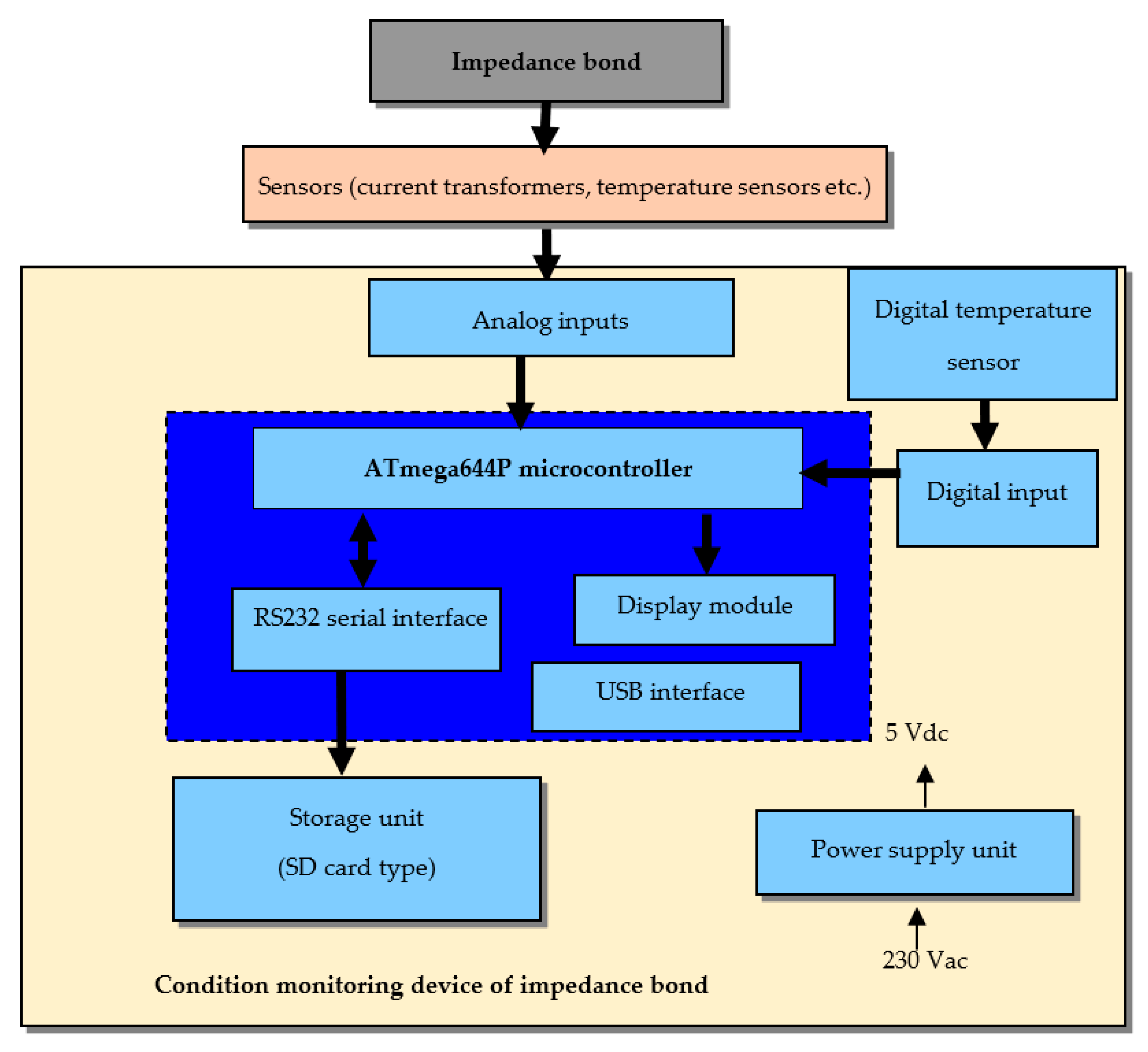
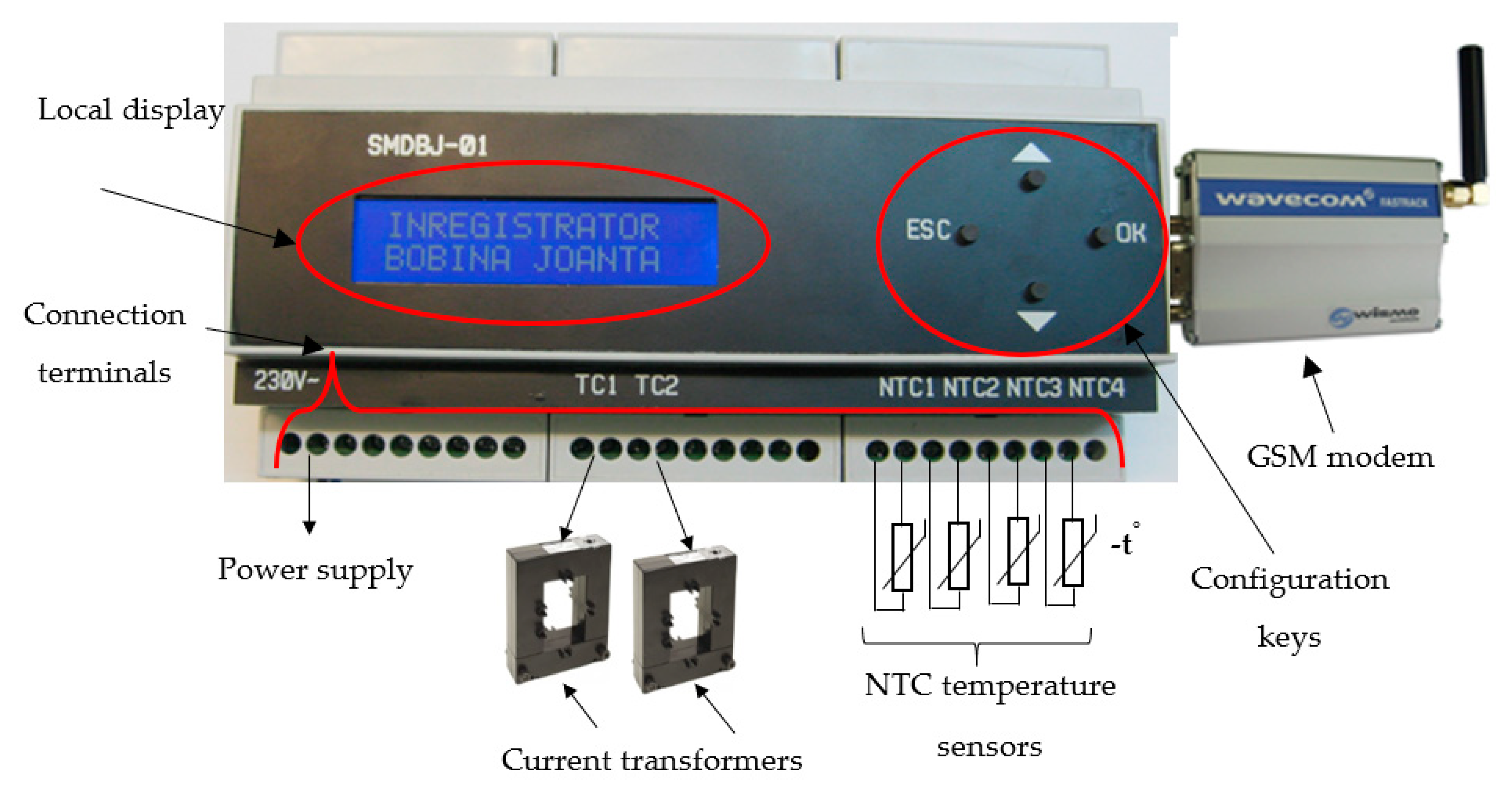
3.2. Condition Monitoring Device and Sensors Used for Monitoring the Impedance Bonds
- ATmega644P microcontroller;
- two current transducers based on Hall effect of LEM LTS 6-NP type;
- two current transformers;
- four Negative Temperature Coefficient (NTC) temperature sensors;
- digital temperature sensor of DS18B20 type;
- power supply module of Tracopower TMLM 04105 type;
- communication interfaces with TTL/RS232 converter and TTL/USB converter;
- SD-card module of ROGUE uMMC type for local data storage;
- 2 × 16-character liquid crystal display, for monitoring device configuration and data displaying;
- GSM modem.
- direct supply from the operative voltage (230 V AC);
- displaying on LCD the temperatures acquired from each sensor of the impedance bond, as well as the traction current;
- recording all the parameters on an SD-card;
- sending alarms via a communication interface (GSM) to an operator.
- the traction currents on the two railway tracks;
- the current imbalance between the two railway tracks;
- interrupting a connection cable to one of the railway tracks;
- the temperature on each terminal and the connection ropes;
- the temperature from the impedance bond housing.
3.2.1. Current Transformers
3.2.2. Current Transducers with Hall Effect
3.2.3. Temperature Sensors
3.2.4. Digital Temperature Sensors
- exceeding a minimum/maximum temperature limit for each monitored temperature point;
- exceeding the maximum current allowed by each half impedance bond winding;
- exceeding a maximum allowable imbalance between the currents on each rail;
- detecting the interruption of a connection cable.
4. Results
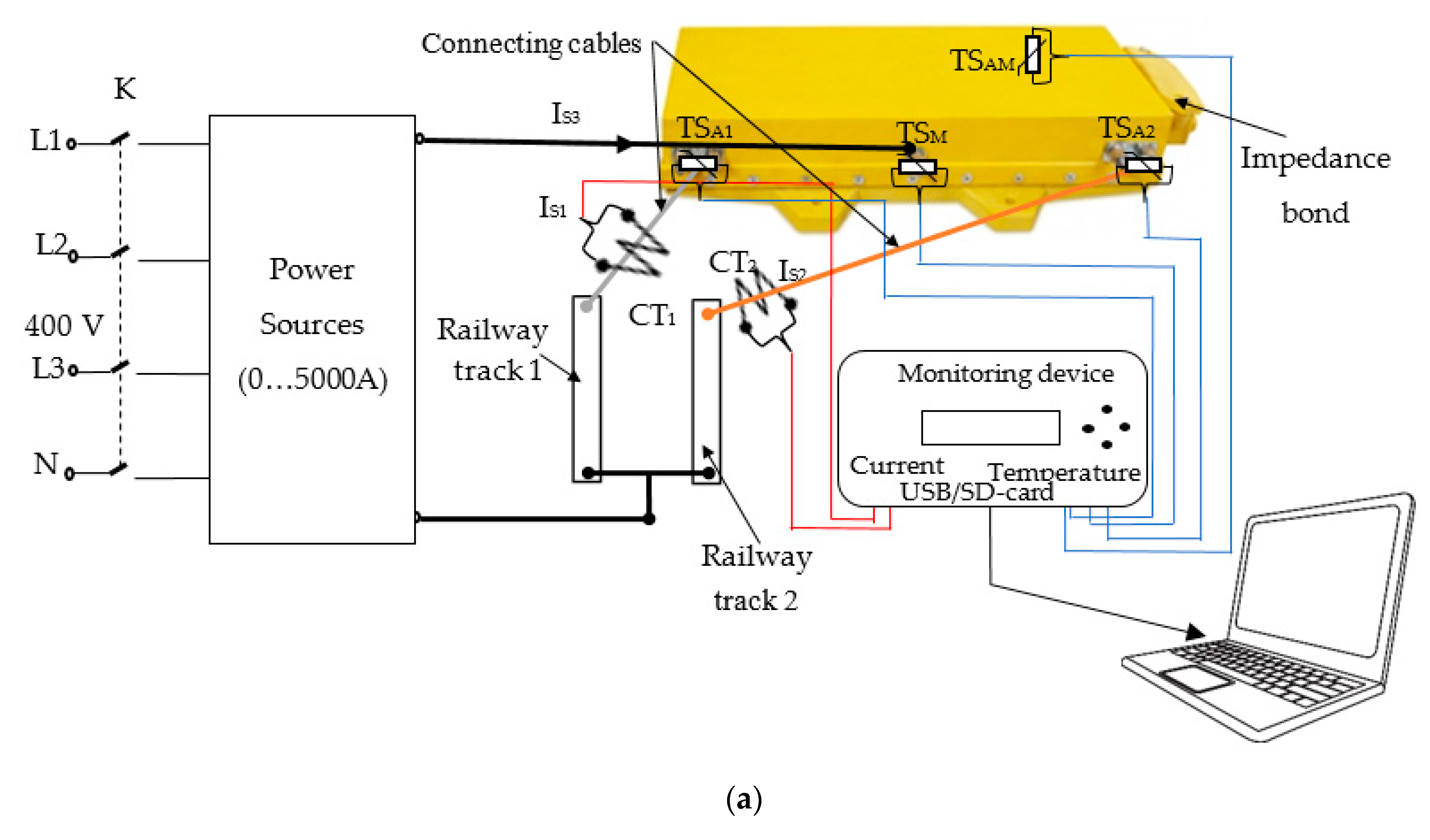
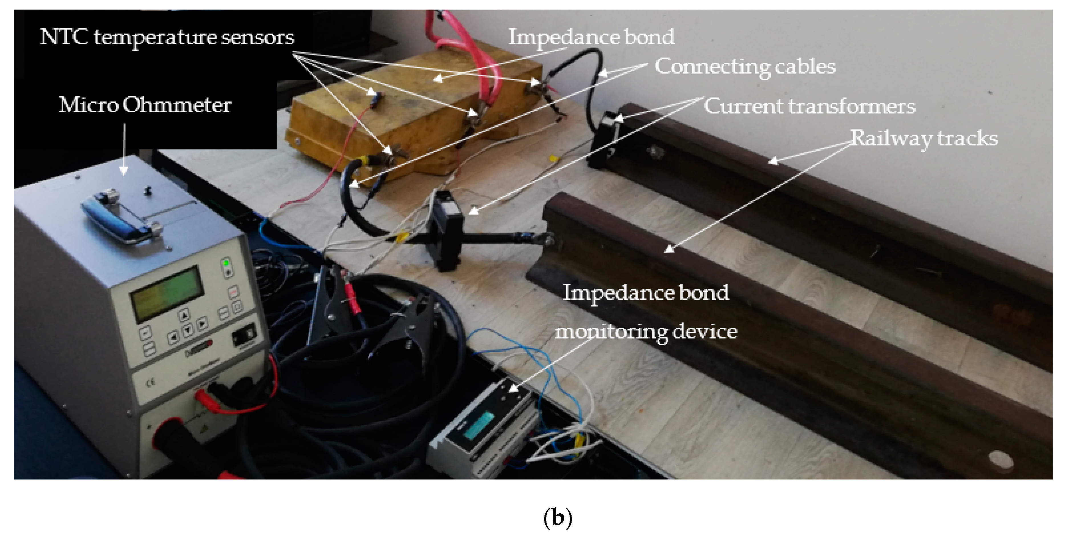
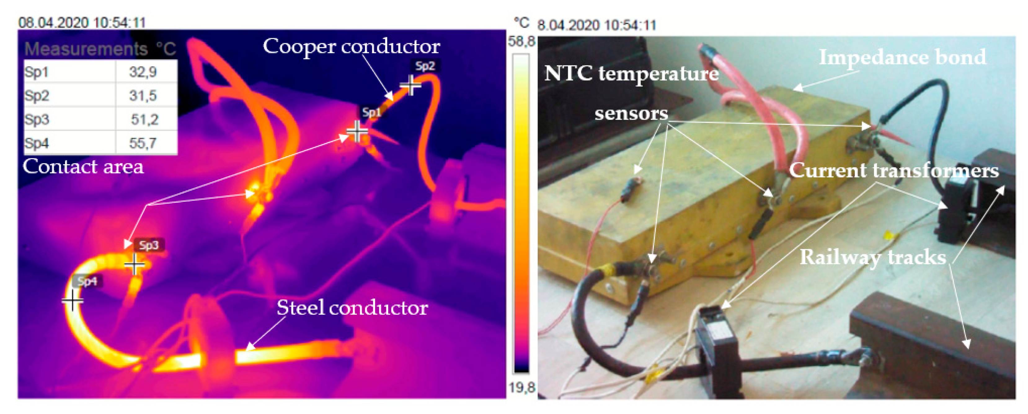
4.1. Experimental Installation for Testing of the Impedance Bond with Condition Monitoring Device and Faults Detection
- a healthy condition—connecting the railway tracks with the impedance bond through a copper cable with a section of 50 mm2 with PVC insulation;
- a healthy condition—connecting the railway tracks with the impedance bond through two steel cable with a section of 78 mm2 with PVC insulation;
- a faulty condition—connecting the railway tracks with the impedance bond through one steel cable with a section of 78 mm2 with PVC insulation. This fault may occur when a steel cable between the impedance bond terminals and the railway track are interrupted;
- a faulty condition—insufficient tightening of the connection terminals. The appearance of this fault in the return circuit is explained by loosening the tightening of screw nuts, oxidation, rust, etc.
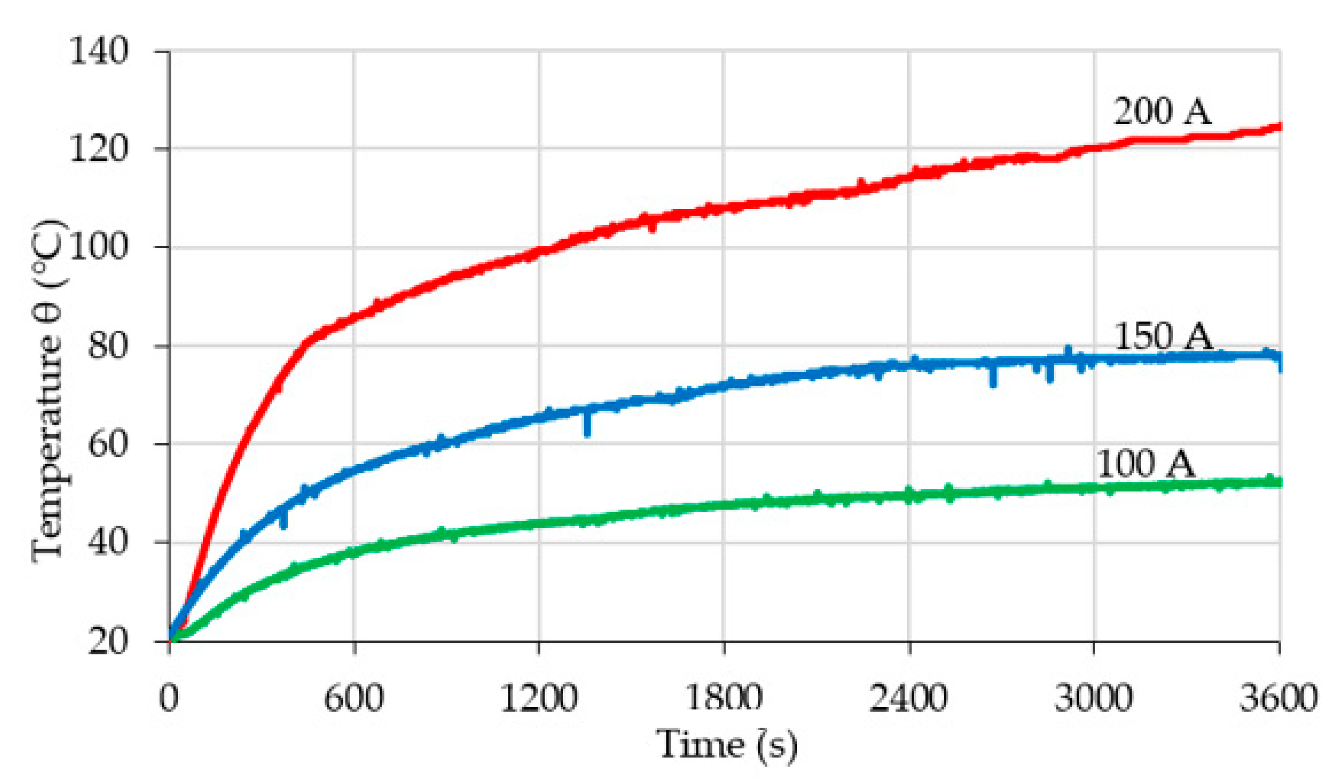
4.2. First Case—Healthy Condition When the Connection of the Railway Tracks with the Impedance Bond Is Made through a Copper Cable with a Section of 50 mm2 with PVC Insulation
4.3. Second Case—Healthy Condition When the Connection of the Railway Tracks with the Impedance Bond Is Made through Two Steel Cables with a Section of 78 mm2 with PVC Insulation
4.4. Third Case—Faulty Condition When Connecting the Railway Tracks with the Impedance Bond Is Made through One Steel Cable with a Section of 78 mm2 with PVC Insulation
- ambient temperature: 20 °C;
- the emissivity index: this parameter has been set to the value of 0.9;
- reflected temperature: set equal to ambient temperature, 20 °C;
- relative humidity of the air: the value measured in the laboratory at the time of the experiment was 55%;
- the distance from the camera lens to the investigated connection was 1.5 m;
- the temperature range was selected from −30 to 160 °C.
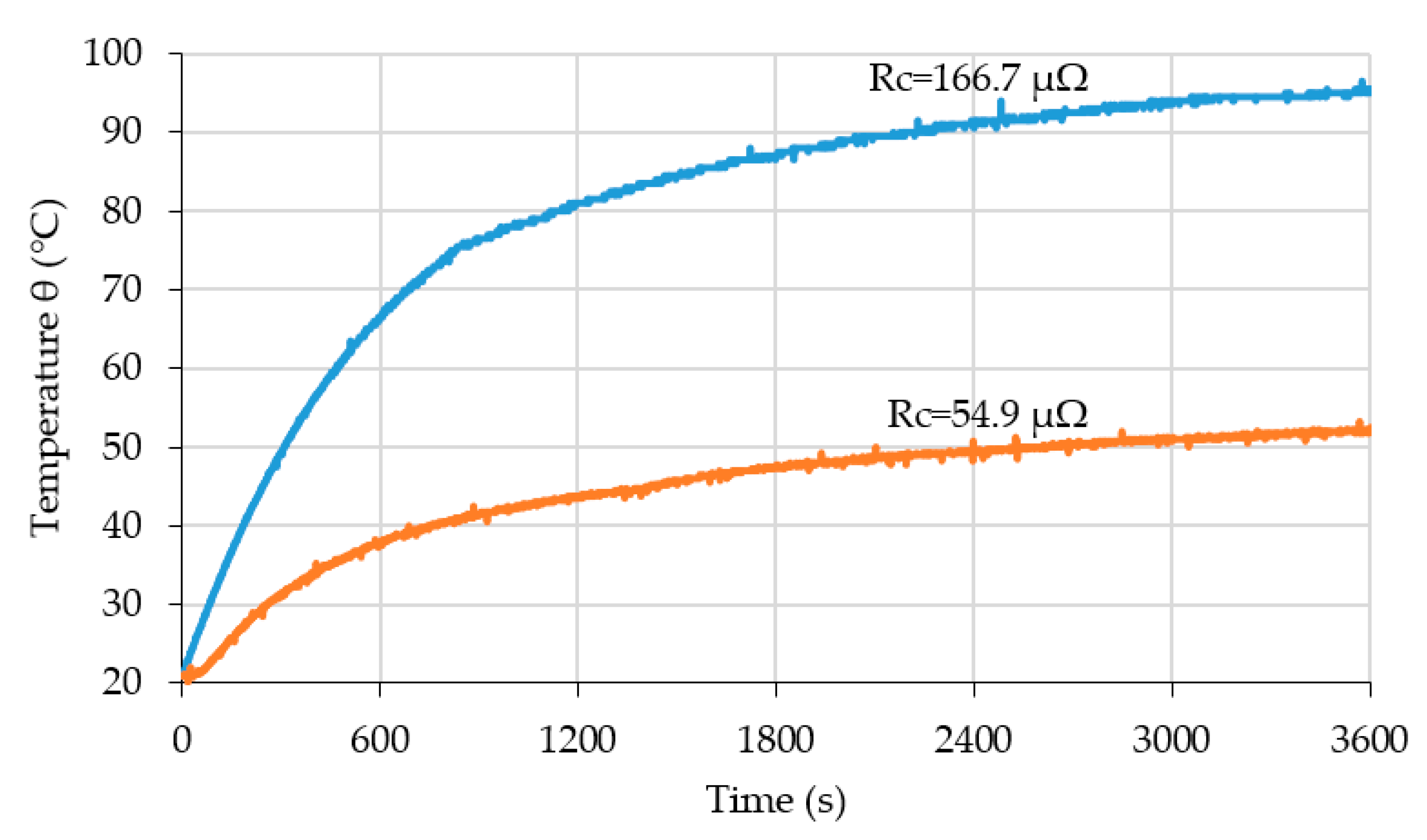
4.5. Fourth Case—Faulty Condition with Insufficient Tightening (High Contact Resistance) of the Connection Terminals
5. Conclusions
- knowing the currents through the two primary coils of the impedance bond, the temperatures on the contact terminals, on the metallic or non-metallic housing of the coil, and the ambient temperatures;
- impedance bond diagnosis (a higher temperature in the contact areas, a higher of the current imbalance through the two running rails, the interruption of the connecting conductors between the impedance bond terminals and railway track, etc.);
- real-time knowledge of the technical condition of the impedance bond by analyzing the acquired data and comparing it with previous records;
- the device has high flexibility, both at the hardware structure (the possibilities of extending of inputs number, respectively, possibly extending the storage capacity), and also to the software (upgrading the firmware at the device location).
6. Patents
Author Contributions
Funding
Acknowledgments
Conflicts of Interest
References
- Tsunashima, H. Condition monitoring of railway tracks from car-body vibration using a machine learning technique. Appl. Sci. 2019, 9, 2734. [Google Scholar] [CrossRef]
- Garramiola, F.; Poza, J.; Olmo, J.; Madina, P.; Almandoz, G. Integral sensor fault detection and isolation for railway traction drive. Sensors 2018, 18, 1543. [Google Scholar] [CrossRef] [PubMed]
- Berlin, E.; Laerhoven Van, K. Sensor networks for railway monitoring: Detecting trains from their distributed vibration footprints. In Proceedings of the 2013 IEEE International Conference on Distributed Computing in Sensor Systems, Cambridge, MA, USA, 20–23 May 2013. [Google Scholar]
- Chen, J.; Roberts, C.; Weston, P. Fault detection and diagnosis for railway track circuits using neuro-fuzzy systems. Control Eng. Pract. 2008, 16, 585–596. [Google Scholar] [CrossRef]
- Zhao, L.H.; Wu, J.P.; Ran, Y.K. Fault diagnosis for track circuit using AOK-TFRs and AGA. Control Eng. Pract. 2012, 20, 1270–1280. [Google Scholar]
- Hodge, V.; O’Keefe, S.; Weeks, M.; Moulds, A. Wireless sensor networks for condition monitoring in the railway industry: A survey. IEEE Trans. Intell. Transp. Syst. 2015, 16, 1088–1106. [Google Scholar] [CrossRef]
- Ngamkhanong, C.; Kaewunruen, S.; Afonso Costa, B. State-of-the-art review of railway track resilience monitoring. Infrastructures 2018, 3, 3. [Google Scholar] [CrossRef]
- Bernal, E.; Spiryagin, M.; Cole, C. Onboard condition monitoring sensors, systems and techniques for freight railway vehicles: A review. IEEE Sens. J. 2019, 19, 4–24. [Google Scholar] [CrossRef]
- Gardea, C.; Dumitru, D.; Ciobotar, A.; Niculescu, O. Impedance Bond. Romania Patent RO 123523 B1, 29 May 2013. [Google Scholar]
- Sando, D.; Lakes, L. Double Impedance Bond. U.S. Patent US 8,333,350 B2, 18 December 2012. [Google Scholar]
- Munteanu, A.; Adam, M.; Andrusca, M.; Dragomir, A.; Boghiu, E. Aspects regarding the monitoring of electrical equipment from electric traction. In Proceedings of the 10th EPE 2018, Iaşi, Romania, 18–19 October 2018. [Google Scholar]
- Adam, M.; Munteanu, A.; Pancu, C.M.; Andrusca, M. Method and Apparatus for Monitoring and Diagnosis of Impedance Bond. Romania Patent Request nr. a 00233, 29 September 2017. [Google Scholar]
- Bruin, T.; Verbert, K.; Robert Babuska, R. Railway track circuit fault diagnosis using recurrent neural networks. IEEE Trans. Neural Netw. Learn. Syst. 2016, 28, 523–533. [Google Scholar] [CrossRef]
- Yuan, L.; Yang, Y.; Hernández, A.; Shi, L. Feature extraction for track section status classification based on UGW signals. Sensors 2018, 18, 1225. [Google Scholar] [CrossRef]
- Polivka, A.L.; West, P.; Malone, J.; Smith, B.E.; Renfrow, S.M. System and Method for Detecting Broken Rail and Occupied Track from a Railway Vehicle. U.S. Patent US 9,162,691 B2, 20 October 2015. [Google Scholar]
- Turabimana, P.; Nkundineza, C. Development of an onboard measurement system for railway vehicle wheel flange wear. Sensors 2020, 20, 303. [Google Scholar] [CrossRef]
- Tsunashima, H.; Kojima, T.; Marumo, Y.; Matsumoto, H.; Mizuma, T. Condition monitoring of railway track using in-service vehicle. In Proceedings of the 4th IET International Conference of Railway Condition Monitoring, Derby, UK, 18–20 June 2008. [Google Scholar]
- Tsunashima, H.; Naganuma, Y.; Matsumoto, A.; Mizuma, T.; Mori, H. Japanese Railway Condition Monitoring of Tracks using in-Service Vehicle. In Proceedings of the 5th IET Conference on Railway Condition Monitoring and Non-Destructive Testing (RCM 2011), Derby, UK, 29–30 November 2011. [Google Scholar]
- Tsunashima, H.; Mori, H.; Yanagisawa, K.; Ogino, M.; Asano, A. Condition monitoring of railway tracks using compact size on-board monitoring device. In Proceedings of the 6th IET Conference on Railway Condition Monitoring (RCM), Birmingham, UK, 17–18 September 2014. [Google Scholar]
- Chen, J.; Díaz, M.; Rubio, B.; Troya, J.M. RAISE: Railway Infrastructure health monitoring using wireless sensor networks. Sens. Syst. Softw. 2013, 122, 143–157. [Google Scholar]
- Bennett, P.J.; Soga, K.; Wassell, I.; Fidler, P.; Abe, K.; Kobayashi, Y.; Vanicek, M. Wireless sensor networks for underground railway Applications: Case studies in Prague and London. Smart Struct. Syst. 2010, 6, 619–639. [Google Scholar] [CrossRef]
- Flammini, F.; Gaglione, A.; Ottello, F.; Pappalardo, A.; Pragliola, C.; Tedesco, A. Towards wireless sensor networks for railway infrastructure monitoring. In Proceedings of the Electrical Systems for Aircraft, Railway and Ship Propulsion, Bologna, Italy, 19–21 October 2010; pp. 1–6. [Google Scholar]
- Bin, S.; Sun, G. Optimal energy resources allocation method of wireless sensor networks for intelligent railway systems. Sensors 2020, 20, 482. [Google Scholar] [CrossRef] [PubMed]
- Gao, M.; Wang, P.; Wang, Y.; Yao, L. Self-Powered ZigBee Wireless sensor nodes for railway condition monitoring. IEEE Trans. Intell. Transp. Syst. 2018, 19, 900–909. [Google Scholar] [CrossRef]
- Gao, M.; Li, Y.; Lu, J.; Wang, Y.; Wang, P.; Wang, L. Condition monitoring of urban rail transit by local energy harvesting. Intern. J. Distrib. Sens. Netw. 2018, 14, 1550147718814469. [Google Scholar] [CrossRef]
- Buggy, S.; James, S.W.; Carroll, R.; Jaiswal, J.; Staines, S.; Tatam, R.P. Intelligent infrastructure for rail and tramways using Optical fibre sensors. In Proceedings of the IET Railway Young Professionals, Best Paper Competition, London, UK, 16–18 November 2011. [Google Scholar]
- Garramiola, F.; Poza, J.; Olmo, J.; Madina, P.; Almandoz, G. DC-link voltage and catenary current sensors fault reconstruction for railway traction drives. Sensors 2018, 18, 1998. [Google Scholar] [CrossRef]
- Mariscotti, A.; Pozzobon, P. Determination of the electrical parameters of railway traction lines: Calculation, measurement and reference data. IEEE Trans. Power Deliv. 2004, 19, 1538–1546. [Google Scholar] [CrossRef]
- Mariscotti, A. Direct measurement of power quality over railway networks with results of a 16.7 Hz network. IEEE Trans. Instrum. Meas. 2011, 60, 1604–1612. [Google Scholar] [CrossRef]
- Dolara, A.; Gualdoni, M.; Leva, S. Impact of high-voltage primary supply lines in the 2 × 25 kV, 50 Hz railway system on the equivalent impedance at pantograph terminals. IEEE Trans. Power Deliv. 2012, 27, 164–175. [Google Scholar] [CrossRef]
- Chiriac, G.; Nituca, C.; Cardasim, M. Failures analysis in the 25 kV/50 Hz railway substations. In Proceedings of the 2017 International Conference on Electromechanical and Power Systems (SIELMEN), Iasi, Romania, 11–13 October 2017. [Google Scholar]
- Onea, R. Construction, Operation and Maintenance of Fixed Railway Traction Installations; Publisher ASAB: Bucharest, Romania, 2004. [Google Scholar]
- Mariscotti, A. Distribution of the traction return current in AC and DC electric railways systems. IEEE Trans. Instr. Meas. 2003, 18, 1422–1432. [Google Scholar] [CrossRef]
- Munteanu, A.; Adam, M.; Andrusca, M.; Dragomir, A.; Boghiu, E. Possibility to monitoring and diagnosis the joint coils from electric traction. In Proceedings of the 10th EPE 2018, Iaşi, România, 18–19 October 2018. [Google Scholar]
- Filograno, M.L.; Guillén, P.C.; Rodríguez-Barrios, A.; Martín-López, S.; Rodríguez-Plaza, M.; Andrés-Alguacil, Á.; González-Herráez, M. Real-time monitoring of railway traffic using Fiber Bragg grating sensors. IEEE Sens. J. 2012, 12, 85–92. [Google Scholar] [CrossRef]


| Impedance bond monitoring | Parameters/Characteristic | Techniques and Devices | Monitoring Possibility |
| Contact resistance | Measurement of the resistance by the volt-ampere method. (Static contact resistance) | online/offline | |
| Contact temperature | Infrared techniques. Temperature measurement at one point with the thermocouple, thermistor, optical sensor, infrared sensor, etc. | online | |
| Current through the impedance bond | Measuring the current with current transformers with ferromagnetic core, with air core (Rogowski coils), hall effect transducers, optical current sensor. | online | |
| Partial discharges | Ultrasonic and acoustic vibrations. Ultrasonic sensors, online acoustic emission technique | online | |
| Oil level | Electronic, optical or mechanical level indicator online | online | |
| Oil quality | Determination of moisture content, acidity, dissolved gas analysis, power factor measurement | offline | |
| Coil impedance | Measurement by direct methods with special devices, respectively indirect methods (volt-ampere method) | online/offline |
| Technical Specifications | |
|---|---|
| Number of current inputs | 2 |
| Current measurement range | 0 … 300 A |
| Current accuracy | ±3% |
| Current measurement resolution | 0.1 A |
| Current transducer on PCB | LEM 6 A type |
| Number of temperature inputs | 5 |
| Temperature measurement range | −40 °C … 250 °C |
| Temperature measurement resolution | 0.1 °C |
| Temperature sensor | NTC thermistor type |
| Temperature accuracy | ±2% |
| Programming mode | ISP connector |
| Communication interface | RS 232, USB, GSM |
| Data recording | PC, SD-card |
| Card type | SD/miniSD/microSD |
| SD-card memory | 8 MB … 32 GB |
| Display | LCD 16 × 2 characters, lighting |
| Operating temperature | −40 °C … +85 °C |
| Power supply | 90 … 264 Vca |
| Exterior dimensions | 90 × 155 × 60 mm |
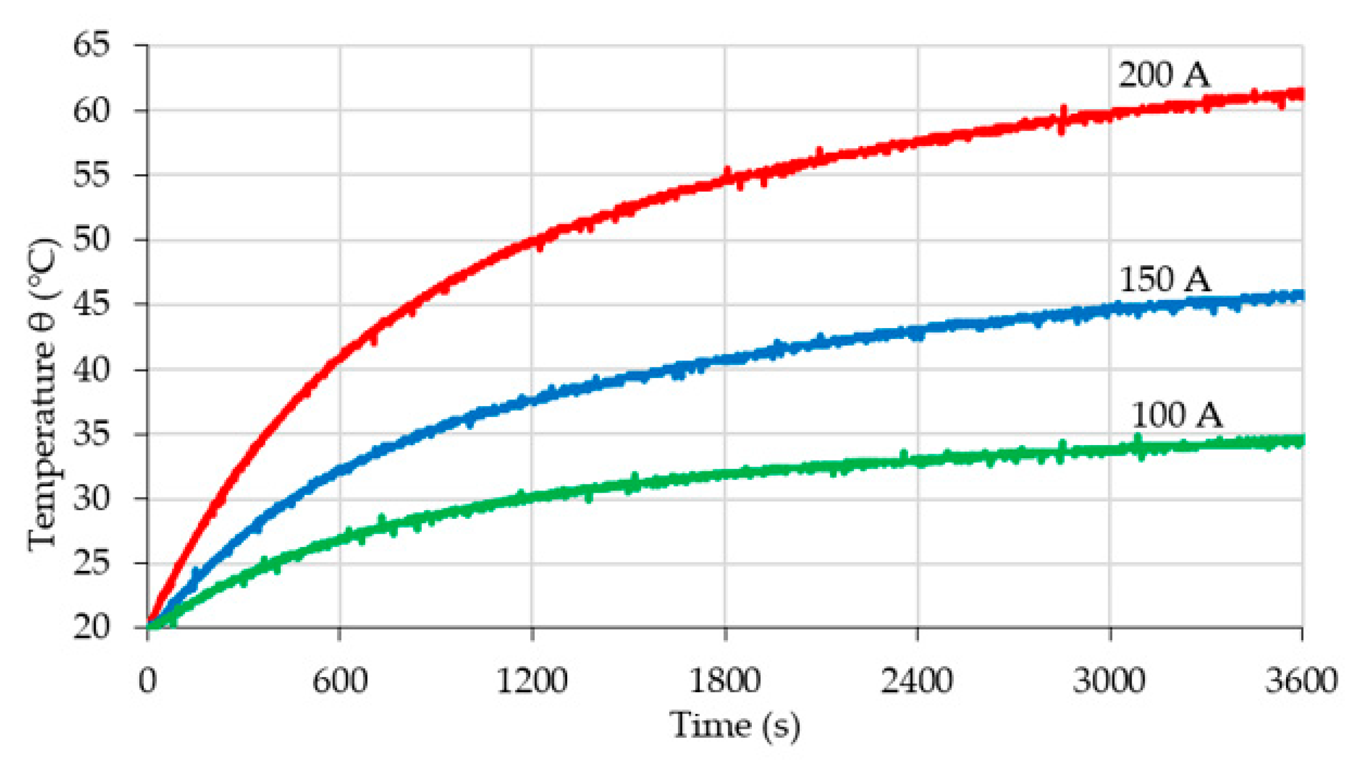
| Case | Connecting Mode between Impedance Bond Terminal and Railway Track | Rc (μΩ) | ||
|---|---|---|---|---|
| 100 A | 150 A | 200 A | ||
| 1 | With a copper connecting cable | 59.8 | 58.2 | 55.3 |
| 2 | With two steel connecting cables | 27.1 | 27.4 | 27.3 |
| 3 | With a steel connecting cable | 54.9 | 53.8 | 46.3 |
© 2020 by the authors. Licensee MDPI, Basel, Switzerland. This article is an open access article distributed under the terms and conditions of the Creative Commons Attribution (CC BY) license (http://creativecommons.org/licenses/by/4.0/).
Share and Cite
Andrusca, M.; Adam, M.; Dragomir, A.; Lunca, E.; Seeram, R.; Postolache, O. Condition Monitoring System and Faults Detection for Impedance Bonds from Railway Infrastructure. Appl. Sci. 2020, 10, 6167. https://doi.org/10.3390/app10186167
Andrusca M, Adam M, Dragomir A, Lunca E, Seeram R, Postolache O. Condition Monitoring System and Faults Detection for Impedance Bonds from Railway Infrastructure. Applied Sciences. 2020; 10(18):6167. https://doi.org/10.3390/app10186167
Chicago/Turabian StyleAndrusca, Mihai, Maricel Adam, Alin Dragomir, Eduard Lunca, Ramakrishna Seeram, and Octavian Postolache. 2020. "Condition Monitoring System and Faults Detection for Impedance Bonds from Railway Infrastructure" Applied Sciences 10, no. 18: 6167. https://doi.org/10.3390/app10186167
APA StyleAndrusca, M., Adam, M., Dragomir, A., Lunca, E., Seeram, R., & Postolache, O. (2020). Condition Monitoring System and Faults Detection for Impedance Bonds from Railway Infrastructure. Applied Sciences, 10(18), 6167. https://doi.org/10.3390/app10186167