Abstract
Research on Consumption-Based Carbon Footprints has recognised that lifestyles change significantly along the urban–rural continuum, with urban typically manifesting as an increase in the footprint of consumption while rural areas have a higher footprint for vehicle usage. However, there is limited research on the extent to which land-use patterns defined by urban plans influence these outcomes. To fill this lack, we controlled for household income and housing type and measured Spearman and Pearson partial correlations between the coverage of different zoning land-use types in the neighbourhoods and the footprints of different subdomains: Goods and services, Leisure travel, Vehicle, and Total footprint. These domains are central to both modern lifestyles and urban planning with related objectives. We found out that high Goods and Services and Leisure travel footprints do align with the urban land-use types, while Vehicle footprints show inverted results. However, the mirrored impact for higher Vehicle and Total footprint is not recognised in exurban areas, while the impact on Goods and services and Leisure travel is inverted. These findings diverge from the common per capita analysis of supply-side emissions used to analyse zoning impacts and call for more detailed research on the net climate impacts of the built environment designated with land-use plans.
1. Introduction
In the literature related to urban planning, many have promoted compact cities as a general theory for sustainable planning in recent decades [1,2,3,4,5]. Despite disagreements and uncertainty provided by recent research over the sustainability of compactness [1,6,7], it is still generally believed that climate-friendly life in cities can be achieved through compactness [8]. This belief relies mainly on two hypotheses. The first hypothesis is an objective view of such a lifestyle in which people would live geographically locally if there are urban amenities available for them nearby (e.g., 15 min city concept). The second hypothesis is a goal-oriented belief that the variety of local amenities needed for that type of living will emerge when the density in the location is high enough [8,9]. In urban planning practice, these hypothetical goals are pursued mainly by designing high-density housing development measured by GFA rights designated in the plans [10].
The first hypothesis does not hold true in Western countries, where leisure travel activity tends to increase along with higher density [11]. The latter hypothesis is also mainly false in modern cities, where local amenities mostly do not align with residential density logic in their placement [5,12,13]. Furthermore, even in the cases where the neighbourhood (new or existing) has been realised with diverse consumer amenities and high residential density, the mitigation effect from local mobility is overshadowed by the consumerism stemming from the more frequent use of designed amenities [14,15,16]. This links back to the former hypothesis by questioning it in terms of its own objectives. Heinonen et al. [14] have called lifestyles “situated”, referring to this far-reaching impact of the urban environment.
Even so, the contemporary urban fabric is globally designed mainly for facilitating this consumer-oriented set of lifestyles by the contemporary planning paradigms [17], producing a surprisingly similar structure even at the international level [18]. At the same time, hopes for a change in those patterns (so-called systemic changes) are rising, especially from climate change perspectives [19,20]. From a climate change perspective, it has been argued that in order to achieve deeper sustainable development, it is not enough to rely on people to change their own behaviour, but that the public sector should be proactive and lead the change, especially in affluent countries [21]. There are even direct hopes for planning urban structures that would support the transformation of people’s patterns towards a more sustainable direction, both in the local and international context [20,22]. In theory, planners can drive this kind of impact if such development is established as the target for plans. This is especially true in planning systems that exert influence through legal zoning regulations, where the highly reductive nature of the zones tends to facilitate only selected types of development while prohibiting others.
People commonly spend their time doing what they have available for them nearby and what they can and want to do given their budget constraints. On a broad level, this means that urban and rural lifestyles are different from one another, urban life relying much more on purchased services and time spent away from home. Homes and living spaces per capita are typically also smaller in urban settings than in rural areas. Heinonen et al. [14] talk about a tradeoff between the living space possessed and the service level of one’s home, and service facilities in near proximity. The GHG impact is therefore two-directional, and there is yet no clear evidence found of one or the other environment leading to consistently lower overall emissions [23].
Service use, including, e.g., restaurants and cafes, indoor sport facilities, movie theatres, and other cultural event facilities, is all predominantly located in urban areas. In a recent study, Anttonen et al. [24] found that, across Nordic countries, the leisure consumption footprints were higher in urban settings in all five countries, whereas the necessary consumption footprints were higher in rural areas. Similarly, Ottelin et al. [23] found higher service use emissions by urban residents consistently across Europe compared to the residents of more rural types of areas. In China, Wiedenhofer et al. [25] reported significantly higher footprints for urban residents, especially from the use of goods and services, than for their rural counterparts, except for the poorest, whose footprints were found to be similar in both. It has also been found that urbanites take more leisure flights than people living in rural areas, and also those living in urban cores compared to suburbanites [26]. There is no clearly shown connection to the built environment, but many of the suggested explanations, such as escaping from urban annoyances, agglomeration of cosmopolitan attitudes, and not possessing cars leading to taking flights for holidays, have a built environment angle in them. Ottelin et al. [23] also showed in Finland that there indeed seems to be a connection between not possessing and operating a car and spending part of saved money on air travel.
For many similar reasons, lifestyles within urban areas are different in different types of locations. Suburban residents typically possess more vehicles and drive more on a daily basis, whereas inner urban residents have been found to use more services [15,27,28]. So far, there is no consensus on whether compact land-use reduces the overall carbon footprints or actually increases them [23,29]. Moreover, considering only the infrastructural optimisation perspective, the dominating paradigm in planning practice, it is similarly unclear if cities that have higher densities use more or less energy and time in movement per capita than cities that have lower densities [6,30]. Considering carbon footprints, Heinonen et al. [14] and Chen et al. [27] found the highest footprints from city centres in Helsinki and Sydney, but also some equally high footprints in the suburbs. Operating on a household footprint level, Jones & Kammen [31] found a weak positive correlation between population density household carbon footprint in the U.S. until a density threshold is met, after which the association turned negative.
Similar unclearness stems from the regional structure. Zhu et al. have found that the polycentric structure of a city region lowered carbon footprints, but not in the largest city regions [32]. Moreover, Ala-Mantila et al. [29] show how the functional unit is of high importance; in addition to consumption patterns, the household size and composition changes across the urban–suburban gradient as well as across the urban–rural gradient, with increasing household sizes and particularly a higher number of children towards the less urbanised area types. Therefore, the most commonly utilised per capita footprints might present different findings than household footprints.
In all these studies, the results are strongly connected to the distribution of affluence, which might hinder us from seeing the built environment’s impact. And while it is clear that consumption patterns change along the urban–rural gradient, few studies have made an attempt to reach more nuanced levels than the common urban–rural comparison, or comparisons between the urban core and the suburban. Therefore, more studies are needed at more detailed land-use levels to isolate the built environment’s impact from affluence and household structure impacts. This research gap related to the indirect climate impacts of physical city structure has been recognised and articulated recently by several scholars to be one of the most crucial themes for deepening our understanding beyond the current compact city hegemony, especially for the next Intergovernmental Panel on Climate Change (IPCC) Special Report on Cities [33].
To shed light on this fundamental research gap, we are seeking insight into the impact of the neighbourhood-level land-use on residents’ lifestyle carbon footprints. Moreover, in the Discussion, we reflect on the results, especially of the land-use planning and more precisely on its legislative plan-making action, which defines the type of development mostly using so-called zoning plans. As Creutzig et al. [33] underscore, this research gap needs to be filled, especially to provide insights for planning practice, so that it can evolve away from the current paradigm and generate positive impact cascades—their term for the cumulative indirect impacts that are needed to achieve systemic changes for deeper sustainability. From this setting, the research question can be formulated as follows: Is there a correlation between any contemporary land-use types (designated in plan-making) and lifestyle carbon footprints of the residents on the local scale?
We study affluent Nordic countries in which current footprints have been shown to be high [34], but which also typically occupy top places in global sustainability comparisons due to their strict local environmental policies and commitments to advancing global sustainability. We use data from a recent carbon footprint calculator survey in which ~8000 respondents across Nordic countries calculated their carbon footprints, marked their home locations, and gave diverse information about their socio-economic background and attitudes. We focus on the capital regions of these countries, Helsinki, Stockholm, Copenhagen, Oslo, and Reykjavik, and create a land-use index consisting of seven land-use categories and their existence in the vicinity of each respondent.
We focus on Goods and services, Leisure travel, and Vehicle footprints, which we together call “lifestyle carbon footprint”. Unlike public transport—which is a structural consequence of density—these domains reflect more discretionary consumption patterns and lifestyle behaviours that are less strictly dictated by urban density, offering a clearer view of how land-use influences the more indirect, non-prescriptive carbon impacts. We excluded the Public transport footprint from our primary analysis to avoid a circular reference in model. In urban planning, public transport supply is inherently linked to population density and transit-oriented development; therefore, its correlation with land-use types is a byproduct of infrastructure design rather than an independent variable. Including it would create an endogeneity bias, similar to the tautology of correlating service accessibility with service count.
Even if the share of these domains is only roughly half of the total personal consumption footprints, they stem from the infrastructural feedback loop inherent in planning. Traffic planning solutions form the physical foundation for people’s mundane operational lifestyle patterns [35] and relocate and hinder the land-use possibilities by their structure (e.g., Transit-Oriented Development, TOD). For example, the concentration of services and new residential developments tend to be located in different locations [13], feeding the need for new infrastructure. This links the selected carbon footprint domains directly with common urban planning goals. Reducing lifestyle carbon footprint in cities can generate significant global benefits and even help us to halt ongoing planetary boundary transgressions, particularly those stemming from service usage in affluent cities [36].
2. Materials and Methods
The research design for data preparation and the methods applied to it have been constructed to address the research question from a Critical Realist perspective [37]. With this, we mean that we understand the city as a wide open system, where the analysis of non-longitudinal data samples through statistical methods creates a certain epistemological tension, especially when reflected towards the future. In open systems, such as cities, the number of influencing variables is theoretically unlimited, no matter the size of the sample. In addition, urban plan-making action, which legitimises the development with varied political and situational aspects in the stochastic planning process, adds a very different need for philosophy in the analysis. To bridge this tension between quantitative methods and qualitative understanding, we follow the philosophy of Critical Realism and seek the signs of possible causal power of urban planning [38] through our analysis. In this setting, we have constructed a research dataset that combines geolocated carbon footprint survey data and land-use information within the same coverage area for each Nordic capital city.
2.1. Carbon Footprint Data
The survey was made available in all the main languages of each country and in English in all of them: in Finnish, Swedish, and English in Finland; in Swedish and English in Sweden; in Danish and English in Denmark; in Norwegian and English in Norway; and in Icelandic, Polish, and English in Iceland. The survey was distributed mainly on social media for the adult residents of these countries using the service of an online marketing company. The invitation campaign was steered during the collection period in each country to reduce the representativeness biases, but the target was not representativeness, but instead a large dataset reflecting a diversity of lifestyles in Nordic countries.
The survey had ~15,000 participants, of whom ~8000 gave a complete response, covering slightly over 17,000 people in their households. The overall sample was first filtered for outliers by applying the IQR (interquartile range) method on Total footprints with thresholds, defined as the 10th and 90th percentiles extended by one interquartile range below and above, respectively. Finally, we filtered the respondents residing in the capital cities using a 40 km radius from each city’s historical centre. This filtering gave us a sample of 2559 observations. The sample somewhat deviates from the population averages in terms of higher female representation and in terms of higher average education level. We will return to this in the Discussion Section 4.
Consumption-Based Carbon Footprints (CBCFs) were calculated using the hybrid method developed by Heinonen et al. [16], which mostly utilises physical units and emission factors from the previous literature, and only to a smaller extent (in the Goods and services domain), a monetary-based input-output approach. This approach allows us to overcome the inherent input–output problems of linearity between money spent on a certain topic and the emissions, and the homogeneity assumed across all the goods produced by a certain sector. Input–output-based assessments have been found to lead to overestimations of the emissions caused by the more affluent, and to underestimations of the emissions caused by the less affluent [39,40]. Leferink et al. [41] show how the income elasticity of the carbon footprints appears as significantly lower than in input–output studies when using our hybrid calculation method.
The footprint was divided into eight domains of Diet, Housing, Vehicles, Public transport, Leisure travel, Goods and Services, Second homes, and Pets. Of these, for the domains a household shares, Housing, Vehicles, Second homes, and Pets, the information was collected for the whole household and then divided among the household members. For the non-shared domains, Diet, Public transport, Leisure travel, and Goods and services, the respondents were asked to report only for themselves. This way, the typical exaggeration of the within-household sharing benefit can be avoided. The calculations are briefly described below for target footprint domains and for domains excluded from the land-use correlation analysis. More details about the data and the calculation method can be found in Heinonen et al. [16], and the full method description is provided in the Supplementary Materials (File S1). The full dataset is made openly available at https://zenodo.org/records/10656970 (accessed on 1 May 2025).
2.1.1. Accounting Logic of Target Footprint Domains
Goods and services: The respondents gave estimates for their yearly purchases of different goods and services following the COICOP categorisation of these to the following: Alcohol and cigarettes; Clothing and footwear; Interior design and housekeeping; Health; Leisure, sports, and culture; Restaurants, cafés, pubs, and clubs; Hotels; Electronics; and Others. The emissions factors for these were produced by combining the Exiobase input–output model [42] and the concordance matrix from Ottelin et al. [43].
Leisure travel: Leisure trips taken during the past year were reported one by one using dropdown menus including options of car, ferry, train, and plane, and distance belts from short (<1000 km) to medium (1000–<3000 km) and long (>3000 km). Amounts of 500 km, 2000 km, and 3500 km average distances were then used in the calculations together with life cycle impact values from Aamaas et al. [44] for air travel (including the short-term radiative forcing effect) and from VTT [45] (direct emissions) and Chester and Horvath [46] (indirect emissions) for the other travel modes.
Vehicle possession: The respondents reported each vehicle in the possession of their household, including vehicle type, energy source, fuel efficiency (if combustion engine), and annual mileage. The emissions were calculated separately for the use-part and for production and maintenance for a comprehensive overall footprint. For the use part, for combustion engine vehicles, the life cycle GHG factors were drawn from Cherubini et al. [47] for different fuels and the emissions were calculated using the reported vehicle information and these GHG factors. Electric vehicles were given an average efficiency of 0.0125 MWh/100 km. Chester and Horvath [46] were used as the source for vehicle production and maintenance GHG estimates. A share of these was allocated to the survey year based on the reported mileage, and 184,000 km was the lifetime assumption taken from the review of Dillman et al. [48].
2.1.2. Accounting Logic of Secondary Domains
Public transport: The respondents estimated their average distance travelled by public modes during one week. An average GHG intensity of 0.12 kg CO2-eq/passenger kilometre was used for these, including the direct emissions based on VTT [45] and the indirect emissions based on Chester and Horvath [46].
Housing: Housing includes only housing energy use-related emissions due to difficulties in assigning construction and maintenance-related emissions to the residents [49]. These were assessed based on energy use estimates calculated with information about home types, sizes, and construction years reported by the respondents, and unit emissions estimates based on the official statistics about stationary energy production in the case countries and lifecycle GHG values from Cherubini et al. [47].
Diet: The respondents reported whether they followed a vegan, vegetarian, pescatarian, or omnivorous diet. Omnivores were also asked to estimate their meat consumption with options from very low to very high. The GHG estimates for each diet were estimated using Saarinen et al. [50].
Second homes: The respondents reported whether or not their family had second homes or summer cottages in their possession. If yes, a lump sum emission value from Ottelin et al. [51] was applied, divided by the household size.
Pets: The respondents reported the number of dogs and cats their household had. Lump sum emissions values were then applied following the values reported by Yavor et al. [52] for dogs and Herrera-Camacho et al. [53] for cats. Other pets were excluded.
2.2. Land-Use Data
The European Copernicus Land Monitor Service’s Urban Atlas Land Cover/Land Use (2018) data source was chosen for land-use data. Urban Atlas data provides land cover and land-use data in 788 Functional Urban Areas (FUA). The dataset maps land cover and land-use for 17 urban classes with the Minimum Mapping Unit (MMU) of 0.25 ha [54]. Both the CF data and the land-use dataset were converted into hexagonal cells using h3geo.org hexagons provided by https://h3geo.org (accessed on 1 May 2025), an open source hierarchical geospatial indexing system for agglomerations. The hexagons were generated via Python 3.11 methods provided by Uber Technologies, Inc. (San Francisco, CA, USA) (https://uber.github.io/h3-py/, accessed on 1 May 2025), using resolution level 10, corresponding to approximately 1.1 hectares in Nordic latitudes. The land-use coverage was created by first selecting the CF data points for each city within a 30 km radius of the historical centre and then extending that coverage an additional 10 km buffer zone for each city. This ensured that the CF records located at the city’s edge also include the appropriate surrounding land-use context, as those contexts were to be aggregated on the CF data points for correlation analysis. This gave us a hexagonal grid of land-use types covering each Nordic capital city (Helsinki, Stockholm, Copenhagen, Oslo, and Reykjavik), with CF data included in the cells by the location of the survey records. This grid allowed us to explore multiple combinations of land-use agglomerations using different neighbourhood sizes around 2559 CF records (see Figure 1).
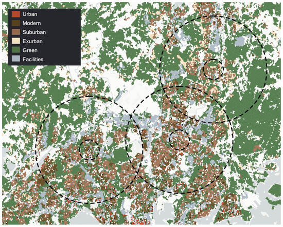
Figure 1.
Land-use as a hexagonal grid with two carbon footprint survey record (CF record) locations, illustrated with a study radii of 1 km and 5 km (dashed lines). Similar-sized land-use hexagons for each classified type were summed for each CF record for 1 km and 5 km correlation analyses. See the Supplementary Materials (Figure S1) for a more detailed illustration.
With land-use reclassification (Table 1), we sought to define categories which had similarities with the typical land-use planning designations used in Nordic zoning while retaining certain generality within a sample of the case cities. Urban Atlas classes are already slightly aligned with land-use planning zoning logic, as they combine density-based classes with functionality-based classes. In zoning-based planning practice, it is typical to apply separate designations for residential building types that differ by their density (e.g., zone for apartment buildings vs. a zone for single-family houses), as well as designations for urban functions like commercial and recreational areas [55]. This approach was chosen to reflect the analysis towards legislative plan-making in Nordic countries. With this setting, we wished to establish conceptual linkages on how empirical insights from the existing environment can inform how planning decisions may influence the carbon footprints of citizens in future.

Table 1.
Classification for land-use. More information about original classification can be found in the Urban Atlas Mapping Guide [54].
2.3. Statistical Method
The selected statistical method was the result of an exhaustive Exploratory Data Analysis (EDA) phase in which we tested multiple different re-classifications, neighbourhood sizes, and statistical approaches. We ran both Spearman and Pearson methods separately on each land-use class and relevant combinations, as well as in the same model. This was repeated on different neighbourhood sizes between 1 km and 9 km radii. As the methods began to repeat similar patterns between the same domains and land-use classes in similar radii, we ended up combining them and focusing on a close range of 1 km while using a 5 km radius for comparison to illustrate the direction of change. On a larger regional scale, the reasons behind land-use types and their distribution around each record are much more diverse and harder to reflect on the operational level of urban planning. We used all the cities as a single sample to keep statistical significance as high as possible while acknowledging certain differences in topography between Nordic capitals. From the findings gathered in the EDA phase, we decided to measure both the Pearson and Spearman as partial correlations between the coverage of different land-use types, measured as equal-sized hexagons (~one hectare each) in the neighbourhood and the carbon footprints of target domains. Using a partial correlation method, we focused the analysis more coherently on our research question and excluded the possible confounding impacts of land-use types. Furthermore, in all the models, we included income (measured in income deciles in each country) and household type (divided into single households, couples, single-parent households, and couples with children) as control variables to avoid biases related to these socio-economic characteristics and to reveal the impacts attributable to the land-use types. By using both Spearman and Pearson methods, we ensured that we did not miss nonlinear dynamics if the relationship was not straight but was still consistent in direction.
Before conducting the partial correlation calculations, we assigned a default minimum value of 1 kg of yearly carbon to any records containing null or zero values for target carbon footprints. This approach allowed us to include all records in all calculations. This prevented, for example, the correlations between vehicle footprints and land-use types from being calculated solely among car owners while remaining insignificant as a share in yearly carbon footprints counted in hundreds of CO2e kg. Accordingly, we replaced zero values with 1.0 for land-use types that were completely missing in the study radii of some records. Similarly to footprints, the one hexagon addon remains insignificant as a share in land-use type sums within the studied neighbourhood radii, in which sum values for each land-use type hexagon are counted in hundreds in a 1 km radius and thousands in a 5 km radius. These add-ons were an application of a fix introduced by Bellégo et al. [56] to avoid infinity errors in natural logarithmic transformation. Applying Bellego’s fix was essential to maximise the sample size and ensure high data integrity for our partial correlation analysis. This allowed us to generate statistically comparable values for each pair of variables. Critically, it prevented the need to exclude entire data records due to localised missing values—for example, avoiding the situation where records are skipped because vehicle values would be zero. This ensured that every available measurement point contributed to the analysis, making our resulting correlations statistically more reliable and truly comparative across all tested pairs.
After this, the distributions of all features were logarithmically transformed before the calculation of partial correlation to make the scales comparable and distributions more normal. As the primary goal here was not precise statistical inference in the classical sense, but rather to understand the direction and relative strength of the associations between different land-use types and individual carbon footprints in the open system of a city, the detailed residual diagnostics were not examined. All partial correlation calculations were done with the Pingouin scientific statistical library for Python [57].
Due to the logarithm transformations, the interpretation of the r value is a percentage change in the given footprint following a one percent unit (hexagon) change in the land-use variable. For example, the r value of −0.1 between Y type footprint and X land-use type indicates that adding, for example, 10 hectares of X land-use coverage within the radius of neighbourhood will decrease (-) inhabitants’ Y type footprint 10 × 0.1 = 1.0 percent. Figure 2 visualises this workflow. Information about the variables used in the statistical analysis, including information about their distributions and confidence intervals, is provided in the Supplementary Materials (File S2_statistical_metrics).
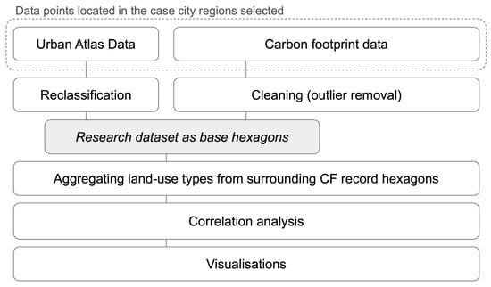
Figure 2.
Workflow phases in this study. CF data points were selected within a 30 km radius, cleaned of outliers to focus on the trend, and then combined with zoning-reclassified land-use data using an additional 10 km buffer. This yielded a research dataset that was used in correlation analysis by aggregating the surrounding land-use context for each CF data point across different radii.
3. Results
To put the land-use impact results into a proper context, we first establish the footprint levels in the five case cities and show how they are distributed across the eight domains in Section 3.1. In Section 3.2., we focus on the land-use impacts on the three domains of the “lifestyle footprint”, Goods and services footprint, Leisure travel footprint, and Vehicle footprint, looking at the cities as one combined sample to increase the data points in the statistical analysis.
3.1. Carbon Footprints and Their Distributions in the Five Case Cities
The carbon footprint data points filtered for this study render the following overall view of the case cities: The overall CBCF in the case cities vary from a lowest of 5.5 tCO2e in Stockholm to 7.2 tCO2e in Helsinki, as shown in Figure 3. The key domain behind the differences is Housing due to the much more GHG-intensive stationary energy systems in Finland and Denmark compared to the other countries. However, the second-highest footprints were found in Reykjavik due to high affluence and high vehicle-related emissions. The Goods and services footprints also show significant variation from 0.6 tons in Stockholm to 1.2 tons in Helsinki and Reykjavik; and Leisure travel footprints also show significant variation from 0.5 in Stockholm to 1.3 in Reykjavik.
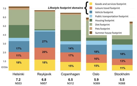
Figure 3.
Carbon footprint per capita (tCO2e/a) in each case-city divided into eight consumption domains. N-figures (e.g., N553) indicate the number of data points in a particular city sample filtered for this study. Percent figures indicate the share of each lifestyle footprint domain within the city. Overall, the lifestyle footprint shares ranges from 42% in Stockholm to 65% in Reykjavik.
3.2. Land-Use Impacts on the “Lifestyle Footprint” Component Domains
Figure 4 visualises correlation trends between target footprints and land-use classes within a 1 km radius using all data points from all cities as a sample. Land-use types on the x-axis are arranged from left to right, beginning with types that are common in denser central areas and progressing toward dominant types that are common in less dense areas. What can be seen is that a higher Goods and services footprint, and especially the Leisure travel footprint, align with the land-use types typical in urban settings (urban, facilities and recreational) while vehicle footprint shows inverted results. Total footprint reflects the pattern of vehicle footprint, resulting in a negative direction with the Urban land-use type. However, the expected mirrored impact for the Vehicle footprint is not recognised with the types typical in edge city region (Suburban, Exurban and Green), even if the impacts on the Goods and services and Leisure travel domains are inverted. An inverted impact for Vehicle footprint is slightly recognised with the Green type, but is accompanied by a non-inverted impact on Goods and services. The Green type dominates, especially in the neighbourhoods beyond the edge city zone, but also in the suburban areas, which are often located next to green corridors and inner-city zones in Nordic capital cities (e.g., Copenhagen’s famous finger plan and its adaptations).
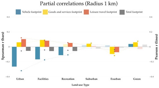
Figure 4.
Partial Spearman correlation levels (colour bars) and Pearson regression slope beta-values (lines) for target carbon footprints per land-use type (x-axis) in a 1 km radius in target Nordic capitals (N 2559). Insignificant values (p > 0.05) are greyed out.
The context changes when correlations are calculated using land-use types summed from a larger 5 km radius (Figure 5). In a 5 km radius, the distribution of reachable land-use types changes considerably, rendering a view in which non-urban types (Suburban, Exurban, Green) dominate most locations. Most likely because of this reason, the direction of the impact of most types is negative for Vehicle footprints and positive for Goods and services and Leisure travel. This may indicate the general effect of the urban environment, as all our records are inside the capital city regions: everything is accessible within a 5 km radius. The lower values for Urban land-use type illustrate the same phenomenon, as the most dense Urban land-use is underrepresented in a 5 km radius, even in central locations; City centres of Nordic capital cities are not very large geographically.
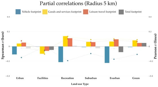
Figure 5.
Partial Spearman correlation levels (colour bars) and Pearson regression slope beta-values (lines) for target carbon footprints per land-use type (x-axis) in a 5 km radius in target Nordic capitals (N 2559). Insignificant values (p > 0.05) are greyed out.
Due to the log-log transformation, as well as the different nature of the units of variables, low partial correlations (r) are expected. Unlike traditional interpretations where r values closer to ±0.5 indicate a moderate correlation, in this setup, smaller values also signify a pattern, especially if both Spearman and Pearson have similar directions. If Spearman is high but Pearson is low, this suggests that the relationship exists but is nonlinear. If Spearman is low while Pearson is high, this indicates that the relationship is not consistent across data points. In our analysis, all footprint–land-use pairs render similar direction results for Spearman and Pearson, indicating that recognised correlations are somewhat linear and consistent. The values that are similar in direction while also significant (e.g., Urban land-use impact on Vehicle footprint) indicate that the particular land-use type might have a causal power (in Critical Realism terms) on the given carbon footprint domain of the residents in that neighbourhood.
4. Discussion
It is well established that lifestyles change significantly along the urban–rural continuum. However, there is limited research on the extent to which land-use patterns at the neighbourhood scale influence these outcomes, especially given that commercial services in cities are generally accessible to all within relatively short distances. This is the research gap we are approaching here by using Nordic capitals as case data with results from a carbon footprint survey [16] combined with within urban area land-use classification derived from Urban Atlas [54]. Moreover, we see that climate change is one of the most pressing threats to humanity, with urban development and construction as key drivers. We therefore approach the results not merely as empirical observations of the past, but as insights to inform urban planning practices that shape the foundation for similar impacts in the future. Hence, we reflect the results, especially on the legislative plan-making action, which defines the type of development using zoning plans. These plans ultimately lead to the land-use types that are tracked in the datasets, like the Urban Atlas data used here. From this perspective, we are ultimately interested in whether there is any indication of a correlation between the locally zoned land-use types and lifestyle carbon footprints of the residents.
Before delving into the nexus of the study, we established the full footprint levels in the case cities and the distributions across the domains to which the footprint calculations were split. We found that the footprints vary from 5.5 tons per capita in Stockholm to 7.2 tons per capita in Helsinki, with the “lifestyle footprint” component, Goods and services, Leisure travel, and Vehicle footprint, explaining ±50%, but with significant variation across the cities.
As the next step, we focused on the land-use impact on the three “lifestyle footprint” domains. The results of this analysis confirm that, within a close range (1 km), there is a positive correlation between urban land-use and Goods and services, as well as Leisure travel, whereas Vehicle footprint correlates negatively. This outcome aligns well with previous research. However, our novel finding is that this well-established pattern is not inversely reflected in the low-density land-use types (Suburban, Exurban, and Green). Contrary to our expectations, these low-density environments inside and on the edge of the city did not show a positive correlation with the Vehicle footprint. Interestingly, when expanding the analysis to a 5 km radius, the Exurban land-use type specifically showed a clearly negative correlation with the Vehicle footprint in both Spearman and Pearson values—a relationship that was not observed in the 1 km study.
In a 5 km radius, the Vehicle footprint impact of the Exurban type is both consistent and linear, which is not the case with the Suburban type. This may indicate that the largest carbon footprints occur in middle-level suburban environments, but in highly exurban environments (measured within a 5 km radius), people may drive infrequently and consume less overall per unit time, resulting in a similar negative direction with the Total footprint. Like in the 1 km study, also in the 5 km radius, the impact of Green type is most likely mixed with suburban areas, which are mostly located next to green corridors in Nordic cities and hence render different influences than Exurban type. The similar patterns between Green and Suburban land-use types also indicate this. The deviant pattern related to Facility land-use type in a 5 km radius stems most likely from a variety of industrial land usage inside that type. Facility land-use types also consist of commercial clusters, which are sparse in numbers and highly concentrated, resulting in a loose network in Nordic cities [12,58]. The impact of retail centres is probably hidden in the varying mix of industrial land-uses, as these different types are gathered under one class in the original Urban Atlas data.
While our results between urban land-use types and target carbon footprint domains mostly align clearly with the earlier research findings, the notion that urban impact is not inverted with the Exurban land-use but actually renders a significant negative direction within a 5 km radius is a new finding. This may indicate the differences in the consumption intensity of the lifestyles [16], meaning that while a car is the default mode of transport in exurban locations, it is probably not used so frequently if the distance to services gets longer, as its difference with the suburban type indicates. This may also hinder the rise in the Total footprint, which also renders a negative direction in exurban environments.
The negative correlation between Exurban land-use and the Goods and services footprint observed in a 1 km study indicates lower consumption at more exurban locations, whereas the same correlation is positive in a 5 km study, while the Total footprint remains negative. This divergent finding suggests that part of the positive Goods and services footprint correlation in Exurban locations in a 5 km study is due to the mixed impact. Some data points located in the inner-city locations without nearby Exurban land-use are still catching exurban types far around them and impacting the 5 km study results. Otherwise, a 1 km study would render similar results with the Goods and services footprint. These results suggest that, despite the dominance of vehicle use among transport modes in Exurban locations, the characteristics of Exurban land-use are associated with a lower total lifestyle footprint, which most likely stems from lower consumption levels in time. This interpretation is a hypothesis that aligns with more coarse previous studies we have referred to in the Introduction (e.g., [23,25,27,29]).
Similarly, the correlations in the most Urban locations ease off when calculating land-use within a 5 km radius. In this sense, suburban living will probably balance between the urban–rural continuum as it has no clear impact in either direction in this scope. This may also indicate the mixed impacts of suburbs, combining the carbon-intensive drawbacks of both urban consumption and rural travel modes. Research in the U.S. context using econometric models on household carbon footprints (including housing energy) has found that the sheer scale of American suburbanization offsets the mobility GHG benefits of urban cores, leading to higher overall net emissions in large metropolitan areas compared to smaller ones [31]. However, the results depend heavily on the scope of analysis. In Canada, a study applying Life Cycle Assessment to compare low- and high-density residential areas has found that changing the functional unit in the assessments from per capita to the unit of living space will remove the benefits of density [59]. Similarly, when considering the city scale, Jones et al. did not find any net GHG benefits of urban density [31]. Even when only focusing on mobility and housing energy footprints, scholars have found the impact of density to be moderate [60]. These findings may stem from the consumerist lifestyle, which planning is expected to support in central locations. In addition, in Germany, scholars have concluded that the high share of single households with greater consumption opportunities in city centres is one of the main reasons mobility and energy per capita benefits are reset, resulting in cities of different sizes and densities being more or less on par in terms of per capita emissions [61]. Also, when focusing solely on commuting coming outside the city centres, the results reveal similar spatial heterogeneity and nonlinearity in the impact of the built environment [62,63]. These divergent results illustrate the difficulty of deriving a holistic figure of impacts when using a per capita approach with density. Per capita assessments, especially when applied without indirect impacts, easily favour density, as population or GFA figures are used as dividers in the equations. In addition, the cultural context challenges these calculations. For example, unlike in Europe or North America where geography seems to act as a spatial differentiator of emissions, the Chinese context shows that the general transition into the consumer-oriented urban middle class itself is the primary vector for explosive carbon footprint growth of cities [25]. These comparative perspectives reveal that the measured GHG impact of zoning depends on the scope and the unit used in the analysis. They also illustrate that the actual net impact is highly context-dependent and dominated by the indirect impacts. Achieving deep decarbonization requires planners to acknowledge that “compactness” is not a universal cure; plans must be tailored to mitigate the specific high-emission behaviours that cultural and structural environments provoke. It is doubtful that the city’s emissions can ever be fully assessed as a commensurate numerical metric. Considering that the prime goal of the assessments is to help us to mitigate urban development by finding a less harsh design, the direction, not the precise figure, may be more fruitful to assess holistically.
These notions call for more detailed research to be conducted on different urban environment details and using a longitudinal dataset like anonymised mobile phone data to get a more detailed view of the lifestyle impacts facilitated by urban planning. Using the longitudinal data of carbon footprints and well-classified, detailed spatial data of the environment might overcome the limitations related to the datasets used in this study. Limitations stemming from Urban Atlas categories arise from the influential role of classifications in correlation analyses. Urban Atlas provides consistent classification, which aligns well with European zoning traditions. To increase contextual validity in research, we applied zoning-related reclassifications and resolutions relevant to zoning plan-making when aggregating surrounding data on carbon footprint record points for correlation calculations. Using different data sources with different classifications would yield different results and disrupt the connection in this research context. Urban Atlas provided the best available commensurate data within the Nordic coverage, as the classification aligns with land-use planning zoning logic, combining density-based classes with functionality-based classes, as zoning plans do.
Another limitation of this study relates to the scope in which the emissions were included and analysed. While we purposefully focused on the lifestyle footprints, it is important to notice that the results should also be interpreted within that scope. All urban development, which shapes the lifestyle footprints, causes emissions, and these emissions can be extremely high. Rankin et al. [64] recently estimated that construction emissions alone could use up the whole carbon budget left for the 2 °C climate target by 2030. As these emissions vary between land-use types, future studies should include or even focus on them and their associations with land-use in within-urban settings.
Another precision issue relates to the carbon footprint calculations. Regarding local mobility, we asked the survey respondents to estimate the weekly distance travelled with different modes of transport. This is prone to estimation errors, particularly among people living within the same urban area (compared to broader comparisons across the urban–rural continuum). Comparisons to mobility data collected with, for example, mobile phones, reflecting the actual mobility, would be interesting and valuable. Similarly, the Goods and services footprint was calculated based on the spending estimations of the respondents across aggregated consumption domains. This again makes the calculations prone to estimation errors, but they also suffer from the inherent input–output method problem of linearity between monetary values and emissions. It is also possible that the correlations relate to underlying socio-economic factors instead of land-use per se. This possibility cannot be fully ruled out. Therefore, a more detailed approach combined with a bottom-up footprint calculation method would be a valuable step forward.
Finally, an online data collection method focusing mainly on social media might lead to non-representativeness of the sample. As we discussed in Section 2, representativeness was not aimed at, but instead our target was to capture a wide variety of lifestyles. However, some steering of the social media advertisement campaign was done by the company executing the campaign regarding selected socio-economic variables. Still, the final sample contains socio-economic biases towards females and high education level. Future studies should repeat a similar land-use analysis using representative samples. The data collection method also returns a cross-sectional dataset, which limits our ability to detect causal relationships between urban form and carbon footprints.
Regardless of these limitations and uncertainties, the findings of this study are suggestive evidence of the Critical Realist’s concept of causal power, which land-use planning can have on urban lifestyles, as Naess has suggested [38]. Divergent results from embodied per capita, per-GFA, and lifestyle-based sustainability analyses of urban structures present a significant research theme yet to be addressed. Future research frameworks must deconstruct these conflicting perspectives into comparable data, ideally examined through Critical Realism, to integrate underlying drivers such as real estate economics with countervailing forces such as urban biodiversity and ecosystem service needs.
5. Conclusions
The causal power of land-use planning should be leveraged to facilitate much-needed systemic change toward less-carbon-intensive urban development and lifestyles, both of which the public sector is expected to support [20]. If we manage to fine-tune the local neighbourhood-level impacts downward, we may achieve considerable city-level impact, thereby aggregating carbon-neutrality goals at the national and global levels. In this scenario, fewer goods are consumed, and less steel and concrete are used for less compact city infrastructure. This can be seen as a green transition for planning, but also for new urban economics, rather than a nihilist view of the end of cities.
To learn to leverage urban design for climate mitigation in more detail is an important New School for planning practice, as well as for planning theory research. Our results, especially the differences between the 1 km and 5 km studies, show that small-scale local solutions for land-use might have an impact, but that this impact can be overshadowed by the regional structure. The use of the legal power of urban plans to influence functional patterns in cities to avoid negative impacts has a strong historical background. Urban planning as a profession emerged to reduce the negative impacts of urban density, which led to the development of theories to promote themes as openness and functional decentralisation as practical solutions (see, e.g., [6,18,65]). By the turn of the 21st century, the goals of urban planning had inverted in that sense. This inversion has led to a lock-in situation in the development of low-carbon construction methods: most of the contemporary capabilities and innovations can not be applied, as urban plans have too high efficiency for too large buildings, in which the use of less-carbon-intensive materials and site usage is no longer possible [66]. To unlock the situation, the planners need to re-learn to apply land-use decentralisation to manage the city’s growth: not by infilling it only in the centres with high volumes, but by balancing it regionally. The popular 15 min city concept encompasses this perspective, even if it is often used as a synonym for the compact city paradigm. The “Ville du quart d’heure” initiative, championed by Paris Mayor Anne Hidalgo, is a leading example of urban planning focused on decentralising city services and prioritising sustainable infrastructure in these new local hubs [67]. But, as with the impacts of density in zoning, it clearly seems that also polycentrism—the key to healthy local development—in the concept of the 15 min city must find its localised format for the “nudge” towards lower urban emissions [68].
Our study’s evidence regarding the causal power of urban plans, coupled with the Parisian example, suggests a renewed appreciation for the impacts of physical plans to manage urban development. This emerging focus is also recognised by planning theorists, pointing out how it involves integrating traditional urban planning principles, rooted all the way back to the foundational work of Patrick Geddes—the father of the profession—with contemporary cutting-edge technological analytical capabilities [69]. The climate change perspective and impact-based urban plan-making, accordingly, presents urban planners with the opportunity to renew their field significantly by utilising both their own professional history and the latest science and technology. Fundamental question deals with the raison d’être and mandate of urban planning institutions in the climate of the 21st century.
Supplementary Materials
The following supporting information can be downloaded at https://www.mdpi.com/article/10.3390/environments13030173/s1. Calculation method description (File S1) [42,43,44,45,46,47,48,50,51,52,53,70,71,72,73,74,75,76,77,78,79,80,81,82,83,84,85]; Figure S1: Detailed explanation of Figure 1; File S2_statistical_metrics: Information about variable distributions across 1 and 5 km ranges.
Author Contributions
Conceptualization, T.J.; methodology, T.J. and J.H.; spatial analysis, T.J.; validation and data curation, T.J., J.H. and H.T.; writing, T.J. and J.H.; review, H.T.; visualisations, T.J. All authors have read and agreed to the published version of the manuscript.
Funding
This research was funded by the Science Park of University of Iceland, and by the Icelandic Centre for Research RANNIS (grant number 207195-052).
Institutional Review Board Statement
Ethical review and approval were waived for this study due to the anonymous and non-sensitive nature of the online survey, with voluntary participation.
Informed Consent Statement
Informed consent was obtained from all subjects involved in the study.
Data Availability Statement
The original data presented in the study are openly available in Zenodo at https://zenodo.org/records/10656970 (accessed on 1 May 2025).
Acknowledgments
The authors thank the Science Park of University of Iceland the Icelandic Centre for Research RANNIS for funding the study. The authors made use of geocomputing resources provided by the Open Geospatial Information Infrastructure for Research (Geoportti, urn:nbn:fi:research-infras-2016072513) funded by the Research Council of Finland, CSC—IT Center for Science, and other Geoportti consortium members.
Conflicts of Interest
The authors declare no conflicts of interest.
Abbreviations
The following abbreviations are used in this manuscript:
| CFBC | Consumption-Based Carbon Footprints |
| CF | Carbon Footprint |
| CO2e | Carbon dioxide equivalent |
| COICOP | Classification of Individual Consumption According to Purpose |
| EDA | Exploratory Data Analysis |
| FUA | Functional Urban Areas |
| GHG | Greenhouse Gas |
| GFA | Gross Floor Area |
| IPCC | Intergovernmental Panel on Climate Change |
| IQR | Interquartile Range |
| MMU | Minimum Mapping Unit |
| TOD | Transit Oriented Development |
References
- Pont, M.B.; Haupt, P.; Berg, P.; Alstäde, V.; Heyman, A. Systematic review and comparison of densification effects and planning motivations. Build. Cities 2021, 2, 378. [Google Scholar] [CrossRef]
- Boulange, C.; Gunn, L.; Giles-Corti, B.; Mavoa, S.; Pettit, C.; Badland, H. Examining associations between urban design attributes and transport mode choice for walking, cycling, public transport and private motor vehicle trips. J. Transp. Health 2017, 6, 155–166. [Google Scholar] [CrossRef]
- Cervero, R.; Kockelman, K. Travel demand and the 3Ds: Density, diversity, and design. Transp. Res. Part D Transp. Environ. 1997, 2, 199–219. [Google Scholar] [CrossRef]
- Dovey, K.; Pafka, E. What is walkability? The urban DMA. Urban Stud. 2020, 57, 93–108. [Google Scholar] [CrossRef]
- Heroy, S.; Loaiza, I.; Pentland, A.; O’Clery, N. Are neighbourhood amenities associated with more walking and less driving? Yes, but predominantly for the wealthy. Environ. Plan. B Urban Anal. City Sci. 2023, 50, 958–982. [Google Scholar] [CrossRef]
- Batty, M.; Marshall, S. Centenary paper: The evolution of cities: Geddes, Abercrombie and the new physicalism. Town Plan. Rev. 2009, 80, 551–574. [Google Scholar] [CrossRef]
- Ferreira, A.C.; Batey, P. On Why Planning Should Not Reinforce Self-Reinforcing Trends: A Cautionary Analysis of the Compact-City Proposal Applied to Large Cities. Environ. Plan. B-Plan. Des. 2011, 38, 231–247. [Google Scholar] [CrossRef]
- Priyadarshi, S.; Skea, J.; Reisinger, A. Mitigation of Climate Change—Working Group III Contribution to the WGIII Sixth Assessment. Report of the Intergovernmental Panel on Climate Change, Climate Change. 2022. Available online: https://www.ipcc.ch/report/ar6/wg3/downloads/report/IPCC_AR6_WGIII_FullReport.pdf (accessed on 23 April 2025).
- UN Habitat. A New Strategy of Sustainable Neighbourhood Planning: Five Principles (Discussion Note 3). UN Habitat. 2014. Available online: https://unhabitat.org/sites/default/files/documents/2019-05/five_principles_of_sustainable_neighborhood_planning.pdf (accessed on 23 April 2025).
- Berghauser Pont, M.; Haupt, P. Spacematrix: Space, Density and Urban Form; nai010 Publishers: Rotterdam, The Netherlands, 2021. [Google Scholar]
- Czepkiewicz, M.; Heinonen, J.; Ottelin, J. Why do urbanites travel more than do others? A review of associations between urban form and long-distance leisure travel. Environ. Res. Lett. 2018, 13, 073001. [Google Scholar] [CrossRef]
- Culley, J. An Empirical Investigation into the Changes in the Grocery Retailing Landscape—A Helsinki Metropolitan Region Case Study. Ph.D. Thesis, Aalto University, Espoo, Finland, 2020. Available online: http://urn.fi/URN:ISBN:978-952-60-8968-3 (accessed on 24 December 2024).
- Jama, T.; Henrikki, T.; Henrik, L.; Anssi, J. Compact city and urban planning: Correlation between density and local amenities. Environ. Plan. B Urban Anal. City Sci. 2024, 52, 44–58. [Google Scholar] [CrossRef]
- Heinonen, J.; Jalas, M.; Juntunen, J.K.; Ala-Mantila, S.; Junnila, S. Situated lifestyles: I. How lifestyles change along with the level of urbanization and what the greenhouse gas implications are—A study of Finland. Environ. Res. Lett. 2013, 8, 025003. [Google Scholar] [CrossRef]
- Dawkins, E.; Rahmati-Abkenar, M.; Axelsson, K.; Grah, R.; Broekhoff, D. The carbon footprints of consumption of goods and services in Sweden at municipal and postcode level and policy interventions. Sustain. Prod. Consum. 2024, 52, 63–79. [Google Scholar] [CrossRef]
- Heinonen, J.; Olson, S.; Czepkiewicz, M.; Árnadóttir, Á.; Ottelin, J. Too much consumption or too high emissions intensities? Explaining the high consumption-based carbon footprints in the Nordic countries. Environ. Res. Commun. 2022, 4, 125007. [Google Scholar] [CrossRef]
- Carta, S. (Ed.) Machine Learning and the City: Applications in Architecture and Urban Design, 1st ed.; Wiley: Hoboken, NJ, USA, 2022. [Google Scholar] [CrossRef]
- Bruegmann, R. Sprawl: A Compact History; University of Chicago Press: Chicago, IL, USA, 2005. [Google Scholar] [CrossRef]
- Bhaskar, R. (Ed.) Interdisciplinarity and Climate Change: Transforming Knowledge and Practice for Our Global Future; Routledge: London, UK, 2010. [Google Scholar] [CrossRef]
- Salo, M.; Heiskanen, E.; Heikkinen, M.; Heinonen, T. Ohjauskeinoja Kotitalouksien Kulutuksen Hiilijalanjäljen Pienentämiseen. 2023. Available online: https://julkaisut.valtioneuvosto.fi/handle/10024/165085 (accessed on 23 April 2025).
- Creutzig, F.; Niamir, L.; Bai, X.; Callaghan, M.; Cullen, J.; Díaz-José, J.; Figueroa, M.; Grubler, A.; Lamb, W.F.; Leip, A.; et al. Demand-side solutions to climate change mitigation consistent with high levels of well-being. Nat. Clim. Change 2022, 12, 36–46. [Google Scholar] [CrossRef]
- Thaler, R.H.; Sunstein, C.R. Nudge: The Final Edition (Updated Edition); Penguin Books, an Imprint of Penguin Random House LLC: London, UK, 2021. [Google Scholar]
- Ottelin, J.; Ala-Mantila, S.; Heinonen, J.; Wiedmann, T.; Clarke, J.; Junnila, S. What can we learn from consumption-based carbon footprints at different spatial scales? Review of policy implications. Environ. Res. Lett. 2019, 14, 093001. [Google Scholar] [CrossRef]
- Anttonen, H.; Kinnunen, A.; Heinonen, J.; Ottelin, J.; Junnila, S. The spatial distribution of carbon footprints and engagement in pro-climate behaviors—Trends across urban-rural gradients in the nordics. Clean. Responsible Consum. 2023, 11, 100139. [Google Scholar] [CrossRef]
- Wiedenhofer, D.; Guan, D.; Liu, Z.; Meng, J.; Zhang, N.; Wei, Y.-M. Unequal household carbon footprints in China. Nat. Clim. Change 2017, 7, 75–80. [Google Scholar] [CrossRef]
- Reichert, A.; Holz-Rau, C.; Scheiner, J. GHG emissions in daily travel and long-distance travel in Germany—Social and spatial correlates. Transport. Res. Part D Transp. Environ. 2016, 49, 25–43. [Google Scholar] [CrossRef]
- Chen, S.; Liu, Z.; Chen, B.; Zhu, F.; Fath, B.D.; Liang, S.; Su, M.; Yang, J. Dynamic Carbon Emission Linkages Across Boundaries. Earth’s Future 2019, 7, 197–209. [Google Scholar] [CrossRef]
- Heinonen, J.; Junnila, S. A Carbon Consumption Comparison of Rural and Urban Lifestyles. Sustainability 2011, 3, 1234–1249. [Google Scholar] [CrossRef]
- Ala-Mantila, S.; Ottelin, J.; Heinonen, J.; Junnila, S. To each their own? The greenhouse gas impacts of intra-household sharing in different urban zones. J. Clean. Prod. 2016, 135, 356–367. [Google Scholar] [CrossRef]
- Shi, W.; Goodchild, M.F.; Batty, M.; Kwan, M.-P.; Zhang, A. Urban Informatics; Springer: Singapore, 2021. [Google Scholar] [CrossRef]
- Jones, C.; Kammen, D. Spatial distribution of U.S. Household carbon footprints reveals suburbanization undermines greenhouse gas benefits of urban population density. Environ. Sci. Technol. 2014, 48, 895–902. [Google Scholar] [CrossRef] [PubMed]
- Zhu, K.; Tu, M.; Li, Y. Did Polycentric and Compact Structure Reduce Carbon Emissions? A Spatial Panel Data Analysis of 286 Chinese Cities from 2002 to 2019. Land 2022, 11, 185. [Google Scholar] [CrossRef]
- Creutzig, F.; McPhearson, T.; Bardhan, R.; Belmin, C.; Chow, W.T.L.; Garschagen, M.; Hsu, A.; Kılkış, Ş.; Islam, S.T.; Milojevic-Dupont, N.; et al. Bridging the scale between the local particular and the global universal in climate change assessments of cities. Nat. Cities 2025, 2, 369–378. [Google Scholar] [CrossRef]
- Ala-Mantila, S.; Heinonen, J.; Clarke, J.; Ottelin, J. Consumption-based view on national and regional per capita carbon footprint trajectories and planetary pressures-adjusted human development. Environ. Res. Lett. 2023, 18, 024035. [Google Scholar] [CrossRef]
- Müller, D.B.; Liu, G.; Løvik, A.N.; Modaresi, R.; Pauliuk, S.; Steinhoff, F.S.; Brattebø, H. Carbon Emissions of Infrastructure Development. Environ. Sci. Technol. 2013, 47, 11739–11746. [Google Scholar] [CrossRef]
- Tian, P.; Zhong, H.; Chen, X.; Feng, K.; Sun, L.; Zhang, N.; Shao, X.; Liu, Y.; Hubacek, K. Keeping the global consumption within the planetary boundaries. Nature 2024, 635, 625–630. [Google Scholar] [CrossRef]
- Bhaskar, R. A Realist Theory of Science; Routledge: London, UK, 2008. [Google Scholar] [CrossRef]
- Næss, P. Built environment, causality and urban planning. Plan. Theory Pract. 2016, 17, 52–71. [Google Scholar] [CrossRef]
- Girod, B.; de Haan, P. More or better? A model for changes in household greenhouse gas emissions due to higher income. J. Ind. Ecol. 2010, 14, 31–49. [Google Scholar] [CrossRef]
- André, M.; Bourgeois, A.; Combet, E.; Lequien, M.; Pottier, A. Challenges in measuring the distribution of carbon footprints: The role of product and price heterogeneity. Ecol. Econ. 2024, 220, 108122. [Google Scholar] [CrossRef]
- Leferink, E.; Heinonen, J.; Ala-Mantila, S.; Árnadóttir, Á. Climate concern elasticity of carbon footprint. Environ. Res. Commun. 2023, 5, 075003. [Google Scholar] [CrossRef]
- Stadler, K.; Wood, R.; Bulavskaya, T.; Södersten, C.J.; Simas, M.; Schmidt, S.; Usubiaga, A.; Acosta-Fernández, J.; Kuenen, J.; Bruckner, M.; et al. EXIOBASE 3: Developing a Time Series of Detailed Environmentally Extended Multi-Regional Input-Output Tables. J. Ind. Ecol. 2018, 22, 502–515. [Google Scholar] [CrossRef]
- Ottelin, J.; Cetinay, H.; Behrens, P. Rebound effects may jeopardize the resource savings of circular consumption: Evidence from household material footprints. Environ. Res. Lett. 2020, 15, 104044. [Google Scholar] [CrossRef]
- Aamaas, B.; Borken-Kleefeld, J.; Peters, G.P. The climate impact of travel behavior: A German case study with illustrative mitigation options. Environ. Sci. Policy 2013, 33, 273–282. [Google Scholar] [CrossRef]
- VTT. (n.d.). LIPASTO Unit Emissions-Database [Dataset]. Available online: https://lipasto.vtt.fi/yksikkopaastot/ (accessed on 16 June 2021).
- Chester, M.V.; Horvath, A. Environmental assessment of passenger transportation should include infrastructure and supply chains. Environ. Res. Lett. 2009, 4, 024008. [Google Scholar] [CrossRef]
- Cherubini, F.; Bird, N.D.; Cowie, A.; Jungmeier, G.; Schlamadinger, B.; Woess-Gallasch, S. Energy- and greenhouse gas-based LCA of biofuel and bioenergy systems: Key issues, ranges and recommendations. Resour. Conserv. Recycl. 2009, 53, 434–447. [Google Scholar] [CrossRef]
- Dillman, K.J.; Árnadóttir, Á.; Heinonen, J.; Czepkiewicz, M.; Davíðsdóttir, B. Review and meta-analysis of EVs: Embodied emissions and environmental breakeven. Sustainability 2020, 12, 9390. [Google Scholar] [CrossRef]
- Heinonen, J.; Ottelin, J.; Ala-Mantila, S.; Wiedmann, T.; Clarke, J.; Junnila, S. Spatial consumption-based carbon footprint assessments—A review of recent developments in the field. J. Clean. Prod. 2020, 256, 120335. [Google Scholar] [CrossRef]
- Saarinen, M.; Kaljonen, M.; Niemi, J.; Antikainen, R.; Hakala, K.; Hartikainen, H.; Heikkinen, J.; Joensuu, K.; Lehtonen, H.; Mattila, T.; et al. Effects of Dietary Change and Policy Mix Supporting the Change—End Report of the FoodMin Project (No. 2019:47; Publications of the Governments’ Analysis, Assessment and Research Activities); Prime Minister’s Office: Helsinki, Finland, 2019. [Google Scholar]
- Ottelin, J.; Heinonen, J.; Junnila, S. New Energy Efficient Housing Has Reduced Carbon Footprints in Outer but Not in Inner Urban Areas. Environ. Sci. Technol. 2015, 49, 9574–9583. [Google Scholar] [CrossRef]
- Yavor, K.M.; Lehmann, A.; Finkbeiner, M. Environmental Impacts of a Pet Dog: An LCA Case Study. Sustainability 2020, 12, 3394. [Google Scholar] [CrossRef]
- Herrera-Camacho, J.; Baltierra-Trejo, E.; Taboada-González, P.A.; Fernanda Gonzalez, L.; Marquez-Benavides, L. Environmental Footprint of Domestic Dogs and Cats. Preprints 2017, 2017070004. [Google Scholar] [CrossRef]
- European Environment Agency. Urban Atlas Land Cover/Land Use 2018 (Vector), Europe, 6-Yearly, Jul. 2021, version 01.03; European Environment Agency: Copenhagen, Denmark, 2020. [Google Scholar] [CrossRef]
- ARL, I. Country profiles. In Country Profiles; Leibniz Association: Berlin, Germany, 2025; Available online: https://www.arl-international.com/knowledge/country-profiles (accessed on 23 April 2025).
- Bellégo, C.; Benatia, D.; Pape, L. Dealing with Logs and Zeros in Regression Models (Version 1). arXiv 2022, arXiv:2203.11820. [Google Scholar] [CrossRef]
- Vallat, R. Pingouin: Statistics in Python. J. Open Source Softw. 2018, 3, 1026. [Google Scholar] [CrossRef]
- Smas, L. URBANISATION: Nordic geographies of urbanisation. In State of the Nordic Region 2018; Grunfelder, J., Rispling, L., Norlén, G., Eds.; Nordic Council of Ministers: Copenhagen, Denmark, 2018; pp. 36–46. [Google Scholar] [CrossRef]
- Norman, J.; MacLean, H.L.; Kennedy, C.A. Comparing High and Low Residential Density: Life-Cycle Analysis of Energy Use and Greenhouse Gas Emissions. J. Urban Plan. Dev. 2006, 132, 10–21. [Google Scholar] [CrossRef]
- Muñiz, I.; Dominguez, A. The Impact of Urban Form and Spatial Structure on per Capita Carbon Footprint in U.S. Larger Metropolitan Areas. Sustainability 2020, 12, 389. [Google Scholar] [CrossRef]
- Gill, B.; Moeller, S. GHG Emissions and the Rural-Urban Divide. A Carbon Footprint Analysis Based on the German Official Income and Expenditure Survey. Ecol. Econ. 2018, 145, 160–169. [Google Scholar] [CrossRef]
- Li, Y.; Ye, J.; Li, Z.; Zhu, M.; Li, Y. Impact of built environment on commuting carbon emissions using big data: A case study of Jinan’s main urban area. Sci. Rep. 2025, 15, 16875. [Google Scholar] [CrossRef] [PubMed]
- Guo, L.; Yang, S.; Zhang, Q.; Zhou, L.; He, H. Examining the Nonlinear and Synergistic Effects of Multidimensional Elements on Commuting Carbon Emissions: A Case Study in Wuhan, China. Int. J. Environ. Res. Public Health 2023, 20, 1616. [Google Scholar] [CrossRef] [PubMed]
- Rankin, K.H.; Cabrera Serrenho, A.; Bachmann, C.; Posen, I.D.; Saxe, S. The climate limits of construction in over 1000 cities. Nat. Cities 2026, 3, 115–125. [Google Scholar] [CrossRef]
- Lehnerer, A. Grand Urban Rules; 010 Publishers: Rotterdam, The Netherlands, 2009. [Google Scholar]
- Talvitie, I.; Kinnunen, A.; Amiri, A.; Junnila, S. Can future cities grow a carbon storage equal to forests? Environ. Res. Lett. 2023, 18, 044029. [Google Scholar] [CrossRef]
- Dakouré, A.; Bourdeau-Lepage, L.; Georges, J. The Paris urban plan review: An opportunity to put the 15-Minute City concept into the perspective of the Parisians desire for nature. In Resilient and Sustainable Cities; Elsevier eBooks: Amsterdam, The Netherlands, 2023; pp. 61–75. [Google Scholar] [CrossRef]
- Teixeira, J.F.; Silva, C.; Seisenberger, S.; Büttner, B.; McCormick, B.; Papa, E.; Cao, M. Classifying 15-minute Cities: A review of worldwide practices. Transp. Res. Part A Policy Pract. 2024, 189, 104234. [Google Scholar] [CrossRef]
- LeGates, R.T.; Stout, F. (Eds.) The City Reader, 7th ed.; Routledge: London, UK, 2020. [Google Scholar] [CrossRef]
- Vimpari, J. Should energy efficiency subsidies be tied into housing prices? Environ. Res. Lett. 2021, 16, 064027. [Google Scholar] [CrossRef]
- Statistics Finland. Production of Electricity and Heat. Appendix Table 1. Electricity and Heat Production by Production Mode and Fuel in 2019. Helsinki, Statistics Finland. 2019. Available online: https://www.stat.fi/til/salatuo/2019/salatuo_2019_2020-11-03_tau_001_en.html (accessed on 14 September 2021).
- Karlsdottir, M.R.; Heinonen, J.; Palsson, H.; Palsson, O.P. Life cycle assessment of a geothermal combined heat and power plant basedon high temperature utilization. Geothermics 2020, 84, 101727. [Google Scholar] [CrossRef]
- Euroheat & Power. District Energy in Denmark 2017. 2019. Available online: https://www.euroheat.org/knowledge-hub/district-energy-denmark/ (accessed on 27 September 2021).
- Energi Företagen. Fjärrvärmeproduktion-Fjärrvärmens Bränslemix 2020. 2020. Available online: https://www.energiforetagen.se/energifakta/fjarrvarme/fjarrvarmeproduktion/ (accessed on 23 September 2021).
- Norsk Fjernvarme. Energikilder. Fjernvarme-Energikilder 2020. 2020. Available online: https://www.fjernvarme.no/fakta/energikilder (accessed on 23 September 2021).
- Adato Energia. Kotitalouksien Sähkönkäyttö 2011. Tutkimusraportti 26.2. 2013. Available online: http://www.motiva.fi/files/8300/Kotitalouksien_sahkonkaytto_2011_Tutkimusraportti.pdf (accessed on 17 March 2026).
- Statistics Finland. Dwellings and Housing Conditions. Overview 2019, 2. Household Dwelling Units and Housing Conditions 2019. Helsinki, Statistics Finland. 2019. Available online: http://www.stat.fi/til/asas/2019/01/asas_2019_01_2020-10-14_kat_002_en.html (accessed on 19 August 2021).
- Finnish Energy. Monthly Electricity Statistics. 2019. Available online: https://energia.fi/en (accessed on 3 April 2021).
- Orkustofnun/National Energy Authority of Iceland. Generation of Electricity in Iceland from 1915. 2015. Available online: https://nea.is/the-national-energy-authority/energystatistics/generation-of-electricity/ (accessed on 10 April 2020).
- Danish Energy Agency. Energy Statistics 2019. Available online: https://ens.dk/sites/ens.dk/files/Statistik/energystatistics2019_webtilg.pdf (accessed on 10 May 2021).
- International Energy Agency—IEA. Electricity Generation by Source, Sweden 1990–2019. 2019. Available online: https://www.iea.org/countries/sweden (accessed on 10 May 2021).
- Statistics Norway. Electricity Balance (MWh), by Production and Consumption, Contents and Month. 2020. Available online: https://www.ssb.no/en/statbank/table/12824/ (accessed on 10 May 2021).
- Alhola, K.; Mäenpää, I.; Nissinen, A.; Nurmela, J.; Salo, M.; Savolainen, H. Carbon footprint and raw material requirement of public procurement and household consumption in Finland—Results obtained using the ENVIMAT-model. In Suomen Ympäristökeskuksen Raportteja 15; Nissinen, A., Savolainen, H., Eds.; Finnish Environmental Institute (SYKE): Helsinki, Finland, 2019; p. 33. [Google Scholar]
- United Nations. Classification of Individual Consumption According to Purpose (COICOP) 2018; Statistical Papers. Department of Economic and Social Affairs. Statistics Division. United Nations Publication; Series M No. 99; United Nations: New York, NY, USA, 2018; 265p. [Google Scholar]
- European Central Bank. Statistics. Ecb/Eurosystem Policy and Exchange Rates. Euro Foreign Exchange Reference Rates. 2021. Available online: https://www.ecb.europa.eu/stats/policy_and_exchange_rates/html/index.en.html (accessed on 20 October 2021).


Disclaimer/Publisher’s Note: The statements, opinions and data contained in all publications are solely those of the individual author(s) and contributor(s) and not of MDPI and/or the editor(s). MDPI and/or the editor(s) disclaim responsibility for any injury to people or property resulting from any ideas, methods, instructions or products referred to in the content. |
© 2026 by the authors. Licensee MDPI, Basel, Switzerland. This article is an open access article distributed under the terms and conditions of the Creative Commons Attribution (CC BY) license.