Abstract
In forested regions, transpiration as a main component of evaporation fluxes is important for evaporation partitioning. Physiological behaviours among various vegetation species are quite different. Thus, an accurate estimation of the transpiration rate from a certain tree species needs specific parameterization of stomatal response to multiple environmental conditions. In this study, we chose a 300-m2 beech forest plot located in Vydra basin, the Czech Republic, to investigate the transpiration of beech (Fagus sylvatica) from the middle of the vegetative period to the beginning of the deciduous period, covering 100 days. The sap flow equipment was installed in six trees with varying ages among 32 trees in the plot, and the measurements were used to infer the stomatal conductance. The diurnal pattern of stomatal conductance and the response of stomatal conductance under the multiple environmental conditions were analysed. The results show that the stomatal conductance inferred from sap flow reached the highest at midday but, on some days, there was a significant drop at midday, which might be attributed to the limits of the hydraulic potential of leaves (trees). The response of stomatal conductance showed no pattern with solar radiation and soil moisture, but it did show a clear correlation with the vapour deficit, in particular when explaining the midday drop. The relation to temperature was rather scattered as the measured period was in the moderate climate. The findings highlighted that the parametrization of stress functions based on the typical deciduous forest does not perfectly represent the measured stomatal response of beech. Therefore, measurements of sap flow can assist in better understanding transpiration in newly formed beech stands after bark beetle outbreaks in Central Europe.
1. Introduction
Transpiration is a main component of evaporation fluxes in vegetated areas [1], in particular in the forested region with a dense vegetation cover [2]. A global-scale study indicated that transpiration accounted for 60–80 % of the total evapotranspiration from the land surface [3]. The transpiration process is rather complex and involves the biophysical properties of leaf stomata in response to multiple environmental stresses in terms of the availability of water, carbon, and energy [4]. Transpiration is conducted through the opening leaf stomata, where carbon dioxide (CO2) enters for photosynthesis. This process is supplied by water flux from the deep soil up to the root zone and includes sap flow and root water uptake [5]. The transpiration rates are governed by the physiological behaviour of leaf stomata, which is dictated by the meteorological conditions and soil moisture [6,7].
Quantification of the evapotranspiration rate in forest area is essential in hydrological and ecological studies. The Penman–Monteith equation is the most widely used evapotranspiration model in hydrological studies [8,9]. Hydrologists often use an analytic expression of latent heat fluxes λE (where λ is the latent heat for vaporization, in MJ kg−1) to consider the evapotranspiration system as a single layer (single source) [10]. Many previous studies showed that evapotranspiration calculated with the Penman–Monteith equation can match measurements with a satisfying accuracy in temperate humid areas with a dense vegetation cover [11,12,13]. However, the influence of multiple environmental factors on physiological characteristics varies among vegetation species and the characteristics, therefore, need to be parameterised correctly with regard to a study site.
In general, energy transfer in a soil–vegetation–atmosphere system can be quantified with the electrical analogy method, in which the transpiration rate is dictated with a critical parameter named stomatal conductance (gc, in m s−1) or stomatal resistance (rc = 1/gc, in s m−1) [7,14]. In a forest area, gc for a certain tree species may be quantitatively determined by a traditional method using an inverse calculation of the simplified version of the Penman–Monteith equation using the in situ measured transpiration rate [15]. In the last few decades, sap flow measurement technology has become the most common method to determine transpiration [16]. The measured sap flow rate of individual trees can upscale to an experimental area to provide species-specific transpiration rates, which can be used to inversely estimate the response of gc to multiple environmental stresses during a continuous time span. Kucera et al. [17] used a novel approach where a direct parameterization of the Penman–Monteith equation was developed to compute the diurnal courses of stand canopy conductance from sap flow. Previous studies also showed that the inversely estimated gc commonly shows complex patterns that are intimately related to meteorological variables (i.e., solar radiation, wind speed, the concentration of carbon dioxide in air, air humidity, and temperature), and soil moisture stress [12,18,19,20]. Moreover, the distinct canopy characteristics (e.g., leaf area and leaf morphology) [21,22,23] and stand characteristics (e.g., stand age and structure) [23,24] also affect transpiration.
This study focused on the analysis of leaf stomatal behaviour based on the sap flow experimental data from an ecological changing area under natural disturbance. The study area is located in the upper Vydra basin (Czech Republic). Due to a bark beetle outbreak in the area, the spruce trees (Picea abies) have dried up and trunks have fallen down, and new beech stands (Fagus sylvatica) have been developed from the formal mixed forest stands mainly consisting of spruce and beech trees. Research studies, which have been focused on the bark beetle outbreak at the Šumava Mts., have mainly studied its impact on water regime [25,26,27], water chemistry [28], soil moisture or temperature [29,30], or forest grow after the disturbance [31]. In general, several studies also show changes in the water regime of mixed (spruce/beech) forest [32,33,34] or comparisons between beech and spruce stands [35]. After the forest disturbance, the study area experienced no change or trend of long-term water balance [26], and stream geochemistry changed with long-lasting effects [27]. However, there were detected shifts in the runoff generation processes, mainly in the root zone [27]. For a better understanding of the mechanisms, detailed information on the evapotranspiration process in the area that is undergoing such an intense transition in the vegetation structure is needed.
This research study was thus aimed to assess the evapotranspiration process in the newly formed beech stands in the area affected by bark beetle outbreak. The key research questions were: (i) how to intensively quantify the transpiration rates for a newly formed beech stand in this locality, and (ii) why it is important to evaluate the stomatal behaviour when measuring sap flow.
As far as we know from the literature review, there is no similar study of beech stand transpiration in a location working with a newly formed beech stand as a principal factor of transpiration. A field experiment was set up aimed at the following objectives:
- Quantifying stomatal conductance, gc, of the newly formed beech forest from a vegetative period to a deciduous period;
- Determining the patterns of the diurnal variation of stomatal conductance for different vegetation periods;
- Evaluating the impact of environmental factors on stomatal conductance.
A direct comparison with similar measurements at spruce stands could not be achieved due to the bark beetle outbreak. Therefore, in this study, we conducted a sap flow experiment in a plot covered by beech forest, varying in ages over the middle of summer and the beginning of autumn (day of year DOY 203–302, i.e., 23 July–30 October) in the year of 2015. In situ measurements of sap flow and meteorological forcing variables were used to inversely estimate stomatal conductance, gc.
2. Materials and Methods
2.1. Study Site
The study area (49.0230908 N; 13.4075242 E) was located in an experimental catchment of Rokytka (ROK), in the upper Vydra basin, the headwaters of the Šumava Mts., Czech Republic (Figure 1). The area features a typical mid-latitude montane climate with distinct seasons [27]. The annual mean precipitation is 1370 mm/year and the annual mean air temperature is 3.6 ℃ [26]. The studied area has been affected by extensive spruce forest disturbance resulting from repeated bark beetle outbreaks [36]. As a result, the formerly mixed forest (spruce and beech) has become dominated by beech stands. Our research study has been focused mainly on forest development after the last outbreak. At the study site, the local mixed forest was created mostly by spruce and beech species supplemented by other tree species such as fir (Abies alba), mountain ash (Sorbus aucuparia) or acer (Acer). Due to the forest management in the past, the forest at the study site was mostly by spruce stands or spruce–beech mixed forest stands. After the last bark beetle outbreak, the forest structure contains two dominant elements:
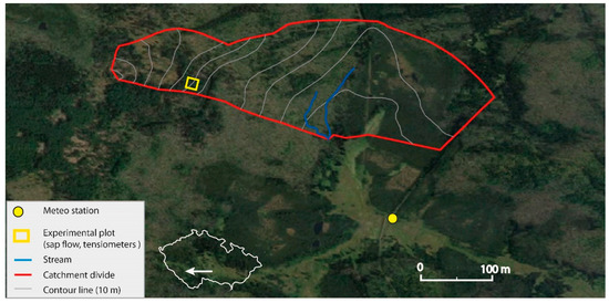
Figure 1.
Location of the study site.
- “Dead” forest stands (at locations with former spruce forests) with grass cover and rarely a solitary tree;
- Beech forests at locations of former mixed forests.
Our study plot belongs to the latter case, and we aimed to observe the transpiration process in such locations after a bark beetle outbreak.
The study site is on a south-facing slope (approximately 3.5°), at an elevation of approximately 1100–1250 m above sea level. The area is covered by dense beech forest (Fagus sylvatica), with blueberries (Vacciniummyrtillus L.) and woodrush (Luzula) at substrate.
Soil was identified as Entic Podzol, with a thin layer (0–8 cm) of organic matter on the top (Figure 2a) [37]. The soil is relatively homogenous based on soil texture analysis (Figure 2b). Due to the granite dominated bedrock, the soil contains only a few clay particles (particle diameter <0.002 mm). Therefore, due to the high content of silt particles (particle diameter = 0.002–0.05), porosity and infiltration rates are rather low. The soil profile has no visible transition between soil, bedrock or water table up to a depth of 20 m below the surface [37].
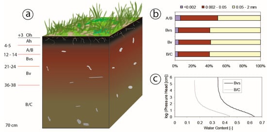
Figure 2.
(a) Sketch of soil condition at different depths in the study plot (unit of depth is cm). (b) Soil layer and soil texture are based on the Czech soil classification: <0.002 mm clay particles, 0.002–0.05 mm slit particles, and 0.05–2 mm sand particles. (c) Water retention curves measured at a depth of 20 cm (Bvs) and 60 cm (B/C) below the surface.
2.2. Experiment Instrumentation and Data
In the study area, a meteorological station (M4016-G, Fielder) at Rokytka (ROK) operated by Charles University in Prague (CUNI) captured data on precipitation, air temperature, net radiation (calculated by the energy balance among the incoming and outgoing shortwave and longwave irradiance), wind speed, and relative air humidity with 10-min intervals. Two tensiometers (T8 Tensiometer, UMS) at the study site measured soil pore water pressure and soil temperature at depths of 20 cm and 60 cm in the soil with 30-min interval (Figure 3a). Water retention curves at two depths were measured in the lab using a pressure plate extractor (1500F1—Soil Moisture Comp.) and created in RETC software using van Genuchten´s formula [38], visible in Figure 2c.
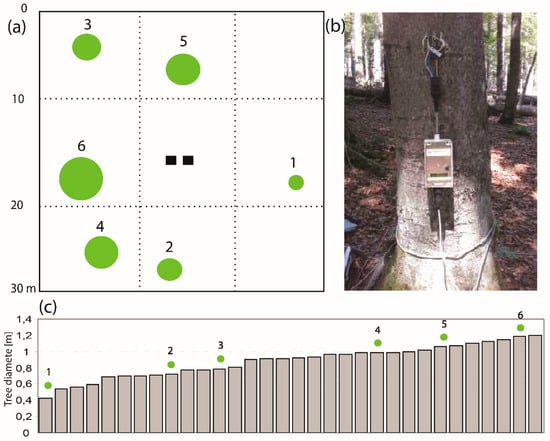
Figure 3.
(a) Scheme of the tree distribution for sap flow measurement at the 30 × 30-m experimental plot. Note: the size of the green dot represents the size of the tree trunk, two black squares are the rough location of two tensiometers. (b) Photo of one installed EMS 81 sap flow device at 1 m above the ground in Tree No. 1. (c) Tree trunk diameter (in m) distribution at 1-m height within 32 beech trees over the experimental plot. Note: the green dots mark the measured trees.
In our study plot, the square area (30 × 30 m) of 900 m2 consisted of 32 beech trees with the mean age of 55 years and the mean trunk diameter of 0.9 m (at the height of 1 m) (Figure 3a,c). Six trees were selected based on the representative diameter at breast height (DBH), trunk curvature, etc., and sap flow equipment was installed on these six selected trees with different ages and trunk diameters (see a photo in Figure 3b).
Sap flow was measured using the stem tissue heat balance method (THB) with constant heating power, as described by Čermák, et al. [39]. The data were recorded on a data logger every 30 min, at the height of 1.0 m above ground (Figure 3b), using EMS 81 sap flow equipment (EMS Brno, CZ). Each EMS 81 equipment includes 4 heat sensors (see the equipment in Figure 3b). The THB method quantifies the amount of heat transported by water flow across a predefined area within the xylem conduit, as a percentage of the total heat supplied. In this study, the sap flow rate Q (kg s−1) is calculated by
where P(W) is power of heat input, cw (J kg−1K−1) is the specific heat of water, ø (W K−1) is the coefficient of heat loss from the measuring point, ▽T (K) is the temperature gradient at the measuring point, and d (cm) is the effective width of the measuring point (d = 5.5 cm in this study). The first term in the right hand side of Equation (2) quantifies the heat conducted by sap flow, while the second term in right hand side of Equation (2) represents the heat loss from the sensor [39].
The scaling up of sap flow from six sample trees to the stand level was based on the DBH of the sample trees and diameter distribution of the trees in the forest stand according to the methodology developed by Čermák et al. [39]. The specific method of how we worked with a distribution of trunk DBH per area is:
- Classified groups of the trunk DBH and calculated canopy conductance from sap flow for each group (step 10 cm);
- Calculated ratio of the number of trees per DBH group;
- Recalculated canopy conductance from groups to tree DBH.
In this study plot, the beech stand covered approximately 0.4 km2. The leaf area index (LAI) was measured by the hemispherical photos. The photos were taken by a Nikon COOLPIX 995 camera (Nikon, Japan) with Nikon Fisheye lens Converter FC-E8 (Nikon, Japan) 0.21x in a square (30 × 30 m) in a step of 10 m. Thus, 16 pictures were taken and analysed for leaf area index in Gap Light Analyser (GLA) software [40].
2.3. Canopy Stomatal Conductance Calculation
In vegetated areas, the transpiration rate is dictated by the parameter of stomatal conductance, (m s−1). If the transpiration rate (e.g., from sap flow measurement) and climatic measurements are available, the stomatal conductance can then be inversely estimated by rearranging the Penman–Monteith-type equation:
where (mm s−1) is the stand transpiration calculated from the sap flow measurements; (kPa K−1) is the gradient of the saturation vapour pressure-temperature curve; (kPa) is the vapour pressure of evaporative surface; (kPa) is the vapour pressure of atmospheric air; (kPa) is the vapour pressure deficit (D); (kg m−3) and (MJ kg−1 K−1) are the density and specific heat capacity of the atmospheric air; (kPa K−1) is the psychrometric constant; (m s−1) is stomatal conductance, and (m s−1) is the aerodynamic conductance that is a function of wind speed at the canopy height, (m s−1), and (W m−2) is the net radiation received by canopy layer:
where (W m−2) is the net radiation of the land surface, and is the extinction coefficient of the vegetation for net radiation, and the typical value for forest is 0.5 [41]. Using this equation here, we simply assume the net radiation received by canopy layer is a constant fraction of the net radiation of the land surface, which means that the effect of leaf angle distribution on shortwave irradiance was neglected.
The aerodynamic resistance (= 1/) is calculated by:
where (=0.5) is the shielding factor; is the characteristic leaf width with a typical value of 0.2 m for a broadleaf forest [42]; is the eddy diffusivity decay constant that may be set to 4.25 for forest area [43]; and (-) is the leaf area index.
The canopy conductance of a beech forest was examined at hourly time steps and daily steps on a 30 × 30-m canopy with a LAI of 3.2 in three months of 2015. Sap flow measurement was conducted in a plot over the middle of summer and the beginning of autumn (day of year DOY 203–302, i.e., 23 July–30 October) in the year of 2015.
The stomatal conductance is controlled by stomatal aperture in response to the availability of energy, carbon, and water in soil [14,17]. Considering the impact of multiple environmental factors on stomatal conductance, this study adopted the Jarvis–Stewart model [43,44], which consists of multiplicative nonlinear functions of environmental variables [19,20,43,45]:
where is the leaf area index ( = 2.2 measured in this study), and (m s−1) denotes the theoretical maximum under the optimal water, nutrient, and climatic conditions. The functions are a set of scaling terms that reduced a maximum value of canopy conductance () in response to changes in net radiation (Rs), vapour pressure deficit (D), temperature (T), and soil water content (). The values of functions range between 0 and 1. Therefore, any changes in the values of Rs, D, T, and will proportionally modify the parameters to give an estimation of the controlling transpiration rate. The multiplicative stress functions are taken from previous studies [42,44,46,47,48].
3. Results
3.1. Meteorological Parameters, Soil Moisture and Sap Flow
The mean maximum daily solar radiation for both the vegetation period (DOY203–272) and leaf-fallen period (DOY 273–302) was similar to the 5-year (2013–2017) average value (see Table 1). In the studied period, the maximum daily solar radiation peaked to more than 1100 W m−2 when it was sunny at noon (during the summer), while during the rainy or cloudy days, the daily maximum solar radiation bottomed out to lower than 200 W m−2.

Table 1.
Meteorological conditions in the study area.
Generally, there was a clear decreasing trend of the air temperature over the period. During the vegetation period before DOY 272) (Figure 4), the daily mean air temperature was approximately 13.3 ℃, ranging between 6 and 31.3 ℃, which was still comparable with the 5-year average of 15.7 ℃ for this period. Temperature started to drop significantly after DOY 280, along with the reduced daily maximum solar radiation. During the period of DOY 273–302, the daily mean air temperature was approximately 4.6 ℃, ranging between −6 and 18.7 ℃. A lower temperature during the days of our measurements was quite common, while morning values got usually below zero from August. The wind speed in the study area over the study period had no clear pattern and the trend fluctuated with an average of 1.2 m s−1, which was similar to the past 5-year average of 1.5 m s−1 for this period. The study area was located in a relatively humid area [26,27], which was evident during the study period in 2015 (see both Figure 4d and Figure 5b). The measured daily mean relative humidity remained at over 77% for two periods. The daily variability of the relative humidity was larger during autumn than in summer.
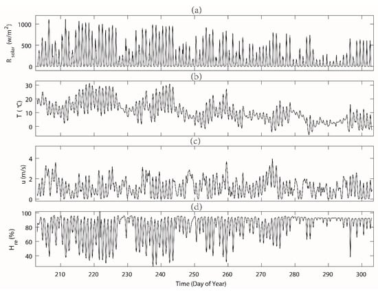
Figure 4.
The measured micro-meteorological variables at hourly intervals during the day of year (DOY) 203–302 in station Rokytka (ROK). The variables including (a) Rs—incoming solar radiation, (b) T—air temperature, (c) u—wind speed, and (d) Hre—relative humidity. See the exact values in Table 1.
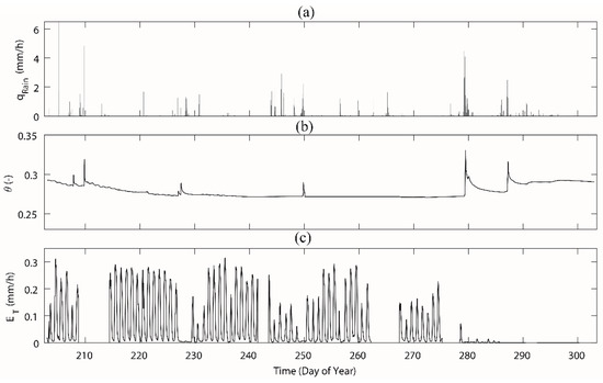
Figure 5.
The measurements of (a) rainfall, (b) soil moisture, and (c) stand sap flow in the study area Rokytka (ROK) during the day of year 203–302. Abbreviations: qrain—rainfall, —averaged soil moisture based on measured soil moisture from a depth of 20 cm and 60 cm, ET—calculated transpiration based on measured sap flow from six beech trees. A data gap of transpiration from DOY 209–213 (i.e., 29 July–2 August) was due to a lack of battery power in the sensors.
Rainfall in the study area featured a temperate mountainous pattern and the total rainfall was 224.6 mm during the measured period (Figure 5), which was slightly lower than the 5-year average of 310 mm. DOY 230–243 (Figure 5) experienced a rainless period. The consecutive rain events happened on DOY 278–281, and soil moisture increased significantly. Over the study period, the mean soil moisture content at 60 cm depth was 0.22, while it was 0.36 at 20 cm depth (Figure 5 shows the averaged values), which was much smaller than their 5-year averages. The 5-year average of soil moisture is 0.62 at 20 cm depth and 0.27 at 60 cm depth. During the study period, after consecutive rain events, the soil moisture content increased up to 0.35 (0.30 at 60 cm depth and 0.40 at 20 cm depth; Figure 5), which was similar to the 5-year average for the deep soil but the upper soil was still dryer than the 5-year average.
The diurnal pattern of the measured sap flow in the six trees were similar but with significant differences in the exact maximum values due to the size of the trees (Figure S1). Therefore, transpiration was measured with the sap flow sensors and scaled to the study plot by considering all the existing trees in the plot. The calculated transpiration reached its maximum values approximately 0.32 mm/h during sunny days. In those days, the daily variability was higher than in the rainy days and in non-vegetation periods (Figure 5). Transpiration was dramatically decreased when the leaves started to fall down from DOY 270 and by the DOY 280, the leaves had all fallen and transpiration dropped to nearly zero.
The transition from the vegetative period to the deciduous period (when sap flow measurement reached 0) happened slightly differently in each tree over 8 days between DOY 277 and DOY 284. Two factors could be connected to the leaf fall, the long-term rain from DOY 279 to DOY 280, with a total rainfall of 39 mm, and the air temperature as freezing nights occurred more often after October (i.e., DOY 273).
3.2. Diurnal Behaviours of Stomatal Conductance and Responses of Canopy Conductance
The diurnal variation of stomatal conductance had common patterns for different vegetation periods (Figure 6). The lower value in the morning and the afternoon and a higher value at midday depended on the diurnal pattern of solar radiation and relative humidity (given in Figure 7). The lower stomatal conductance at midday (13.00) than before and after approximately 13.00, Figure 6c for instance, can be attributed to the higher vapour deficit. In some extreme cases, the hydraulic potential on leaf surface is much higher than the potential at root layer due to, for instance, low humidity or high wind speed. Trees cannot sustain such a pressure and start to decrease the transpiration process. In autumn periods (Figure 6d), the inversely calculated stomatal conductance values approach smaller values. The physiological behaviour of trees has a significant transition because the trees lose leaves every year with the change of the seasons. The transition in stomatal behaviour during the deciduous period has a significant impact on transpiration. However, the estimation of stomatal conductance did not account the transition from the vegetative period to the deciduous period. The canopy conductance was responding to the net radiation, vapour pressure deficit, and soil moisture (Figure 7). A typical parameter set for the deciduous broadleaf forests in a lookup table [42] of the parameterization of the Jarvis–Stewart model provided a boundary reference for each stress parameter (Table 2). The scatter in the plot of F1–Rs (Figure 7a) was rather large, and we cannot find a clear relationship between solar radiation and normalized stomatal conductance. The F1 function (line in Figure 7a) showed that the gc responses to Rs are almost identical, showing that Rs increases along with gc asymptotically from zero to a maximum. The functional forms (line in Figure 7b,c) of F2 (D) and F3 (T) are described well to the scatters described by the measured data, describing the response of vapour pressure deficit and temperature to the canopy conductance. The impact of soil moisture stress on transpiration (stress function F4) is very small, and the dots fall into a small range (Figure 7d), because the soil moisture in the study area remains at a relatively high level (over 0.27). The function covers the full range of the soil moisture response, which did not occur in the study period.
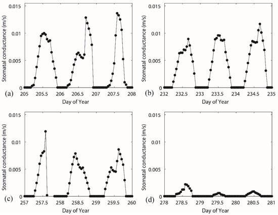
Figure 6.
Canopy conductance inversely calculated from the Penman–Monteith equation over four selected periods, including (a) DOY 205–DOY208, (b) DOY 232–DOY 235, (c) DOY 257– DOY 260, and (d) DOY 278–DOY 281, which were covering from the vegetative period to the deciduous period.
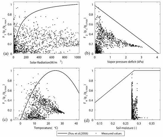
Figure 7.
Response of stress functions in canopy conductance to (a) net radiation (Rs), (b) vapor pressure deficit (D), (c) temperature (T), and (d) soil moisture (). The line for each sub-figure was using the parameter given by Zhou et al. [42], see Table 2.
Table 2.
The stress functions of canopy conductance to net radiation (Rs), vapor pressure deficit (D), temperature (T), and soil moisture () with calibrated parameters and Zhou et al. [42]’s parameters (see the blue line and line given in Figure 6).
4. Discussion
Stomatal behaviour varies among tree species due to different parametrizations of gc [24]. Many physiological models for describing the response of stomatal conductance, gc, to environmental stress have been proposed, such as the Jarvis–Stewart model [43], and the Ball–Berry model [49]. For general vegetation types (e.g., broadleaf forests, needle leaf forests, shrub lands, croplands, grasslands, etc.), the parametrizations of gc were available in a lookup table [5,21,24,42,50,51]. These standard parametrizations have been used to estimate the moisture flux from land surface at a catchment scale or even at a global scale [51,52,53]. However, stomatal behaviour commonly shows distinct properties even within a certain tree species [54,55]. For a certain study site, general parametrization of one type of vegetation species may not be fully represented [42]. In particular, for an area that has experienced severe changes in the distribution of tree species under climate change and insect-induced forest disturbance, it is necessary to inversely estimate gc from sap flow measurement for special tree species.
This study explored the response of leaf stomata to multiple environmental factors of solar radiation, vapour pressure deficit, air temperature and soil moisture, and the key finding from this study was that the measured stomatal behaviour (see in Figure 7) showed a large discrepancy compared with the typical parameter set of the deciduous forest which was often used. We found that the leaf stomatal conductance inferred from sap flow data did not show clear responses to solar radiation and soil moisture, and even show a less clear response to the air temperature. Stomatal conductance calculated from sap flow show lower values than it can be estimated from Zhou´s parameters [42]. A lower stomatal conductance at midday can be explained by a limitation of photosynthesis due to the stomatal closure to prevent the water loss from intensive solar radiation and high temperatures. In general, energy supply theoretically limits evaporation during low radiation periods (when Rs <200 W m−2), in contrast with high radiation periods (when Rs >200 W m−2). However, the principle in forest areas and high latitude regions may be not the same. Köstner [56] also found that on the daily basis, stomatal conductance and Rs for beech forest in Germany showed a near linear relation and available energy was not a limiting factor for transpiration considering only 40~75% of net radiation was used for beech transpiration.
The results of stomatal response showed that the soil moisture did not constrain transpiration considering its value was relatively high during the study period. Williams, et al. [57] also found soil moisture was not a frequent stress factor in many forest stands including beech due to relatively abundant rainfall, which was consistent with the previous studies conducted in Central Europe that [56,58,59]. The soil moisture content and sap flow of trees are less comparable in beech stand than in spruce stands. The reason for this could be the high rooting depth of beech tree stand. Spruces create shallow rooting zones (<50 cm). Therefore, they suck water from upper soil layers and can be comparable with the evaporation process from soil surface. On the other hand, beech stands receive non-negligible quantity of water from deeper horizons (from regolith) and therefore they dry less at soil surface or upper soil horizons. This could be a reason for why gc does not perfectly fit to soil moisture. Notwithstanding that our measurements were determined during a period with less rainfall, the root system of a beech can reach a depth of several meters [60,61], sucking water from lower layers. This study was focused in a soil profile up to the depth of 1 m which is drained generally by fine shallow root systems [60]. On the other hand, we assumed lower evaporation from soil surface could be shaded by trees, covered with fallen leaves and dead wood. In addition, our data did not show any shifts in soil tension described by Or, et al. [62].
From the previous study concerning subsurface flow mechanisms in this study site [37], the dominant subsurface flow is biomat flow (i.e., shallow subsurface flow) and deep percolation. Biomat flow is mostly caused by stormflow events [63], and deep percolation is connected with slow infiltration and long-term water storage (e.g., from snow melt). It is evident that each tree species (spruce x beech) is connected with different sources of water, and respectively different flow mechanisms in soil. If spruce stands were replaced by beech stands, it would have an impact on water storage in soil or regolith. It is possible to consider that beech stands together with decreasing snow cover can contribute to a change in runoff formation, respectively, to emptying deep water aquifers.
The response of gc to vapour pressure deficit (VPD) demonstrated clear patterns. The increasing VPD shows similar trend with other studies [42,64] that have found an exponential response. However, a linear relationship was also often adopted in many prior studies to describe the constrain of VPD on gc [42]. The response of gc to air temperature may be described with a quadratic function or a bell-shape function, and our study showed a slight scattered relation. Kučera, et al. [17] mentioned that the estimated time lags between the sap flow and climate variables were 60 min for Rg and 30 min for D, and such hysteresis loops that we did not consider. This issue will influence the accuracy of the simulated timing.
5. Conclusions
This study focused on estimating the stomatal conductance using the measured sap flow at a newly formed beech stand, Šumava Mts. (the Czech Republic). Due to a bark beetle outbreak in the area, mixed forest stands (spruce and beech) have transformed into beech stands. From the differences of the rooting depth of each kind of tree, an impact on long-term water regime is expected. Trees can change soil moisture distribution or water storage in aquifers by transpiration. Therefore, our study was focused on the stomatal conductance of newly formed beech stands. The measured sap flow data were used to inversely estimate the stomatal conductance through the Penman–Monteith equation. The stomatal conductance reached the highest value at midday but, on some days, there was a sudden drop at midday. A drop of stomatal conductance at midday can be explained by a limitation of photosynthesis due to the stomatal closure to prevent the water loss from the most intensive solar radiation and higher temperature. We also found that the calculated stomatal conductance decreased dramatically in the deciduous period, as the estimation based on the Penman–Monteith equation did not account for the vegetation transition from the vegetative period to the deciduous period.
The parameterization of the Jarvis–Stewart model was used to describe the response of stomatal conductance under the varying environmental conditions of net radiation, vapour pressure deficit, temperature, and soil water content. The stomatal conductance showed a good relationship (connection) with vapour deficit but low correlation with soil moisture. The temperature showed a certain relation but not one as strong as the vapour deficit, which might be due to the smaller range during our study period that went without experiencing a wide spectrum of temperature. The soil moisture did not constrain transpiration considering its value is relatively high during the study period. Therefore, in the study area, vapour deficit and temperature are two key factors impacting the transpiration processes. The most important finding is that the parametrization of stress functions based on the typical deciduous forest does not perfectly represent the measured stomatal response of newly formed beech stands. Therefore, the sap flow results can provide valuable data to better understanding the evapotranspiration process in newly formed beech stands after the bark beetle outbreak in Central Europe.
Supplementary Materials
The following are available online at https://www.mdpi.com/2076-3263/9/5/243/s1, Figure S1: The diurnal pattern of the measured sap flow in 6 trees (the sizes of the six trees in corresponding numbers are given in Figure 3a.) at two selected days – DOY 205 and DOY 207.
Author Contributions
Conceptualization, Y.S.; Data curation, L.V. and Y.S.; Formal analysis, Y.S. and W.S.; Funding acquisition, W.S. and J.L.; Investigation, Y.S. and L.V.; Methodology, Y.S. and W.S.; Project administration, L.V. and J.L.; Resources, J.L.; Software, Y.S. and W.S.; Supervision, J.L.; Validation, Y.S.; Visualization, Y.S. and W.S.; Writing—original draft, Y.S.; Writing—review and editing, Y.S.
Funding
This study was financially supported by Czech Science Foundation project 19-05011S, EU COST Action ES1306, project LD 15130 "Impact of landscape disturbance on stream and basin connectivity", and the National Natural Science Foundation of China (Grant Nos. 41807286), the China Postdoctoral Science Foundation (Grant Nos. 2017M621783, 2018T110527), the International Postdoctoral Exchange Fellowship Program by China Postdoctoral Council (Year 2017), and the Startup Foundation for Introducing Talent of NUIST (No.2017r045).
Acknowledgments
We thank Josef Urban (Menedl University in Brno) for assisting us in installing the sap flow devices and processing the raw data and EMS company for providing the sap flow devices.
Conflicts of Interest
The authors declare no conflict of interest. The funders had no role in the design of the study; in the collection, analyses, or interpretation of data; in the writing of the manuscript, or in the decision to publish the results.
References
- Moreira, M.; Sternberg, L.; Martinelli, L.; Victoria, R.; Barbosa, E.; Bonates, L.; Nepstad, D. Contribution of transpiration to forest ambient vapour based on isotopic measurements. Chang. Boil. 1997, 3, 439–450. [Google Scholar] [CrossRef]
- Ewers, B.; Mackay, D.; Gower, S.; Ahl, D.; Burrows, S.; Samanta, S. Tree species effects on stand transpiration in northern Wisconsin. Water Resour. Res. 2002, 38, 8-1–8-11. [Google Scholar] [CrossRef]
- Schlesinger, W.H.; Jasechko, S. Transpiration in the global water cycle. Agric. Meteorol. 2014, 189, 115–117. [Google Scholar] [CrossRef]
- Buckley, T.N.; Mott, K.A. Modelling stomatal conductance in response to environmental factors. Plant Cell Environ. 2013, 36, 1691–1699. [Google Scholar] [CrossRef] [PubMed]
- Wehr, R.; Commane, R.; Munger, J.W.; McManus, J.B.; Nelson, D.D.; Zahniser, M.S.; Saleska, S.R.; Wofsy, S.C. Dynamics of canopy stomatal conductance, transpiration, and evaporation in a temperate deciduous forest, validated by carbonyl sulfide uptake. Biogeosciences 2017, 14, 389–401. [Google Scholar] [CrossRef]
- Rao, P.; Agaewal, S.K. Diurnal variation in leaf water potential, stomatal conductance, and irradiance of winter crop under different moisture levels. Boil. Plant. 1984, 26, 1–4. [Google Scholar] [CrossRef]
- Lin, Y.-S.; Medlyn, B.E.; Duursma, R.A.; Prentice, I.C.; Wang, H.; Baig, S.; Eamus, D.; De Dios, V.R.; Mitchell, P.; Ellsworth, D.S.; et al. Optimal stomatal behaviour around the world. Nat. Clim. Chang. 2015, 5, 459–464. [Google Scholar] [CrossRef]
- Monteith, J. Evaporation and environment. Symp. Soc. Exp. Biol. 1965, 4, 205–234. [Google Scholar]
- Allen, R.G.; Pereira, L.S.; Raes, D.; Smith, M. Crop Evapotranspiration-Guidelines for Computing Crop Water Requirements-Fao Irrigation and Drainage Paper 56; Food and Agriculture Organization of the United Nations (FAO): Rome, Italy, 1998; Volume 300, p. D05109. [Google Scholar]
- Monteith, J. Evaporation and surface temperature. Q. J. Meteorol. Soc. 1981, 107, 1–27. [Google Scholar] [CrossRef]
- Iritz, Z.; Tourula, T.; Lindroth, A.; Heikinheimo, M. Simulation of willow short-rotation forest evaporation using a modified Shuttleworth-Wallace approach. Hydrol. Process. 2001, 15, 97–113. [Google Scholar] [CrossRef]
- Whitley, R.; Medlyn, B.; Zeppel, M.; Macinnis-Ng, C.; Eamus, D.; Macinnis-Ng, C. Comparing the Penman–Monteith equation and a modified Jarvis–Stewart model with an artificial neural network to estimate stand-scale transpiration and canopy conductance. J. Hydrol. 2009, 373, 256–266. [Google Scholar] [CrossRef]
- Guan, H.; Wilson, J.L. A hybrid dual-source model for potential evaporation and transpiration partitioning. J. Hydrol. 2009, 377, 405–416. [Google Scholar] [CrossRef]
- Damour, G.; Simonneau, T.; Cochard, H.; Urban, L. An overview of models of stomatal conductance at the leaf level. Plant Cell 2010, 33, 1419–1438. [Google Scholar] [CrossRef]
- Hernandez-Santana, V.; Fernández, J.; Rodriguez-Dominguez, C.; Romero, R.; Diaz-Espejo, A. The dynamics of radial sap flux density reflects changes in stomatal conductance in response to soil and air water deficit. Agric. Meteorol. 2016, 218, 92–101. [Google Scholar] [CrossRef]
- Čermák, J.; Cienciala, E.; Kucera, J.; Lindroth, A.; Bednárová, E. Individual variation of sap-flow rate in large pine and spruce trees and stand transpiration: A pilot study at the central NOPEX site. J. Hydrol. 1995, 168, 17–27. [Google Scholar] [CrossRef]
- Kučera, J.; Brito, P.; Jiménez, M.S.; Urban, J. Direct Penman–Monteith parameterization for estimating stomatal conductance and modeling sap flow. Trees 2017, 31, 873–885. [Google Scholar] [CrossRef]
- Köstner, B.M.M.; Schulze, E.-D.; Kelliher, F.M.; Hollinger, D.Y.; Byers, J.N.; Hunt, J.E.; McSeveny, T.M.; Meserth, R.; Weir, P.L. Transpiration and canopy conductance in a pristine broad-leaved forest of Nothofagus: An analysis of xylem sap flow and eddy correlation measurements. Oecologia 1992, 91, 350–359. [Google Scholar] [CrossRef] [PubMed]
- Naithani, K.J.; Ewers, B.E.; Pendall, E. Sap flux-scaled transpiration and stomatal conductance response to soil and atmospheric drought in a semi-arid sagebrush ecosystem. J. Hydrol. 2012, 464, 176–185. [Google Scholar] [CrossRef]
- Wang, H.; Guan, H.; Deng, Z.; Simmons, C.T. Optimization of canopy conductance models from concurrent measurements of sap flow and stem water potential on Drooping Sheoak in South Australia. Water Resour. 2014, 50, 6154–6167. [Google Scholar] [CrossRef]
- Granier, A.; Biron, P.; Lemoine, D. Water balance, transpiration and canopy conductance in two beech stands. Agric. Meteorol. 2000, 100, 291–308. [Google Scholar] [CrossRef]
- Roberts, J. The influence of physical and physiological characteristics of vegetation on their hydrological response. Hydrol. Process. 2000, 14, 2885–2901. [Google Scholar] [CrossRef]
- Vertessy, R.A.; Benyon, R.G.; O’Sullivan, S.K.; Gribben, P.R. Relationships between stem diameter, sapwood area, leaf area and transpiration in a young mountain ash forest. Tree Physiol. 1995, 15, 559–567. [Google Scholar] [CrossRef]
- Ewers, B.E.; Gower, S.T.; Wang, C.K.; Bond-Lamberty, B.; Bond-Lamberty, B.; Bond-Lamberty, B. Effects of stand age and tree species on canopy transpiration and average stomatal conductance of boreal forests. Plant Cell 2005, 28, 660–678. [Google Scholar] [CrossRef]
- Bernsteinová, J.; Bässler, C.; Zimmermann, L.; Langhammer, J.; Beudert, B. Changes in runoff in two neighbouring catchments in the Bohemian Forest related to climate and land cover changes. J. Hydrol. Hydromech. 2015, 63, 342–352. [Google Scholar] [CrossRef]
- Langhammer, J.; Su, Y.; Bernsteinová, J. Runoff Response to Climate Warming and Forest Disturbance in a Mid-Mountain Basin. Water 2015, 7, 3320–3342. [Google Scholar] [CrossRef]
- Su, Y.; Langhammer, J.; Jarsjö, J. Geochemical responses of forested catchments to bark beetle infestation: Evidence from high frequency in-stream electrical conductivity monitoring. J. Hydrol. 2017, 550, 635–649. [Google Scholar] [CrossRef]
- Oulehle, F.; Chuman, T.; Majer, V.; Hruška, J. Chemical recovery of acidified Bohemian lakes between 1984 and 2012: The role of acid deposition and bark beetle induced forest disturbance. Biogeochemistry 2013, 116, 83–101. [Google Scholar] [CrossRef]
- Tesař, M.; Šír, M.; Dvořák, I.J.; Lichner, Ľ. Influence of vegetative cover changes on the soil water regime in headwater regions in the Czech Republic. IHP/HWRP-Berichte 2004, 2, 57–72. [Google Scholar]
- Hais, M.; Kučera, T. Surface temperature change of spruce forest as a result of bark beetle attack: Remote sensing and GIS approach. Eur. J. 2008, 127, 327–336. [Google Scholar] [CrossRef]
- Wild, J.; Kopecký, M.; Svoboda, M.; Zenáhlíková, J.; Edwards-Jonášová, M.; Herben, T. Spatial patterns with memory: Tree regeneration after stand-replacing disturbance in Picea abies mountain forests. J. Veg. Sci. 2014, 25, 1327–1340. [Google Scholar] [CrossRef]
- Schipka, F.; Heimann, J.; Leuschner, C. Regional variation in canopy transpiration of Central European beech forests. Oecologia 2005, 143, 260–270. [Google Scholar] [CrossRef] [PubMed]
- Schume, H.; Hager, H.; Jost, G. Water and energy exchange above a mixed European Beech—Norway Spruce forest canopy: A comparison of eddy covariance against soil water depletion measurement. Theor. Appl. Climatol. 2005, 81, 87–100. [Google Scholar] [CrossRef]
- Střelcová, K.; Minďáš, J.; Škvarenina, J. Influence of tree transpiration on mass water balance of mixed mountain forests of the West Carpathians. Biologia 2006, 61, S305–S310. [Google Scholar] [CrossRef]
- Heil, K. Wasserhaushalt und Stoffumsatz in Fichten- (Picea abies (L.) Karst.) und Bucheno¨kosystemen (Fagus Sylvatica L.) der ho¨Heren Lagen des Bayerischen Waldes. Ph.D. Thesis, University of Munich, München, Germany, 1996. [Google Scholar]
- Čada, V.; Svoboda, M.; Janda, P. Dendrochronological reconstruction of the disturbance history and past development of the mountain Norway spruce in the Bohemian Forest, central Europe. Ecol. Manag. 2013, 295, 59–68. [Google Scholar] [CrossRef]
- Vlček, L.; Falátková, K.; Schneider, P. Identification of runoff formation with two dyes in a mid-latitude mountain headwater. Hydrol. Earth Sci. 2017, 21, 3025–3040. [Google Scholar]
- Van Genuchten, M.T.; Leij, F.; Yates, S. The Retc Code for Quantifying the Hydraulic Functions of Unsaturated Soils; US Salinity Laboratory: Riverside, CA, USA, 1991. [Google Scholar]
- Čermák, J.; Kučera, J.; Nadezhdina, N. Sap flow measurements with some thermodynamic methods, flow integration within trees and scaling up from sample trees to entire forest stands. Trees 2004, 18, 529–546. [Google Scholar] [CrossRef]
- Frazer, G.W.; Trofymow, J.A.; Lertzman, K.P. A Method for Estimating Canopy Openness, Effective Leaf Area Index, and Photosynthetically Active Photon Flux Density Using Hemispherical Photography and Computerized Image Analysis Techniques; Information Report BC-X-373; Pacific Forestry Centre, Natural Resources Canada: Victoria, BC, Canada, 1997; p. 73. [Google Scholar]
- Monteith, J.; Unsworth, M. Principles of Environmental Physics: Plants, Animals, and the Atmosphere, 4th ed.; Academic Press: Cambridge, MA, USA, 2013. [Google Scholar]
- Zhou, M.; Ishidaira, H.; Hapuarachchi, H.; Magome, J.; Kiem, A.; Takeuchi, K.; Kiem, A. Estimating potential evapotranspiration using Shuttleworth–Wallace model and NOAA-AVHRR NDVI data to feed a distributed hydrological model over the Mekong River basin. J. Hydrol. 2006, 327, 151–173. [Google Scholar] [CrossRef]
- Jarvis, P.G. The Interpretation of the Variations in Leaf Water Potential and Stomatal Conductance Found in Canopies in the Field. Philos. Trans. Soc. B Biol. Sci. 1976, 273, 593–610. [Google Scholar] [CrossRef]
- Stewart, J. Modelling surface conductance of pine forest. Agric. Meteorol. 1988, 43, 19–35. [Google Scholar] [CrossRef]
- Zhang, B.; Liu, Y.; Xu, D.; Cai, J.; Li, F. Evapotranspiraton estimation based on scaling up from leaf stomatal conductance to canopy conductance. Agric. Meteorol. 2011, 151, 1086–1095. [Google Scholar] [CrossRef]
- Granier, A.; Ceschia, E.; Damesin, C.; Lebaube, S.; Le Dantec, V.; Lemoine, D.; Lucot, E.; Pontailler, J.Y.; Dufrêne, E.; Epron, D.; et al. The carbon balance of a young Beech forest. Funct. Ecol. 2000, 14, 312–325. [Google Scholar] [CrossRef]
- Magnani, F.; Leonardi, S.; Tognetti, R.; Grace, J.; Borghetti, M. Modelling the surface conductance of a broad-leaf canopy: Effects of partial decoupling from the atmosphere. Plant Cell 1998, 21, 867–879. [Google Scholar] [CrossRef]
- Zhang, L.; Brook, J.R.; Vet, R. A revised parameterization for gaseous dry deposition in air-quality models. Atmos. Chem. Phys. Discuss. 2003, 3, 2067–2082. [Google Scholar] [CrossRef]
- Ball, J.T.; Woodrow, I.E.; Berry, J.A. A Model Predicting Stomatal Conductance and its Contribution to the Control of Photosynthesis under Different Environmental Conditions. In Progress in Photosynthesis Research; Springer Nature: Basingstoke, UK, 1987; pp. 221–224. [Google Scholar]
- Gerosa, G.; Mereu, S.; Finco, A.; Marzuoli, R. Stomatal Conductance Modeling to Estimate the Evapotranspiration of Natural and Agricultural Ecosystems. In Evapotranspiration—Remote Sensing and Modeling; Irmak, A., Ed.; Inech: Rijeka, Croatia, 2012; pp. 403–420. [Google Scholar]
- Ge, Z.-M.; Zhou, X.; Kellomäki, S.; Peltola, H.; Wang, K.-Y. Climate, canopy conductance and leaf area development controls on evapotranspiration in a boreal coniferous forest over a 10-year period: A united model assessment. Ecol. Model. 2011, 222, 1626–1638. [Google Scholar] [CrossRef]
- Viterbo, P.; Beljaars, A.C.M. An Improved Land Surface Parameterization Scheme in the ECMWF Model and Its Validation. J. Clim. 1995, 8, 2716–2748. [Google Scholar] [CrossRef]
- Tiedtke, M. ECMWF Model Parameterisation of Sub-Grid Scale Processes; European Centre for Medium Range Weather Forecast: Reading, UK, 1979. [Google Scholar]
- Tateishi, M.; Kumagai, T.; Suyama, Y.; Hiura, T. Differences in transpiration characteristics of Japanese beech trees, Fagus crenata, in Japan. Tree Physiol. 2010, 30, 748–760. [Google Scholar] [CrossRef][Green Version]
- Shao, W.; Su, Y.; Langhammer, J. Simulations of coupled non-isothermal soil moisture transport and evaporation fluxes in a forest area. J. Hydrol. Hydromech. 2017, 65, 410–425. [Google Scholar] [CrossRef][Green Version]
- Köstner, B. Evaporation and transpiration from forests in Central Europe—Relevance of patch-level studies for spatial scaling. Theor. Appl. Clim. 2001, 76, 69–82. [Google Scholar]
- Williams, M.; Malhi, Y.; Nobre, A.D.; Rastetter, E.; Pereira, M.G.P. Seasonal variation in net carbon exchange and evapotranspiration in a Brazilian rain forest: A modelling analysis. Plant Cell Environ. 1998, 21, 953–968. [Google Scholar] [CrossRef]
- Herbst, M.; Eschenbach, C.; Kappen, L. Water use in neighbouring stands of beech (Fagus sylvatica L.) and black alder (Alnus glutinosa (L.) Gaertn.). Ann. For. Sci. 1999, 56, 107–120. [Google Scholar] [CrossRef]
- Körner, C. Humidity responses in forest trees: Precautions in thermal scanning surveys. Theor. Appl. Clim. 1985, 36, 83–98. [Google Scholar] [CrossRef]
- Harley, J.L. A Study of the Root System of the Beech in Woodland Soils, with Especial Reference to Mycorrhizal Infection. J. Ecol. 1940, 28, 107. [Google Scholar] [CrossRef]
- David, T.S.; Pinto, C.A.; Nadezhdina, N.; Kurz-Besson, C.; Henriques, M.O.; Quilhó, T.; Čermák, J.; Chaves, M.M.; Pereira, J.S.; David, J.S. Root functioning, tree water use and hydraulic redistribution in Quercus suber trees: A modeling approach based on root sap flow. Ecol. Manag. 2013, 307, 136–146. [Google Scholar] [CrossRef]
- Or, D.; Lehmann, P.; Shahraeeni, E.; Shokri, N. Advances in Soil Evaporation Physics—A Review. Vadose Zone J. 2013, 12, 12. [Google Scholar] [CrossRef]
- Gerke, K.M.; Sidle, R.C.; Mallants, D. Preferential flow mechanisms identified from staining experiments in forested hillslopes. Hydrol. Process. 2015, 29, 4562–4578. [Google Scholar] [CrossRef]
- Granier, A.; Loustau, D. Measuring and modelling the transpiration of a maritime pine canopy from sap-flow data. Agric. Meteorol. 1994, 71, 61–81. [Google Scholar] [CrossRef]


© 2019 by the authors. Licensee MDPI, Basel, Switzerland. This article is an open access article distributed under the terms and conditions of the Creative Commons Attribution (CC BY) license (http://creativecommons.org/licenses/by/4.0/).