Abstract
The Pechora Sea is optimally located for studying the coalescence of a glacial and periglacial continental shelf zone in the high Arctic. Here, we present data acquired during cruises of the RV Akademik Nikolaj Strakhov in 2018–2021, revealing the distribution of submarine glacial landforms in the central part of the Pechora shelf area. Based on moraines and the distribution of glacial lineations, the extent of the ice sheet during the Last Glacial Maximum (LGM) is proposed. The crests of the moraine ridges and the slopes of their sides express a variation in morphology, and the ridges combine into irregular complexes. The moraines are primarily composed of coarse cobble-sized material with an addition of coarse sand and other sedimentary fractions. The mapped glacial landforms clearly indicate that an ice sheet extended over the area, while the Pechora basin, at the same time, was comprised of lowland characterized by a cryogenic subaerial landscape. Based on the result from this study, the extent and ice-flow pattern of the Barents-Kara Ice Sheet during the LGM were determined.
1. Introduction
The most prominent and widespread submarine landforms on the Arctic continental shelf were formed by the Quaternary Ice Sheets [1]. The identification of these glacial landforms and the determination of the processes forming them are facilitated by high-quality bathymetric mapping and sub-bottom profiling. Many relief-forming processes on the seafloor, glacial or non-glacial, do not take place steadily but change over time. Thus, it is often possible to distinguish seafloor features formed by modern ongoing processes from those formed by paleo-processes. The seafloor morphology of the present Arctic Ocean continental shelf, with the exception of areas that were not covered by ice sheets, was, to a large extent, formed during the Last Glacial Maximum (LGM) [2,3].
The south-eastern part of the Barents Sea between the Kolguev and Vaygach islands is commonly referred to as the Pechora Sea (Figure 1). The morphology and structure of the seabed differ greatly between different parts of the Pechora Sea, which did not exist in its modern configuration during the LGM. The sea is shallow, and a significant part of its seabed was therefore subaerial when the relative sea level was about 100–120 m lower than that at present [2,4].
While the Late Pleistocene-Holocene history of the Pechora Sea is not fully resolved and the extent of the LGM ice sheet is not well constrained, enough information exists to pinpoint the area as a glacial and periglacial zone. The late Quaternary history of the Pechora Sea has been previously studied [3,5,6,7,8,9,10], but the conclusions regarding the extents of past ice sheets differed greatly. Some of the studies even reject the idea of ancient ice sheets covering this area altogether and, correspondingly, the occurrence of glacial landforms [11,12,13]. Other reconstructions have taken place, ranging from limited glaciation over the islands and archipelagos of the region [4,5,10] to a vast ice sheet that covered both the Barents and Kara Seas [6]. The synthesis and review article of Svendsen et al. [14] pulled together the bulk of the data and put it in a regional Eurasian context. This widely cited article reconstructs the maximum extent of the Eurasian ice sheets in the Late Quaternary. Currently there is a general consensus that the glaciation of the Eurasian Arctic during the LGM was dominated by the marine-based Barents-Kara Ice Sheet. This ice sheet occupied the northern part of the Pechora Sea and did not reach the coast of the Pechora lowland (Figure 1) [7,8,9].
Recently, high-resolution geophysical methods have been actively used for the mapping of seafloor morphology [1,3]. Such data were not available for the study area prior to our research. Here, we analyze and interpret multibeam bathymetry and sub-bottom profiles gathered during cruises of the RV Akademik Nikolaj Strakhov in 2018–2021 [15,16]. The presence and spatial distribution of submarine glacial landforms in the Pechora Sea make it possible to study the south-eastern boundary of the Barents-Kara Ice Sheet.
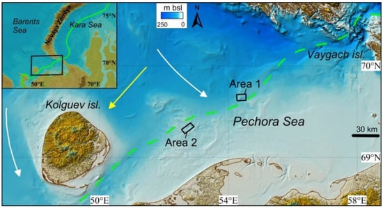
Figure 1.
Overview map of the working area and polygons of detailed research. The green line shows the supposed margin of the Late Weichselian glaciation (after [14]). Large-scale ice-flow directions (white arrows) during the LGM are indicated [9,17]. The yellow arrow shows the ice sheet flow during the LGM, inferred from the composition of glacial erratics in diamictons [7]. Bathymetry retrieved from [18].

2. Materials and Methods
A multibeam echosounding system was installed on the RV Akademik Nikolaj Strakhov in 2006. This system consists of a Reson 100 kHz SeaBat 8111, an Applanix POSMV integrating motion sensor and gyrocompass data. In addition, an EdgeTech 3300 chirp sub-bottom profiler was installed in 2006. The multibeam and sub-bottom transducers are installed in a hull-mounted gondola. The swath-bathymetric data were processed using the PDS2000 software from Teledyne. The processed data were gridded at cell sizes of 10 × 10 m, and visualizations were carried out using the PDS2000 and ArcGIS software.
In addition, the high-resolution parametric sub-bottom profiler SES-2000 Standard with frequencies of 8–10 kHz installed on the pole near the starboard was used. Sediment samples were taken using an ocean grab sampler in the area of investigations.
The surveys were carried out in two main areas located in the vicinity of the LGM ice sheet margin, inferred by [9,14], in the Pechora Sea (Figure 1).
3. Results
3.1. Seafloor Morphology and Sediments in Area 1
Submarine ridges of various sizes and orientations are mapped within Area 1 (Figure 2). In the western part, a large complex of ridges extends over an area of about 2 × 6 km (Figure 2 and Figure 3). Its relative height above the surrounding flatter seafloor is between 13 and 15 m. The shoalest point of the complex has a depth of about 40 m. The top surface and the slopes of the complex are characterized by an elaborate morphology due to the sets of ridges it comprises, which have various configurations.
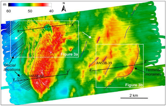
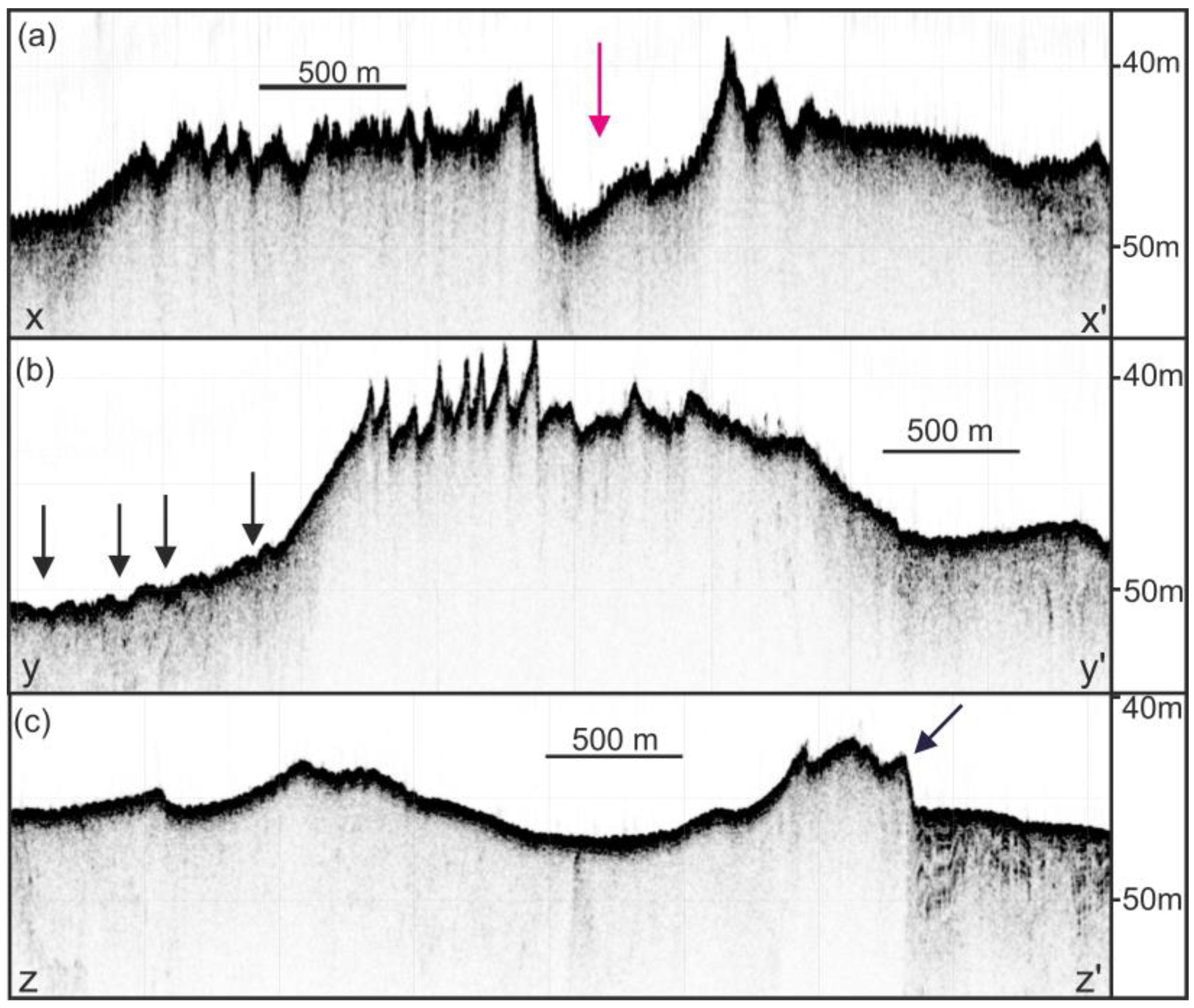
Figure 2.
Multibeam bathymetric map of Area 1 in the central part of the Pechora Sea. Sampling points are shown with black rings. White arrows indicate the ice-flow pathways inferred from the glacial landforms.

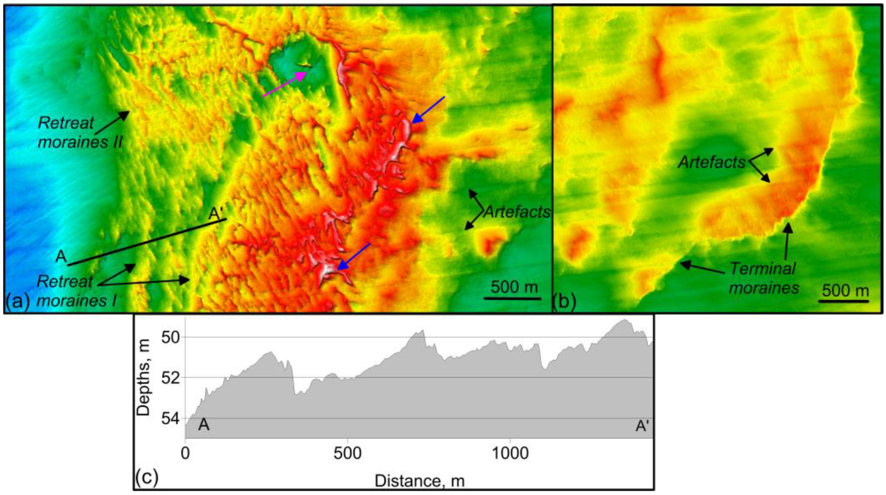
Figure 3.
(a) Detailed map of the glacial landforms mapped in the north-western part of Area 1; (b) Detailed map of the glacial landforms mapped in the south-eastern part of Area 1 (the locations are in Figure 2); (c) Bathymetric cross profile through moraines. The location is in Figure 3a. The pink arrow points to the ring structure. Blue arrows indicate possible eskers.
There are two main types of identified ridges in the western part of Area 1. The first type is represented by roughly 3 km-long and almost crescent-like subparallel ridges with an azimuth of 15°–20° (purple lines in Figure 2, Retreat moraines I in Figure 3a). These are located on the main height on the north-western side of the complex. A cross-section of these ridges shows an asymmetry with gentle western slopes and steeper eastern and south-eastern sides (Figure 3c).
The second type of moraines includes smaller ridges oriented along azimuths of 335°–340°, forming the uppermost part of the moraine complex (Retreat moraines II in Figure 3a). The relative heights of these smaller ridges are between 1 and 3 m, and their average widths at the base are about 50 m. There is a direct connection between the morphological particularities of the smaller ridges and the underlaying elevated area forming the base of the moraine complex. The smaller ridges are the features that overlay the main high of the moraine complex, and they comprise a large series of ridges.
Ridge formations of a convex semicircular shape are found on the shallower area of the complex (blue arrows in Figure 3a). This type of ridges is also characterized by an asymmetric cross-profile. Their length reaches 1 km, and the height (relief) is up to 3 m. A ring structure formed by articulated ridges of a similar type with an isometric depression in the center is apparent on the shoal (magenta arrow in Figure 3 and Figure 4a). The relative height of the sides over the bottom of the depression is 6 m, with a diameter of about 500 m.

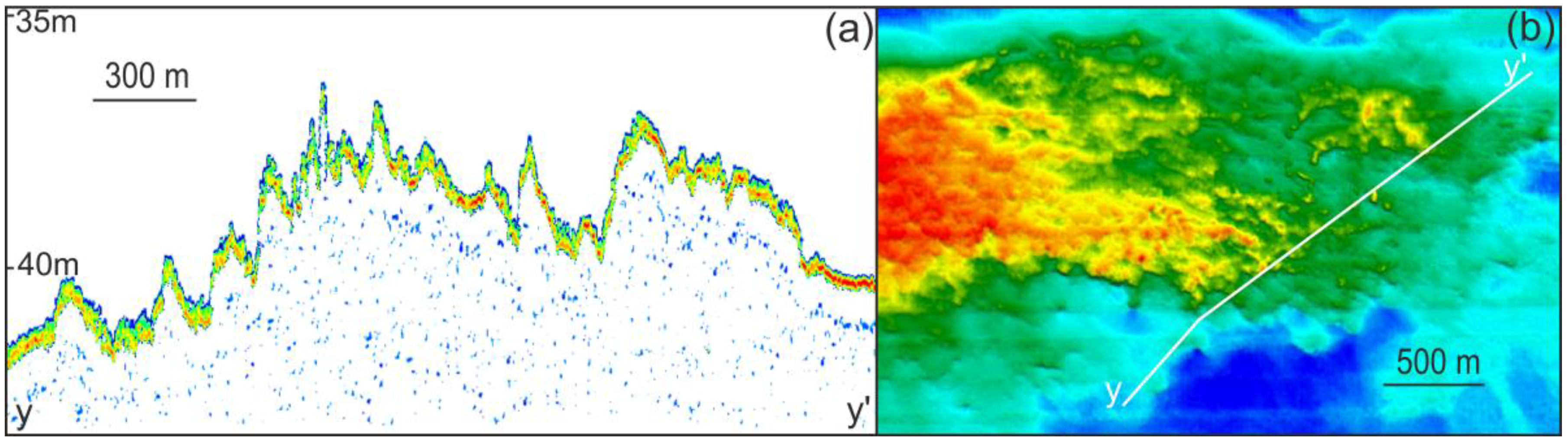
Figure 4.
Sub-bottom cross-sections through the glacial landforms mapped within Area 1; see Figure 2 for locations. Arrows point to: (a) Ring structure; (b) Glacial linear features; (c) Terminal moraine.
Glacial lineations oriented along an azimuth of 225° are identified in the bottom relief of the western part of Area 1. These lineations are not fully coherent with respect to their extent and are characterized by an incision depth of up to 0.5 m and a width of up to 50 m (black lines in Figure 2, Glacial lineations in Figure 3a).
In the central and eastern parts of Area 1, positive subparallel echelon-like features are mapped (blue lines in Figure 2). These are similar to the first type of ridges described above, but with an azimuth from 0° to 15°. They are asymmetrical, up to 4 km long, 750 m wide at their base and 5 m high (Figure 4c). The easternmost ridges are arcuate in planform (dark blue line in Figure 2).
Sediment sampling was carried out at two stations in Area 1 using a grab sampler. The retrieved sediments from these stations can be described as a diamicton. They contain rock fragments of a predominantly medium roundness, composed mainly of sandstones and siltstones ranging in size from 2 to 17 cm. Some of them are characterized by an “iron-like” shape (Figure 5). The matrix is a gray-yellow viscoplastic silty-pelitic material with a sandy admixture.
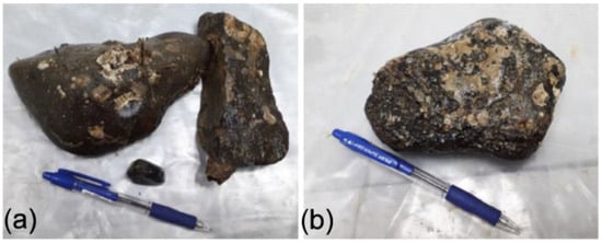
Figure 5.
Coarse material from sampling points: (a) ANS-38-39; (b) ANS-38-40. Figure 2 for locations. Pen is for scaling, 14 cm.
3.2. Seafloor Morphology and Sediments in Area 2
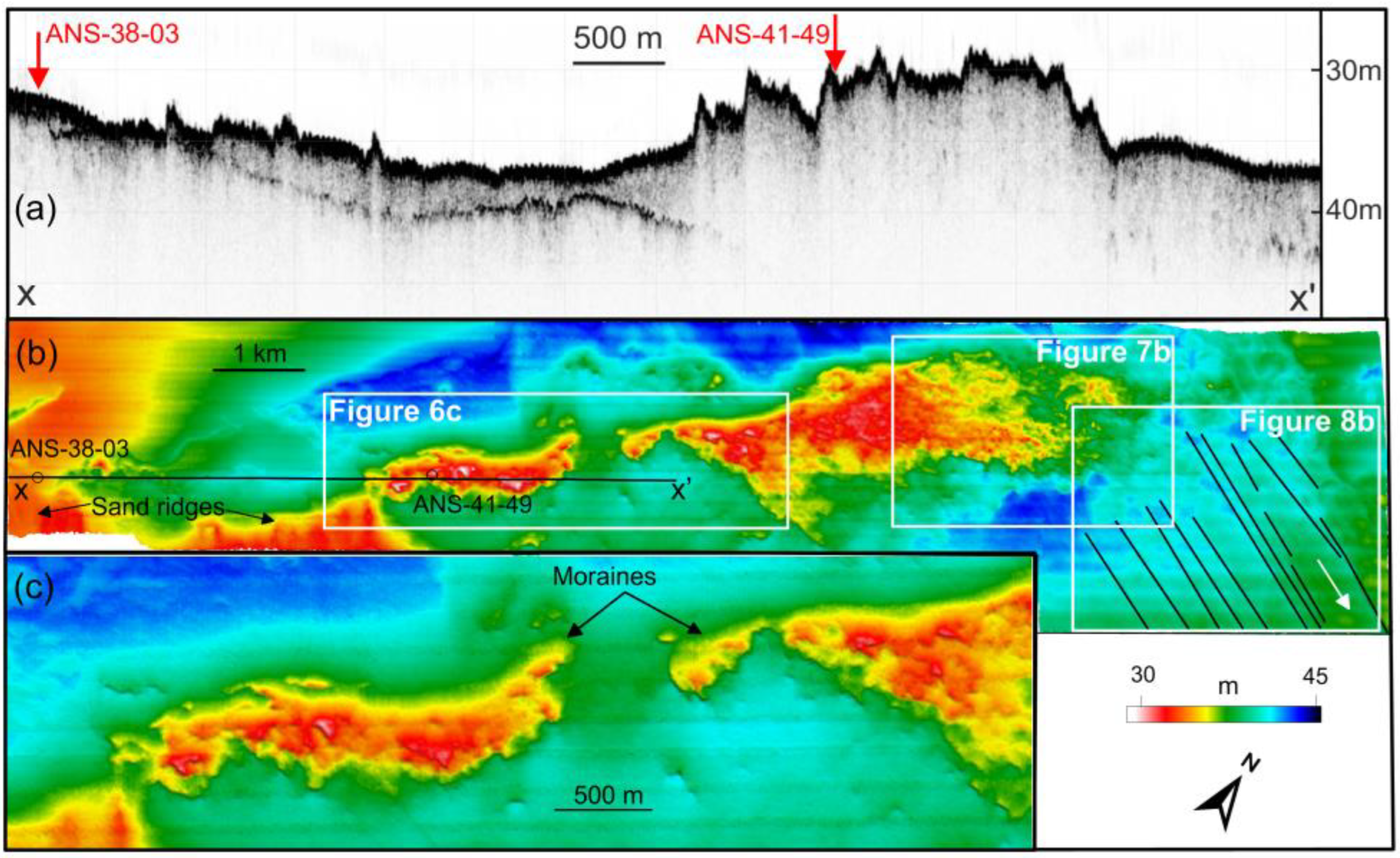
Moraines forming crescent-like elongated landforms, with reliefs up to 7 m in height, were also mapped in Area 2 (Moraines on Figure 6c). These are asymmetrical in the cross-section, with gentle eastern slopes of about 1° and steeper western slopes of about 2°–3°. They follow a general orientation along an azimuth of 280°–300°. The morphology of the moraine ridges ranges from linear to curvy (Figure 6c and Figure 7) from place to place, similar to the moraine rib-like patterns observed on the other glacial shelfs. There are several smaller ridges up to 100–150 m long, 1–2 m high and 15–20 m wide in the north-eastern part of Area 2 (Figure 7).

Figure 6.
(a) Sub-bottom cross-section; (b) Overview multibeam bathymetry of Area 2; (c) Subset of Area 2 with moraines. Sampling locations are shown: (a) with red arrows, (b) with black rings. The white arrow indicates the ice-flow pathway inferred from the glacial landforms. The black lines in Figure 6b point to glacial linear features.
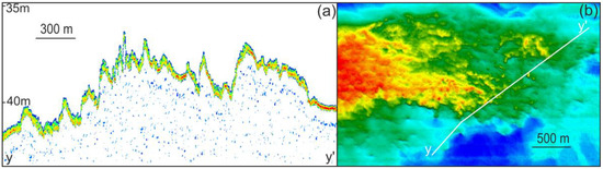
Figure 7.
(a) Cross-section obtained with the SES-2000 profiler; (b) Multibeam bathymetry of the moraine ridges mapped in the north-eastern part of Area 1. The location of the map is shown in Figure 6.
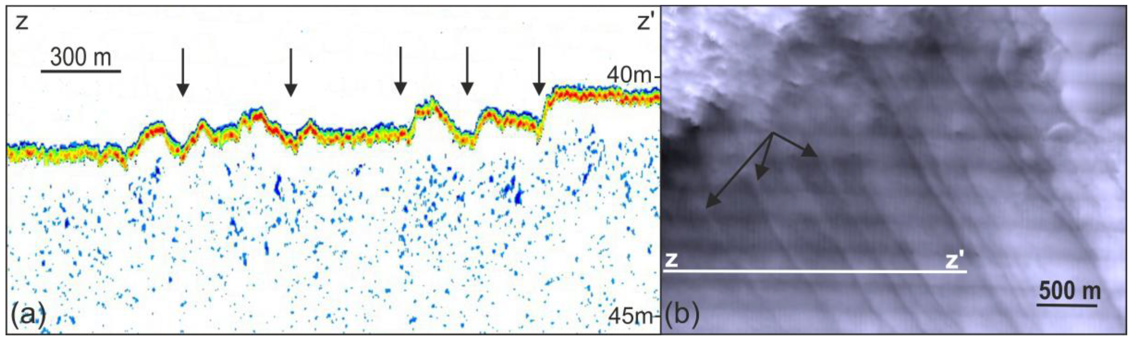
The north-eastern part of Area 2 is occupied by a plain with a gentle slope at an angle of 1° (Figure 6b). It is complicated by areas of low-amplitude undulating hilly relief. Traces of linear features, likely glacial lineations, oriented along the azimuth of 120° are mapped here at depths of 40–42 m (Figure 6b and Figure 8). The depth of the incision is up to 0.8 m, and the width is up to 150 m (Figure 8).
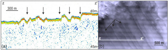
Figure 8.
(a) Sub-bottom cross-section; (b) Multibeam bathymetry from Area 2. Black arrows point to the glacial linear features. Figure 6 for the location.
Sediment sampling was carried out at two locations in Area 2 (Figure 6). Well-sorted medium-grained sands of brownish-olive color were recovered at station ANS 38-03. At station ANS 41-49, located at the moraine, a diamicton with fragments of various petrographic compositions up to 18 cm in size and with a matrix of viscoplastic silty-pelitic clays of gray colors and a slight admixture of sandy material was retrieved.
4. Discussion
The distribution of glacial landforms was mapped in two areas (Area 1 and 2) of the Pechora Sea based on our surveys in 2018–2021. Ridges mapped in both areas are characterized by a clearly expressed asymmetry of their transverse profiles (Figure 4, Figure 6a and Figure 7a), which is common for moraines [19].
It is possible to distinguish two main types of the identified ridges in the western part of Area 1, considering their morphology in the plan and in the cross-section (Figure 3a and Figure 4a,b). Both of these types of ridges are interpreted here as retreat moraines formed when material is transported by the forward-moving ice sheet to be deposited at its margin, which is overall retreating from mass loss, e.g., from calving (Figure 1). Recessional moraines of this type may also be formed by the push of material during small winter re-advances [20] and are commonly associated with a slow and steady ice retreat [19]. The ring structure on the shoalest part of the moraine complex (Figure 3a and Figure 4a) is difficult to interpret. From some aspects, it resembles the “ice-fingerprints” described in the central Barents Sea by [21]. The ice-fingerprints they mapped were interpreted to have been formed by the ploughing of sediment by advancing “fingers” of grounded ice. However, the shape of the ridge outlining the north-eastern part of the ring structure suggests, rather, that this part of the margin first retreated faster and formed an indent in the margin, which thereafter stood still, permitting a larger ridge to be formed, while the surrounding sections caught up.
Type II retreat moraines overlap type I (Figure 3a). So, they are younger in age and were likely formed as a result of subsequent oscillations of the ice sheet. The absence of type II ridges at deeper depths and their short length compared to that of type I moraines may indicate a smaller thickness and extent of the ice front in the last phases of the ice sheet advance in the area. Sets of these small transverse ridges on the seafloor are common in a relatively shallow shelf, where deglaciation takes the form of the slow retreat of a grounded tidewater glacier margin [1].
The ridge-like formations indicated by the blue arrows in Figure 3a are not straightforward to interpret. They could be eskers that have subsequently been overridden by the ice and are therefore overprinted by the retreat ridges or an incoherent terminal moraine from an earlier ice lobe. Esker systems commonly reflect the synchronous configuration of the whole subglacial hydrological system [22]. A subglacial origin is confirmed by the superimposition of sets of retreat ridges on our esker system (Figure 3a). Eskers are usually orientated approximately in the direction of past glacier flow. If these are eskers, it confirms the ice-flow pathway with the NE-SW motion vector in Area 1.
The small streamlined linear landforms located to the west of the moraine complex in Area 1 (Figure 3a and Figure 4b) are interpreted as glacial lineations formed under fast-flowing grounded ice. This type of landform is commonly considered to be formed during the deformation of subglacial sediments beneath active ice streams [23]. The lineations in Area 1 indicate a past ice-flow in the NE-SW direction, which is consistent with the previously proposed direction during the LGM in this area by [7] (Figure 1).
The arcuate ridges in the eastern part of Area 1 are interpreted as terminal moraines formed at the margin of the Barents-Kara Ice Sheet (dark blue line in Figure 2 and Figure 3b). They record the southernmost extent of the most recent continental shelf glaciation in this area. This is also indicated by the appearance of acoustically stratified layers in the sub-bottom profile section to the east of these ridges, suggesting sediment deposition in a marine non-ice-covered area for some time (Figure 4c). These stratified layers contrast with the areas of acoustically transparent sub-bottom profiles, which is typical for moraines in this area.
Terminal moraines reflect the shape of the ice edge at the time of deposition, so they are located across the movement of the ice flow. Terminal moraine ridges in submarine glacier-influenced environments are usually asymmetrical, with a steeper ice distal face [24]. This suggests the NW-SE direction of the ice-flow pathway in this area (Figure 1).
The sediment samples from the areas where we inferred moraines based on the geophysical mapping support our interpretation. Diamictons in the Pechora Sea have, from previous studies, been shown to be comprised of coarse clasts and inclusions of bedrock, with an additional amount of gravel and sand of various sizes [25]. Samples collected in Area 1 (ANS-38-39 and ANS-38-40, Figure 2) and Area 2 (ANS-41-49, Figure 6b) were composed of unsorted material, i.e., typical diamicton-type sediments with coarse components (Figure 5).
At the sampling site ANS-38-03 (Figure 6b) well-sorted sands were retrieved. It should be noted that the surface sediments of the region adjacent to Area 2 are mainly represented by Holocene sands of various sizes [26]. The development of the sand ridges found in Area 2 (Figure 6b) is probably due to the inherent instability of the seabed under the influence of currents.
The crescent-like elongated ridges in Area 2 (Figure 6) are interpreted as moraines. The direction of their orientation (SE-NW) indicates that they were formed during still-stands in ice sheet retreat during the last deglaciation. The small-scale ridges found in the north-eastern part of Area 2 (Figure 7) are probably small retreat moraines. It is difficult to determine the orientation of these landforms from multibeam data (Figure 7b). It seems that they are “smeared” and partially destroyed by post-glacial erosion, probably due to the active lithodynamic processes in the region.
The parallel, streamlined landforms mapped in the northeastern part of Area 2 are interpreted as glacial lineations (Figure 8). They are similar in dimensions to elongate landforms interpreted as mega-scale glacial lineations (MSGLs) from many Late Quaternary glacier-influenced environments [27]. The orientation of MSGLs in Area 2 indicates ice flow in the NW–SE direction (Figure 6).
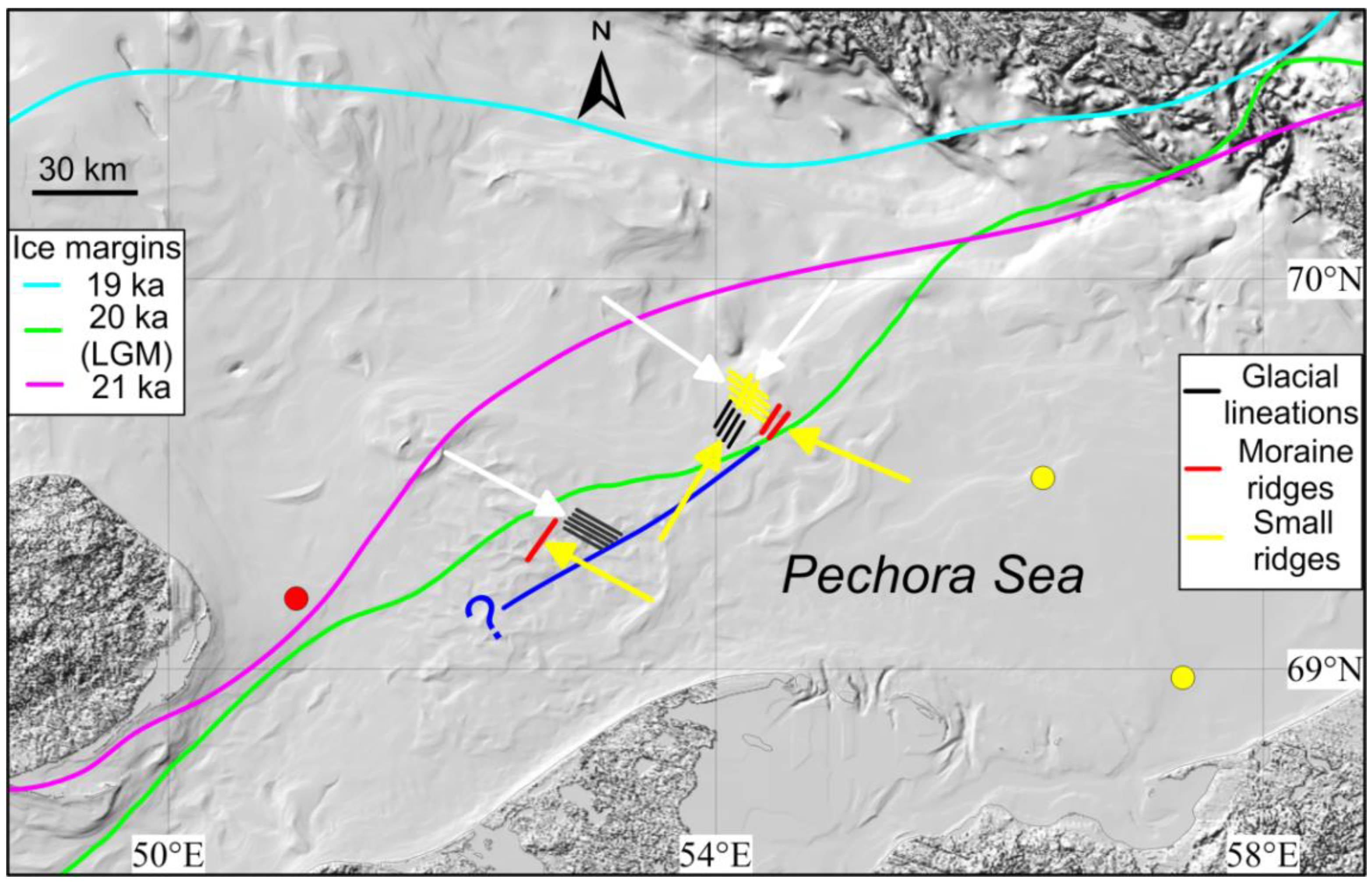
We have mapped the distribution of submarine glacial landforms in the Pechora Sea based on the findings from Areas 1 and 2 (Figure 9). The reconstruction of the ice margins of the Late Weichselian ice sheet (Figure 9) [28] allowed us to trace their dynamics and determine the dates of deglaciation of the Pechora Sea. The deglaciation started after 20 ka (LGM). By 19 ka, most of the Pechora Sea was ice-free (Figure 9).

Figure 9.
Distribution of submarine glacial landforms identified in the Pechora Sea. Reconstruction of the margins of the Late Weichselian ice sheet for the 21 ka, 20 ka and 19 ka BP taken from [28]. White arrows indicate the ice-flow pathways inferred from our data. Yellow arrows indicate the ice-retreat directions. The circles indicate the location of the dated cores [7]. The blue line is the minimum extent of the south-eastern margin of the Barents–Kara ice sheet during the LGM, based on our data.
Our study revealed glacial landforms of various orientations, suggesting a slightly more local complex scenario of inherent phases of the advance and retreat of the ice sheet. Ice flow directions from two main sources were registered in Area 1.
The terminal moraines and probable eskers mapped in Area 1 indicate an early phase of ice flowing from the central part of the Barents Sea in the NW–SE direction (Figure 9). This large-scale ice flow direction was previously assumed [9,17] (Figure 1). MSGLs indicate an early phase which is characterized by relatively fast flowing ice in the NE–SW direction. This ice flow direction was inferred earlier from the composition of glacial erratics in diamictons [7,25] (Figure 1). The ice sheet of the Barents Sea during the last glaciation was in contact with the ice sheet of the Kara Sea. The ice flow of the NE-SW direction was probably formed from this confluence zone in the Novaya Zemlya region [29].
Differences in the orientation of the retreat ridges I and II (Figure 3a) on the moraine complex indicate the multidirectional nature of the movement of glacial masses and allow us to determine two ice-retreat directions in a later phase (yellow arrows in Figure 9, SE-NW and SW-NE). It agrees well with the recognized reconstructions (arrows in Figure 1) considering the direction of the ice flow, which is roughly opposite to the direction of the ice retreat.
In Area 2, the occurrence of MSGLs suggests an early phase of ice flowing dominated by dynamic conditions with fast ice. Retreat moraines and a lack of fast flow indicators in the north-western part of Area 2 suggest a later phase characterized by a slower ice retreat in the SE–NW direction (yellow arrow in Figure 9).
The absolute age of the mapped glacial landforms is unknown. However, five major seismostratigraphic units, SSU-I–V, were recognized earlier in the Pechora Sea; two of them are diamictons [8]. The Late Weichselian diamicton layer forms the seismostratigraphic unit SSU-III. The oldest Middle Weichselian diamicton layer forms SSU-V [8]. Recently, new isopach map of SSU-III has been compiled for the Pechora Sea, based on a large volume of seismic and drilling data [30]. According to these data, SSU-III can be traced confidently in our study area and has a thickness of at least 10 m. Based on these data, we assume that the mapped glacial landforms belong to this upper diamicton layer. Thus, despite the limited age control of the mapped glacigenic bedforms, we suggest that the landforms presented and discussed here were formed during the LGM and the subsequent deglaciation.
A few radiocarbon dates are available to provide dating control in the Pechora Sea [7]. In the eastern part of the Pechora Sea, layers of diamicton overlain by thick marine sediments were sampled in two sites (yellow circles in Figure 9). A series of 14C dates collected from these fine-grained marine sediments yielded consistent ages from about 40 ka and onwards (Figure 3), proving that the underlying diamicton is Middle Weichselian in age [7].
Two superimposed diamictons separated by an interglacial unit were revealed in a borehole near Kolguev Island (red circle in Figure 9). Based on the 14C dates obtained above and below the LGM diamicton, we can assume that this site was occupied by the ice during the last glaciation [7].
The geographic boundary between the two types of stratigraphy described above has been interpreted to reflect the south-eastern margin of the Barents-Kara Ice Sheet during the LGM [7,31] (Figure 9). The exact boundary of the distribution of the last glaciation in the Pechora Sea will be located between the drilling points described above (circles in Figure 9). It should be noted that the coastal sections further south from our study area are characterized by non-glacial aeolian sediments and ice wedges, indicating that this area was not overrun during the last glacial advance [32].
At present, the leading point of view is that the entire Barents Sea without the southern part of the Pechora Sea was covered with a continuous ice sheet during the LGM [7,14]. The mapped glacial landforms clearly indicate that an ice sheet extended over the area, while the Pechora basin, at the same time, comprised lowland characterized by a cryogenic subaerial landscape. As a result of our study, the minimum extent of the south-eastern margin of the Barents-Kara ice sheet during the LGM was determined (Figure 9). It should be noted that the glaciation boundary to the west and south of this area has yet to be resolved. Some researchers point to the existence of a network of paleovalleys in the western part of the Pechora Sea [10,33]. We have not identified terminal moraines in Area 2, so the possibility of the existence of ice-marginal landforms to the south of the established extent is not excluded. Detailed geophysical mapping and dating of key stratigraphic units are needed to definitively determine the ice sheet configuration and past ice-flow directions during the glaciation in this area.
Author Contributions
Conceptualization, S.N. and R.A.; validation, S.N., M.J. and Y.Z.; formal analysis, N.S. and I.C.; investigation, S.S., N.D., E.S., Y.Z. and A.R.; resources, S.N. and N.S.; data curation, E.M., E.S., Y.Z. and A.R.; writing—original draft preparation, S.N., E.M. and S.S.; writing—review and editing, R.A. and M.J.; visualization, R.A. and E.M.; supervision, S.N. and M.J.; project administration, R.A. and I.S.; funding acquisition, N.S. and I.S. All authors have read and agreed to the published version of the manuscript.
Funding
This work was performed in the framework of the state assignments of the Shirshov Institute of Oceanology RAS (theme no. FMWE-2021-0005) and the Geological Institute RAS (theme no. FMUN-2019-0076), supported by Tomsk State University as a part of Program Prioritet 2030, run by the Ministry of Science and Education of the Russian Federation.
Data Availability Statement
Not applicable.
Acknowledgments
We thank the crew of the R/V Akademik Nikolaj Strakhov for their participation and help in the field research.
Conflicts of Interest
The authors declare no conflict of interest.
References
- Dowdeswell, J.A.; Canals, M.; Jakobsson, M.; Todd, B.J.; Dowdeswell, E.K.; Hogan, K.A. The variety and distribution of submarine glacial landforms and implications for ice-sheet reconstruction. Geol. Soc. Lond. Mem. 2016, 46, 519–552. [Google Scholar] [CrossRef]
- Nikiforov, S.; Koshel, S. Seabed Morphology of the Russian Arctic Shelf; Nova Science Publishers, Inc.: Hauppauge, NY, USA, 2010; p. 122. [Google Scholar]
- Jakobsson, M.; Andreassen, K.; Bjarnadóttir, L.R.; Dove, D.; Dowdeswell, J.A.; England, J.H.; Funder, S.; Hogan, K.; Ingólfsson, Ó.; Jennings, A.; et al. Arctic Ocean glacial history. Quat. Sci. Rev. 2014, 92, 40–67. [Google Scholar] [CrossRef]
- Pavlidis, Y.; Ionin, A.; Shcherbakov, F. Arctic Shelf: Late Quaternary History as a Base for Evolution Prognosis; GEOS: Moscow, Russia, 1998; p. 187. (In Russian) [Google Scholar]
- Pavlidis, Y.; Polyakova, E. Late Pleistocene and Holocene depositional environments and paleooceanography of the Barents Sea: Evidence from Seismic and Biostratigrapic data. Mar. Geol. 1997, 143, 189–205. [Google Scholar] [CrossRef]
- Grosswald, M. New Approach to the Ice Age Palaeogydrlogy of Nothern Eurasia. In Palaeohydrology and Environmental Change; Wiley: Chichester, UK, 1998; pp. 199–214. [Google Scholar]
- Polyak, L.; Gataullin, V.; Okuneva, O.G.; Stelle, V. New constraints on the limits of the Barents-Kara ice sheet during the Last Glacial Maximum based on borehole stratigraphy from the Pechora Sea. Geology 2000, 28, 611–614. [Google Scholar] [CrossRef]
- Gataullin, V.; Mangeroud, J.; Svendsen, J.I. The Extent of the late Weichselian Ice Sheet in the Southeastern Barents Sea. Glob. Planet. Change 2001, 31, 453–474. [Google Scholar] [CrossRef]
- Svendsen, J.I.; Gataullin, V.; Mangerud, J.; Polyak, L. The glacial history of the Barents and Kara Sea region. In Developments in Quaternary Sciences; Ehlers, J., Gibbard, P.L., Eds.; Elsevier: Amsterdam, The Netherlands, 2004; Volume 2, Part 1, pp. 369–378. [Google Scholar]
- Pavlidis, Y.; Nikiforov, S.; Ogorodov, S.; Tarasov, G. The Pechora Sea: Past, Recent, and Future. Oceanology 2007, 47, 865–876. [Google Scholar] [CrossRef]
- Gusev, E.; Artemieva, D. Problems of mapping and genetic interpretation of Quaternary sediments of the Arctic. In Proceedings of the VI International Conference of Young Scientists and Specialists “New in Geology and Geophysics of the Arctic, Antarctic and World Ocean”, Saint Petersburgh, Russia, 25–27 April 2018; pp. 21–22. (In Russian). [Google Scholar]
- Chuvardinsky, V. The Problem of Ice Cover Glaciers of the Arctic and Subarctic; Lambert: Moscow, Russia, 2016; p. 204. (In Russian) [Google Scholar]
- Krapivner, R. Crisis of the Glacial Theory: Arguments and Facts; GEOS: Moscow, Russia, 2018; 320 p. (in Russian) [Google Scholar]
- Svendsen, J.I.; Alexanderson, H.; Astakhov, V.I.; Demidov, I.; Dowdeswell, J.A.; Funder, S.; Gataullin, V.; Henriksen, M.; Hjort, C.; Houmark-Nielsen, M.; et al. Late Quaternary ice sheet history of Northern Eurasia. Quat. Sci. Rev. 2004, 23, 1229–1271. [Google Scholar] [CrossRef]
- Nikiforov, S.L.; Sorokhtin, N.O.; Dmitrevskiy, N.N.; Ananiev, R.A.; Sokolov, S.Y.; Ambrosimov, A.K.; Meluzov, A.A.; Mutovkin, A.D. Researches in cruise 38 of the R/V Akademik Nikolaj Strakhov in the Barents sea. Oceanology 2019, 59, 801–802. [Google Scholar] [CrossRef]
- Nikiforov, S.L.; Ananiev, R.A.; Dmitrevskiy, N.N.; Sorokhtin, N.O.; Moroz, E.A. Geological and Geophysical Studies on Cruise 41 of the R/V Akademik Nikolaj Strakhov in Arctic Seas. Oceanology 2020, 60, 295–296. [Google Scholar] [CrossRef]
- Larsen, E.; Andreassen, K.; Nilssen, L.C.; Raunholm, S. The Prospectivity of the Barents Sea: Ice Ages, Erosion and Tilting of Traps; Geological Survey of Norway: Trondheim, Norway, 2003; p. 60. [Google Scholar]
- Nikiforov, S.; Koshel, S.; Libina, N. Digital elevation models of the White and Barents seas. Geoinformatics 2018, 2, 32–36. (In Russian) [Google Scholar]
- Ottesen, D.; Dowdeswell, J.A. An inter-ice-stream glaciated margin: Submarine landforms and a geomorphic model based on marine-geophysical data from Svalbard. Geol. Soc. Am. Bull. 2009, 121, 1647–1665. [Google Scholar] [CrossRef]
- Boulton, G.S. Push-moraines and glacier-contact fans in marine and terrestrial environments. Sedimentology 1986, 33, 667–698. [Google Scholar] [CrossRef]
- Bjarnadóttir, L.R.; Winsborrow, M.C.M.; Andreassen, K. Deglaciation of the central Barents Sea. Quat. Sci. Rev. 2014, 92, 208–226. [Google Scholar] [CrossRef]
- Brennand, T.A. Deglacial meltwater drainage and glaciodynamics: Inferences from Laurentide eskers, Canada. Geomorphology 2000, 32, 263–293. [Google Scholar] [CrossRef]
- Stokes, C.R.; Clark, C.D. Geomorphological criteria for identifying Pleistocene ice streams. Ann. Glaciol. 1999, 28, 67–74. [Google Scholar] [CrossRef]
- Benn, D.I.; Evans, D.J.A. Glaciers and Glaciation, 2nd ed.; Hodder: London, UK, 2010. [Google Scholar]
- Epshtein, O.; Romanyuk, B.; Gataullin, V. Pleisctocene Scandinavian and Novaya Zemlya Ice Sheets in the Southern Barents Sea and Northern Russian Plain. Byull. Komis. Izuchen. Chetvert. Perioda 1999, 63, 132–155. (In Russian) [Google Scholar]
- Epshtein, O.; Dlugach, A.; Starovoytov, A. Main features of the structure, litological composition, and thickness of the quaternary deposits cover in the eastern Barents Sea. Dokl. Earth Sci. 2019, 485, 331–334. [Google Scholar] [CrossRef]
- Spagnolo, M.; Clark, C.D.; Ely, J.C.; Stokes, C.R.; Anderson, J.B.; Andreassen, K.; Graham, A.G.; King, E.C. Size, shape and spatial arrangement of mega-scale glacial lineations from a large and diverse dataset. Earth Surf. Process. Landf. 2014, 39, 1432–1448. [Google Scholar] [CrossRef]
- Hughes, A.L.; Gyllencreutz, R.; Lohne, Ø.S.; Mangerud, J.; Svendsen, J.I. The last Eurasian ice sheets—A chronological database and time-slice reconstruction, DATED-1. Boreas 2016, 45, 1–45. [Google Scholar] [CrossRef]
- Landvik, J.Y.; Bondevik, S.T.E.I.N.; Elverhøi, A.N.D.E.R.S.; Fjeldskaar, W.I.L.L.Y.; Mangerud, J.A.N.; Salvigsen, O.T.T.O.; Siegert, M.J.; Svendsen, J.I.; Vorren, T.O. The Last Glacial Maximum of Svalbard and the Barents Sea area: Ice sheet extent and configuration. Quat. Sci. Rev. 1998, 17, 43–75. [Google Scholar] [CrossRef]
- Epshtein, O.; Dlugach, A.; Starovoytov, A. Cover of the last glaciation deposits in the Eastern Barents Sea: Specificity of composition, thickness distribution, immensity, and peculiarity of structural forms. Dokl. Earth Sci. 2019, 487, 898–901. [Google Scholar] [CrossRef]
- Polyak, L.; Niessen, F.; Gataullin, V.; Gainanov, V. The eastern extent of the Barents-Kara ice sheet during the Last Glacial Maximum based on seismic-reflection data from the eastern Kara Sea. Polar Res. 2008, 27, 162–174. [Google Scholar] [CrossRef]
- Mangerud, J.; Astakhov, V.; Svendsen, J.I. The extent of the Barents–Kara ice sheet during the Last Glacial Maximum. Quat. Sci. Rev. 2002, 21, 111–119. [Google Scholar] [CrossRef]
- Lastochkin, A. Underwater valleys of the northern shelf of Eurasia. Izv. All-Union Geogr. Soc. 1977, 109, 412–417. (In Russian) [Google Scholar]


Disclaimer/Publisher’s Note: The statements, opinions and data contained in all publications are solely those of the individual author(s) and contributor(s) and not of MDPI and/or the editor(s). MDPI and/or the editor(s) disclaim responsibility for any injury to people or property resulting from any ideas, methods, instructions or products referred to in the content. |
© 2023 by the authors. Licensee MDPI, Basel, Switzerland. This article is an open access article distributed under the terms and conditions of the Creative Commons Attribution (CC BY) license (https://creativecommons.org/licenses/by/4.0/).