Abstract
Scanlines constitute a robust method to better understand in 3D the fracture network variability in naturally fractured geothermal reservoirs. This study aims to characterize the spacing variability and the distribution of fracture patterns in a fracture granitic reservoir, and the impact of the major faults on fracture distribution and fluid circulation. The analogue target named the Noble Hills (NH) range is located in Death Valley (DV, USA). It is considered as an analogue of the geothermal reservoir presently exploited in the Upper Rhine Graben (Soultz-sous-Forêts, eastern of France). The methodology undertaken is based on the analyze of 10 scanlines located in the central part of the NH from fieldwork and virtual (photogrammetric models) data. Our main results reveal: (1) NE/SW, E/W, and NW/SE fracture sets are the most recorded orientations along the virtual scanlines; (2) spacing distribution within NH shows that the clustering depends on fracture orientation; and (3) a strong clustering of the fracture system was highlighted in the highly deformed zones and close to the Southern Death Valley fault zone (SDVFZ) and thrust faults. Furthermore, the fracture patterns were controlled by the structural heritage. Two major components should be considered in reservoir modeling: the deformation gradient and the proximity to the regional major faults.
1. Introduction
In deep geothermal systems, many studies have been undertaken to better understand the importance of the natural fractures in various contexts [1,2]. In granitic basement rocks, the permeability is mostly increased by the fracture network and faults [3,4,5,6,7], while the porosity is increased by both the alteration (e.g., dissolution of primary minerals) and the proximity to fracture zones ([8], this issue). The low rock matrix permeability and porosity allow the fluid flow within fracture networks [9,10,11]. The understanding of the spatial arrangement of the fracture network constitutes the main issue in fractured reservoirs [1,3,7,12,13].
A fracture network is characterized by geometrical parameters such as lengths, spacings, widths, orientations, fracture distributions, and the relationships between them significantly affect the connectivity within the reservoir [9,14,15,16,17]. Among these parameters, spacing between fractures is a well-considered parameter, because it controls the probability of intersecting fractures during drilling [18]. Statistic parameters that describe fracture spacing include: (1) The mean, which characterizes the global expected frequency of fracture intersection, and (2) the standard deviation, which describes the distribution of the fractures around the mean.
Regarding the spacing distribution, fractured zones can be classified into: (1) Fracture corridor, a term usually used for a dominant set of fractures displaying an important variation of fracture intensity. It can represent the main drains for fluid circulation in various reservoir contexts such as geothermal fields [19]; (2) fracture arrays, a term generally used to define a dominant set of fractures which forms an angle to the swarm (area in which any kind of fracture appears) [20]; (3) shear zone, which is defined as a continuous deformed zone with a high strain [21], accommodated by a cataclastic process in granitic rocks and crystalline plasticity in (e.g., carbonate rocks); and (4) fault zone characterized by a fault and its associated damage zone which can act as a barrier or a drain for flow, depending on its intrinsic properties [5,20,22]. In crystalline basement rocks, the fracture distribution within the damage zone is influenced by the distance from the fault core and its displacement along the fault plane [23]. Indeed, the strong variation in fracture distribution (fracture densities) is commonly observed near active faults. Ostermeijer et al. [23] add that the pattern is mainly ruled by the distribution of macro-damage induced on shear-accommodating subsidiary fractures.
Spatial organization of fracture systems became an important studied topic in the recent decades because of the necessity to better understand the architecture of fractured reservoirs [7,24,25,26]. The spatial arrangement can be quantified using statistical laws (e.g., power law, log normal, and exponential law) [24,27,28] or statistical parameters, such as the coefficient of variability (Cv) along 1D [20] and the normalized correlation count method [27]. The main goal is to enhance the fracture distribution understanding (clustered, random, or uniform distribution) and its effects on connectivity [29]. In that case, many studies are focused on fracture networks characterization in various settings and at different scales [3,12,16,20,30,31]. They commonly used field analogues at surface to resolve the challenge of lack of sub-surface information in reservoirs [32]. The characterization of heterogeneity of the fracture spacing and the fracture abundance at any scale may be performed using line sampling method along one dimension (1D) named scanline (e.g., [26]). The present study combines the spacing data of joints (opening-mode fractures), veins (partially or fully filled), and faults to highlight the spatial arrangement of the fracture patterns in granitic rocks and the influence of the regional major faults. In the present study, the measured fractures, whatever their filling have been classified according to their orientation.
The present work is part of the European MEET project (multidisciplinary and multi-context demonstration of EGS exploration and exploitation techniques and potentials, [33]). This study proposes to (1) describe fracture system distribution at outcrop scale, based on fracture network parameters; (2) shows the role of the regional major faults proximity on the fracture patterns evolution in the basement rocks; and (3) highlights the impact of the deformation at outcrop scale. The present study was performed in the desert environment of Noble Hills (NH) fractured granitic basement, located in the southern termination of Death Valley (Death Valley, CA, USA), and is considered as a paleo geothermal analogue of the Upper Rhine Graben (URG, Alsace area situated in the eastern of France) ([25,34,35], this issue) geothermal systems producing electricity, because of the similarities in the basement rock nature (granite), hydrothermal alterations and the trans-tensional tectonic setting [25,34,35,36]. However, the geological history of the NH range is rather different from that of to those in the URG, but numerous pieces of evidence of analogy have been highlighted by recent work of Klee et al., [37], which addressed a list of similarities between the URG reservoir targets (exploited geothermal present-day reservoir) and the NH ranges:
- Pervasive alteration of the NH granite;
- Ubiquitous argillic alteration affecting plagioclase and biotite is present;
- Unaltered K-feldspar;
- Porosity is enhanced by the alteration and microfracturing;
- Evidence of the hydrothermal fluid percolation, as identified in an exploited geothermal reservoirs;
- Fluid circulation in open system such as in EGS systems (input of potassium and carbonates).
Based on scanline methodology (e.g., [26]), this work has been performed using a spacing measurement, compiled from four different canyons located in the central part of NH. This central part has been characterized as having a distinct spatial arrangement of fractures at different scales in comparison with the northeast and southeast parts (for additional explanations, see [25]). The scanlines are located in the granitic part of the NH range, the so called crystalline basement slice (CBS) according to Brady et al. [38]. Some of the measures were acquired directly from the field and others from virtual scanlines (method detailed in Section 3.2). Apertures of fractures have also been measured directly in the field. Numerous fractures were filled by newly formed minerals such as carbonates, oxides, and sometimes barite.
In this study, scanline methodology and statistical tools are used to better understand the fracture spacing variability and the distribution of fracture patterns at depth. This allows better characterizing reservoirs in response to the developing geothermal exploration and exploitation by EGS in basement rock context. This study was conducted:
- Through a description of the fracture system using orientation, density, spacing and aperture parameters;
- By highlighting the role of the proximity to the regional major faults on the fracture patterns;
- By highlighting the role of the deformation gradient and structural heritage at outcrop scale.
2. Geological Setting
The NH structurally belongs to the DV region (Figure 1a), which is characterized by a complex tectonic history (e.g., [39]), starting with late Cenozoic extensional and trans-tensional structures which overprint the Mesozoic to Early Cenozoic contractional structures [39,40,41]. The extensional regime of the DV has begun around 16 Ma [42,43], and is shifted to a trans-tensional regime around 5 Ma [39,44,45,46]. Recent work by Pavlis and Trullenque, [36] reconsider the age of the transcurrent deformation in DV around 12 Ma.
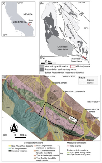
Figure 1.
(a,b) Location and geological setting of DV and NH studied area modified after [50], NDVFZ: Northern Death Valley Fault Zone, SDVFZ: Southern Death Valley Fault Zone, GFZ: Garlock fault zone, CA: California, NV: Nevada, IH: Ibex Hills, SPH: Saddle Peak Hills. (c) Structural scheme of the NH range performed thanks to high-resolution digital mapping techniques (see below) modified after [34,47]. Additional digitized fractures were obtained using orthophotos. NHFs: Noble Hills formations.
The NH ranges forms the principal physiographic feature aligned with segments of the right-lateral Southern Death Valley Fault Zone (SDVFZ) [25,47] (Figure 1b). The SDVFZ net dextral strike-slip displacement has been estimated around 40–41 km [36]. A whole compressional region was created by the interaction between the SDVFZ and the Garlock Fault (GF) system (see Figure 1b for location), which leads to shortening within the Avawatz Mountains (Figure 1b) [48,49,50].
The exhumation history of NH range is poorly described in the literature. Based on KI/temperature of illite crystals, recent work by Klee et al. [37] highlighted that the southeastern of NH is much elevated, with a higher temperature which could indicate that the south-eastern part of NH was buried deeper than its north-western part and has been exhumed.
Recent work by Chabani et al., [25] highlights the structural organization of the NH range according to the orders of fault magnitude classification by analyzing 2D maps at different scales. These orders consist in (1) second order scale, referring to the faults comprised between 20 and 30 km length; (2) third order scale, referring to faults around 10 km length; and (3) fourth order, referring to the faults under 1 km length. The first order referring to the crustal faults (higher than 100 km length) is not observed within the NH range.
The SDVFZ trending NW/SE and the GFZ trending E/W controlled NH range geometry. Indeed, the SDVFZ controls the NH geometry at large scale within the second order scale, while the GFZ trending E/W controls the NH geometry within the third order scale. Chabani et al., [25] add that the NH are divided into three internal structural domains: (1) Domain A, to the north, is characterized by the dominance of the NW/SE direction at the fourth order scale; (2) domain B, central, is marked by the dominance of the E/W and the NW/SE directions at respectively the fourth and third order scales; and (3) domain C, to the south, is also characterized by the E/W and NW/SE directions dominance but at the third and fourth order scales, respectively.
Numerous episodes of deformations have been highlighted during the fieldwork campaigns. Indeed, the SDVFZ fault segments act with a dextral movement (black lines in Figure 2b), highlighting an intense deformation with local evidences of extreme shearing. These structures are contemporaneous with the syn-kinematic dextral strike faults (orange lines in Figure 2b), highlighted in the recent work done by Klee et al. [8]. In addition, compressional structures like thrust faults crosscut outcrops 6 and 8 (red lines in Figure 2b). A clear overprinting has been recognized between SDVFZ (which also crosscut the OT2, OT6, and OT7) and the compressive structures are due to the GFZ, which acts with a sinistral movement. Furthermore, the thrusting highlighted in the present study postdates the activity of the SDVFZ. According to Chabani et al. [25], it is tempting to relate the thrust structures to the activity along the frontal termination of GFZ. Furthermore, the compressive structures are related to the interaction of the NH ranges with the Avawatz mountains during the GFZ movement.
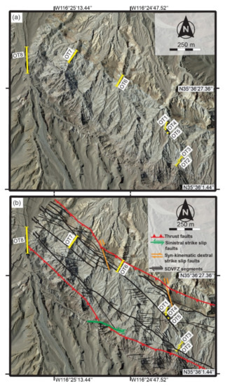
Figure 2.
(a) Map highlighting the structural position of the central part of NH, including the outcrops (OT) location and (b) SDVFZ segments position in black, syn-kinematic dextral strike slip faults in orange, sinistral strike-slip faults in green lines, and thrust faults in red. Dextral strike slip faults are syn-kinematic with SDVFZ episode, those systems are followed by thrust faults, which are contemporaneous with the GFZ orientated globally E/W.
A gradient of deformation has been highlighted in the central part of NH, with evidence of extreme shearing, close to OT6 and OT7. Boudinage structures and brittle shearing are highlighted within the Crystal Spring series (pCu, Figure 1c). In that case, the new geological map (Figure 1c) built using the high-resolution mapping techniques on the ground, using a tablet and QGIS software by Klee et al. [34] revealed a stacking of the Crystal Spring series, intruded by the Mesozoic granite (Mzla, Figure 1c). Laterally, the thickness of Crystal Spring series was reduced, as they were dragged and stretched against the granite due to the SDVFZ activity, especially in OT6 to OT8 areas.
Cenozoic volcanic series have also been highlighted in the southeastern end of the NH [47]. Cenozoic formations have been characterized by Niles, [47] outside the center part of the NH. They are mainly composed of fanglomerate, alluvial fan deposits, lacustrine deposits, sabkha, evaporitic rocks, carbonate units, and megabreccia.
3. Methodology
Scanlines are commonly used to describe the reservoir properties and the fracture systems from analogues of hydrocarbon and groundwater reservoirs [20,30,51,52,53,54], and of geothermal reservoirs [55]. The scanline methodology, widely described in the literature [2,26,54,56], helps the understanding of the fractured reservoir geometry.
3.1. Scanline Data Acquisition
In the present work, the geometrical parameters of fractures, such as orientation, spacing, and aperture, were acquired directly from scanlines in the field. A decameter was installed horizontally along the outcrop (Figure 2a). Note that data about every fracture (e.g., joint, vein or fault) intersected by the scanline were collected, whatever its orientation class or filling. The cross-cutting relationships between the studied fractures are difficult to observe in the field, as intersections rarely occur along the scanline. Then, the fracture parameters were acquired by reporting the successive position of each fracture along the scanline. The projected positions were then collected and reported in Excel software v.2019. The spacing between two consecutive fractures is given by [20]:
SA = Pn − Pn-1
SA is the apparent spacing of fractures calculated from the fracture positions measured from field, Pn refers to the position of fracture n, and Pn-1 refers to the position of fracture n–1, both expressed in meters, the location of the beginning of the measurement line being the reference. During the data analysis step, the fractures were filtered by orientation classes in order to discuss the effect of the regional directions on the local fracturing heterogeneity.
One to two scanlines were acquired from each outcrop. Five scanlines were performed along the outcrops OT 1, OT2, and OT3.
Fracture spacings were also calculated from virtual scanlines based on photogrammetric models and on fracture maps. The photogrammetric models were performed using two drones: 3DR Solo drone and DJI Phantom. These drones were loaned by University of Texas at El Paso (UTEP), TX, USA. The videos were recorded between the late morning and the early afternoon during seven consecutive days using a manual mode camera setting to reduce the effects of lighting condition. Then, pictures were extracted from the recorded videos. To provide a sufficient overlapping, pictures were extracted every second using ffmpeg software v.4.5 (Grenoble, France). The alignment of the pictures was done in Agisoft Metashape software 2020, v.1.6.5. (Saint Petersburg, Russia). Regarding the picture resolution, we ensured that every picture had a resolution of 300 dpi (300 pixels per 300 pixels). That permitted us to digitize the maximum number of fractures of decimeter length. The size of the pixel is 10 cm per pixel.
Several processing steps were needed to build the 3D models, starting by sky removal to reduce the noises, and the creation of different picture chunks (Figure 3). The 3D models were georeferenced and then imported in open access QGIS® software 2018, v.2.18.17 (Beaverton, OR, USA) to start the fracture extraction process. To improve the accuracy, ground control points (GCP) put in the field, using differential global positioning system (DGPS) and global positioning system (GPS) integrated directly in the drones, have been used. The georeferencing of each outcrop was realized independently using DGPS. The extraction of fractures was done manually by tracing every plane from the 3D outcrop. The orientation of every extracted trace plane was done automatically, and then compiled. For further explanation, the methodology of the modeling and the fracture extraction is detailed in Chabani et al. [35]. The digitized fractures were projected on a 2D map in order to keep data consistent among the whole datasets.

Figure 3.
Workflow illustrating the different steps to build the 3D photogrammetric models, georeferencing, and fractures detection and extraction. Modified after Chabani et al. [35].
Two-dimensional fracture maps OT4 and OT5 (Figure 2) were performed from the field using a DSLR high resolution camera, with fixed focal (50 mm) in order to reduce the distortion. Furthermore, to avoid light effects, pictures were taken in the absence of direct sunlight (e.g., [16]). Several pictures were taken vertically, with the same distance, and with a sufficient overlapping. These pictures were then aligned using Agisoft Metashape software 2020 v.1.6.5 with the procedure detailed in Chabani et al. [35]. Outcrops OT6 to OT8, also located in the central part of NH, were analyzed by photogrammetric technology, and are also located in the central part of NH. In total, five scanlines were performed (Figure 4e–i).
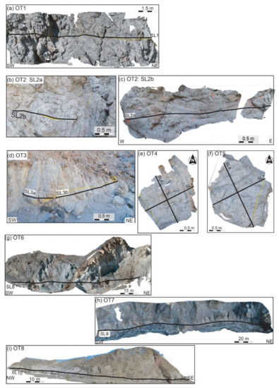
Figure 4.
Visualization of the eight outcrops studied in this work, including the scanlines (SL) location. (a) Outcrop 1 trending SW/NE shows heterogeneity of fracture orientation distribution. (b,c) Outcrop 2 trending E/W shows large NE/SW and NW/SE fracture planes crosscut by SL2a and SL2b. (d) Outcrop 3 trending NW/SE shows large E/W fracture planes crosscutting SL3a and SL3b. (e) Outcrop 4 consists in a fracture map; 2 scanlines were traced perpendicular to the main structures, recording then large E/W and N/S fracture planes for SL4 and SL5 respectively. (f) Outcrop 5 also consists in a fracture map; 2 scanlines were traced perpendicular to the main structures, crosscutting mainly fracture planes orientated NW/SE for SL6 and E/W for SL7. (g) Outcrop 6 consists in a canyon perpendicular to the SDVFZ segments, which crosscuts a large E/W fracture plane. This outcrop shows the transition between granitic basement and Crystal Spring sedimentary rocks. (h) Outcrop 7 trending NE/SW records a several fracture plane orientations. (i) Outcrop 8 trending NW/SE highlights mainly NE/SW and E/W fracture planes. SDVFZ: Southern Death Valley Fault Zone. For outcrops location, see Figure 2. Note that the OT6, 7 and 8 cross some major talus slopes. These outcrops have been modeled in 3D, making the fracture digitation possible to do in CloudCompare software. Then, the planes have been projected in 2D to keep data homogeneous from all fracture sets.
The fracture maps and the photogrammetric models were georeferenced and then used to extract the fractures in QGIS® software 2018, v.2.18.17. In this study, the fracture digitization was performed manually by tracing every detected fracture because of insufficient contrast between the fractures and the surrounding rock. Each digitized fracture became a georeferenced lineament in QGIS®. In the case of fracture maps, note that the fractures extending out of the sampling area were considered as one continuous feature [57,58,59] (Figure 2b). In QGIS®, the procedure of digitization consisted in an extraction of the end point coordinates of each fracture. Each fracture contained X and Y coordinates of each of the two end points, which helped to compute the spacings along a virtual scanline according to the following procedure:
- Digitized fractures are loaded in shapefile format (e.g., shp format);
- Virtual lines are traced along the georeferenced outcrop, and the intersection between the digitized fractures and the virtual line are collected. Note that, the intersection point ID must be the same as that of digitized fractures;
- X and Y coordinates are added to the intersection points file, computed directly in QGIS®;
- Values are classified according to X coordinate in Excel software, to ensure the right position of each intersected fracture;
- Spacings are computed following [17]:
||AB|| = √ (xb − xa)2 + (yb − ya)2
The calculated spacing in Equation (2) is not adjusted by Terzaghi correction. According to the scanline orientation, fracture orientations, and the position of scanline intersections for each fracture set, the fractures spacing were adjusted by applying the Terzaghi correction following [60]:
S = SA × cos θ
S is the true mean spacing of fractures in a set, SA is the apparent mean spacing of fractures in a set and θ is the acute angle between the direction normal to fractures and the scanline.
Orientation bias can be minimized by drawing a scanline parallel to the normal to a fracture set, such that θ is close to 0°. All fractures intersected by scanlines were acquired. Then, all measured fractures were filtered by orientations during the analysis in order to describe the patterns of spacing according to each fracture set.
3.2. Fracture Orientation Analysis
In this study, the orientation is the first parameter analyzed to classify the fractures into fracture sets. As described before, from virtual scanlines, the fracture dip was not obtained from virtual scanlines, while it was measured for each fracture on field scanlines. The fracture dip has been measured for each fracture. Here, the classification into fracture sets is based only on strike orientation without considering the variation in dip to preserve data homogeneity. Note that, from field scanlines, the dip direction for each fracture is however provided in the Schmidt canvas.
Several software packages such as Win-tensor [61], Stereonet [62], and Digifrac [63] have been developed in order to project the structural data. Fisher distribution [64], Fisher-Bingham distribution [65], and von Mises distribution [66] are commonly used to describe symmetrical distributions of orientations in 2D, and sometimes in 3D in case of Fisher distribution. However, these distributions do not describe complex asymmetrical data. Then, the classification was performed using the mixture of von Mises distribution (MvM) [67], which is adapted to describe complex circular data and then seem relevant to model larger complex fracture networks. The methodology consists in a semi-automated approach based on appraisal tests to avoid any subjectivity in fracture set analysis. This distribution is based on three parameters: (1) Mean orientation (µ°), around which the distribution is centered; (2) kappa (κ), which controls the concentration of the orientation values around the mean; and (3) weight (ω), corresponding to the relative contribution of each fracture set to the model. In addition, the best number of fracture sets is approved using the goodness of fit parameters (e.g., likelihood). The degree of precision of each mean fracture orientation is computed using the standard deviation (SD), which is of +/−10°. For further explanations, see Chabani et al., [68], which described and adapted the MvM methodology for structural data. To plot the orientation data in the current study, we used a rose diagram for describing data which only contain dip direction measurements, and Schmidt canvas for describing data which contain strike and dip measurements.
3.3. Analysis of Spacing
Numerous statistical tools have been developed in the recent decades specially to analyze the facture parameters such as spacing, width, length, orientation [26,51,52,53], and its spatial distribution (e.g., clustered, random, or uniform distribution) [26]. For spacing parameter, a coefficient of variability (Cv) has been widely described in the literature, that provides an indication of the fracture distribution [20,26,54,69]. It is given as:
Cv = σs/S
σs and S represent, respectively, the standard deviation and the mean spacing. When Cv ≈ 1, the fractures intersected by the scanline are distributed randomly. When Cv < 1, fractures are more regularly spaced, while Cv = 0 represents uniformly spaced fractures, and Cv > 1 indicates fractures that are more irregularly spaced. Each Cv value can provide information about the degree of fracture clustering [26].
The heterogeneity of fracture distribution based on cumulative distribution has also been quantified using the V′ statistic of [70], applied to structural geology by [20,30,31]. Indeed, the heterogeneity of distribution of the fractures and associated parameters (aperture, spacing, thickness, etc.) may be characterized from the cumulative frequency using the method described by [70]. Then, V′ is defined as the measure of the heterogeneity within the scanline, which is given as:
V′ = |Dmax| + |Dmin|/A
Dmax and Dmin are the cumulative frequency at that point if the fracture parameter was uniformly distributed [30]. Dmax and Dmin are positive and negative respectively. A is the total cumulative frequency of the analyzed parameter. In the present study, the V′ will be used on aperture parameter in order to evaluate the strain heterogeneity. This strain heterogeneity depends on the amount of displacement (aperture or heave) and the spatial distribution of the fractures [31]. Analogical tests have been illustrated by Putz-Perrier and Sanderson [31] for two examples of the same population of extensional fractures, with different spatial arrangement, but with same strain. They obtained a fracture network uniformly distributed for the first example, and strongly clustered for the second one. Then, aperture parameter helps us to better characterize the degree of heterogeneity of every analyzed area. A perfect regular fracture distribution produces a V′ ≈ 0 as fracture sizes decrease, while the maximum heterogeneity of fractures distribution would produce a V′ = 1 value. For further explanations, see Putz-Perrier and Sanderson [31].
3.4. Fracture Density P10
The position and spacing of a set of fractures are considered whatever of their type (e.g., normal, reverse, etc.) [20]. A scanline normal to a set of fractures would intersect N fractures (number of fractures) over a length. The fracture density (P10) is defined as the number of fracture intersections (N) per unit length (L) [58], following:
P10 = N/L
3.5. Cumulative Frequency Diagrams
The spacing distribution and arrangement were analyzed by using cumulative frequency. As recommended by [20,26], stick plots were used, in which the location of each fracture intersected by the scanline is mentioned. This allows to better visualize the fracture distribution. Furthermore, a plot of cumulative frequency versus distance along the scanline (from the beginning to the end) was used, in which P10 is proportional to the slope of the cumulative curve. The cumulative plot is normed by the maximum value, expressed in percentage (%) and it always starts at the origin (0, 0) and ends at (dN − d1), (N − 1). The parameters d1 and dN represents respectively the first and the last fracture. The cumulative frequency (%) against distance along the scanline provides a rapid visual comparison between datasets for each scanline and between those scanlines whatever their lengths [71].
4. Results
4.1. Description of Fracture Systems Acquired from NH Range
The studied outcrops reported in the Figure 2 were distributed homogenously within the entire central part of the NH (CBS). The structural position of each outcrop is described below.
4.1.1. Fieldwork Scanlines
The fracture network parameters were compiled from the field (Figure 2). The measurements were performed within OT1 using a scanline 1 (SL1 orientated N010) of 13.45 m length (Figure 4a), intersecting a total of 324 fractures, with a mean space of 0.04 m (Table 1). The orientation, spacing and aperture data were acquired along two scanlines with different orientations in OT2 (Figure 4b,c). The SL2a (orientated N160) of 7.5 m length intersected 109 fractures, with a mean space of 0.07 m, while the SL2b (orientated N070) of 1.64 m length intersected 37 fractures, with a mean space of 0.04 m. Within OT3, the fracture spacing and aperture were also acquired along two different orientation scanlines: SL3a and SL3b orientated N055 and N160 respectively (Figure 4d). Both scanlines intersected respectively 31 and 47 fractures, with a mean space of 0.03 and 0.06 m.

Table 1.
Characteristics of the fractures acquired from each studied outcrop, along the scanlines. Outcrop 1 to 3 (without asterisk) show the characteristics of the fractures acquired directly from field scanlines. Outcrop 4 to 8 (with asterisk) show the data extracted from aligned photographs using Metashape Software v.1.6.5, with a virtual scanline. For each outcrop, number of scanlines are indicated with: Number of fractures intersected, orientation and length of scanlines, mean fractures space, density (frac/m), coefficient of variability (Cv), and V′ statistic fom [70]. The proximity to the major faults is mentioned. Mean spacing and Cv are computed with Terzaghi correction. Sgmt: segments.
4.1.2. Virtual Scanlines
The fracture variability analysis was further conducted by creating, fracture maps with a resolution of 2 × 10⁻⁴ m, OT4 and OT5. OT4 is sized 1.7 m per 1.6 m and is located in the granitic facies close to the SDVFZ segments (Figure 4e). Two scanlines: SL4 and SL5, orientated, respectively, N163 and N073, were traced perpendicular to each other in order to intersect the maximum number of fractures and avoid angular bias (e.g., [26]). In total, 28 fractures were intersected along SL4 of 0.80 m length, with a mean space of 0.02 m. Regarding the SL5, 46 fractures were intersected, with a mean space of 0.04 m (Table 1). OT5 is sized 1.8 per 1.7 m and is also located in the granitic facies, close to the SDVFZ segments (Figure 4f). Here again, two scanlines: SL6 and SL7 were traced, orientated respectively N074 and N157. They intersected, respectively, 26 and 31 fractures. The mean spacing is of 0.05 and 0.02 m for SL6 and SL7, respectively.
To perform the fracture variability study in 1D, three photogrammetric models localized only in the granitic facies were added to the present work. They are located close to the major fault segments. The fractures extracted from these models ranged from 10−2 to 20 m in length.
The drone photogrammetric model displayed in OT6 is sized approximately 110 per 45 m (Figure 4g); 171 fractures were traced and are intersected by the SL8. Note that OT6 presents various lithologies including granitic rocks, gneiss, gabbro, and sedimentary rocks. This may influence the spatial variability of the fractures in this area, as it will be discussed below. The drone photogrammetric model presented in OT7 is sized approximately 82 per 45 m. In this model, 188 fractures were traced and intersected by the SL9 (Figure 4h). Finally, drone photogrammetric model displayed in OT8 is sized approximatively 100 per 25 m. In total, 258 fractures were traced and intersected by SL10 (Figure 4i).
4.2. Fracture Orientation Distributions
The data acquired from scanlines in the central part of the NH show a heterogenous fracture distribution. SL1 is located near (around 10 m) a SDVFZ major segment (bold black line in Figure 2b), which acts following dextral strike-slip movement. Several lineaments are identified from the high-resolution field mapping, striking E/W (GFZ signature) to NW/SE (SDVFZ signature). From the SL1, the mean fracture orientations (µ) are striking N026, N062, N092, N130, and N171 (Figure 5a, Table 2). Fracture abundances for each fracture set are characterized by a slight dominance of the N062 and N092 fracture set with, respectively, 21% and 37% (Table 2). N026, N130, and N171 fracture sets represent, respectively, 17%, 15%, and 10% of the whole fracture set. Then, NE/SW trend appears at outcrop scale and is equivalent to E/W fractures in term of density. However, SL2a crosscut by SDVFZ major segment and close to thrust fault (Figure 2b), and a significant difference was observed in terms of fracture abundance with respectively 80 fractures in comparison with SL1 (261 fractures). The most recorded fracture sets are striking N014, N025, and N102 with, respectively, 18%, 46%, and 27%. The other fracture sets do not exceed 10% (Figure 5b, Table 2). N152 is the most dominant fracture orientation highlighted along the SL2b, representing 38%. N003 and N112 both represent 31% (Figure 5c, Table 2). Both SL3 scanlines are located far from the influence of the SDVFZ segments, thrust faults and sinistral strike-slip faults (Figure 2b). Then, SL3a, much smaller in length, intersected three fracture sets: N077, N098, and N135 with, respectively, 49%, 25%, and 26% abundances (Figure 5d, Table 2). Three fracture sets were also highlighted from the SL3b striking N040 (24%), N081 (65%), and N150 (11%). The orientations of fractures detected in SL3 scanlines are less heterogenous than in SL2 and SL1. The structural position of SL3 far from major faults (around 40 m in distance) very likely impacts the fracturing at outcrop scale.

Figure 5.
Fracture orientation distributions of the NH studied outcrops (a–l). (a–e) The fracture orientation distributions are represented into Schmidt canvas, lower hemisphere because they contain strike and dip measurements. (f–l) Fracture orientation distributions are represented by rose diagrams because they contain only dip direction measurements. Each direction rose diagram of direction is expressed with classes of 5°. The dashed lines indicate the direction of the scanline. n: Number of data. See legend in the figure for colors.
Table 2.
Output parameters obtained from the MvM distribution fitting to fracture orientation data. Each scanline dataset was analyzed separately. Each simulation provides the number of fracture sets with their corresponding mean orientation µ (°), kappa (κ) which corresponds to the orientation variance around the mean, and weight (ω) corresponding to the proportion of each fracture set. Cv: Coefficient of variability.
Regarding the virtual scanlines, the structural position of SL4 (OT4 orientated N163) and SL5 (orientated N073) is the same as SL1. Indeed, both scanlines are located near SDVFZ major segment (around 6 and 4 m in distance, respectively), highlighted by dominance of NW/SE and E/W structures. SL4 intersected much less fractures in comparison with the perpendicular SL5 (Table 1). SL4 displayed three fracture sets striking N034 (34%) and N086 (53%), and N123 (13%), while SL5 highlighted five fracture sets striking: N001 (39%), N018 (12%), N040 (14%), N113 (9%), and N144 (26%) (Figure 5f,g, Table 2). SL6 and SL7 orientated, respectively, N074 and N157, acquired from OT5, showed a heterogeneous fracture set, and are located near SDVFZ segments (4 m distance). Indeed, SL6 highlighted three fracture sets striking N004, N100, N161 with, respectively, 35%, 49%, and 16%, while SL7 highlighted N053, N087, and N116 fracture sets with, respectively, 13%, 81%, and 6% (Figure 5h,i, Table 2).
Crosscutting the NW/SE thrust faults (in red lines, Figure 2b) and SDVFZ segment faults (in black bold lines, Figure 2b), the OT6 to OT8 displayed heterogeneous fracture orientation distribution from scanline measurements. SL8 scanline acquired within OT6 is characterized by a special geological setting. Indeed, compressional structures like thrust faults crosscut this outcrop (Figure 2b), close to the Canadian Club Wash (Figure 1c). SL7 is however crosscut by 2 SDVFZ major segments. Regarding the orientation distributions, SL8 of 109 m length, orientated N020, recorded three fracture sets, striking N058, N090, and N132 with an equivalent fracture abundance (between 32% and 36%) (Figure 5j, Table 2). However, five fracture sets were highlighted from SL9, striking N029 (20%), N060 (27%), N096 (9%), N132 (22%), and N176 (22%) (Figure 5k,l). SL10 recorded N004 (3%), N040 (7%), N091 (73%), and N118 (17%) fracture sets. This scanline crosscut a thrust fault and several secondary SDVFZ segments (Figure 2b).
4.3. Spatial Distribution of Fractures
The spatial organization of fractures was highlighted from scanlines, whatever the fracture orientation, and is summarized in Table 1. In addition, the spatial organization was also studied following the fracture orientations in order to determine the impact of some regional directions on the NH structural organization.
From SL1, fracture density (P10) and Cv are around, respectively, 19.4 frac/m and 1.2, indicating a random fracture distribution. Equivalent P10 and Cv were measured from SL2b with, respectively, 19.5 frac/m and 1.1, also indicating a random distribution. While SL2a recorded a P10 of 10.6 frac/m and Cv of 14.4, indicating a less abundant and highly clustered fracture system. Values of P10 of 31.8 and of 8.4 frac/m, Cv of 0.7 and 1.7 were highlighted from SL3a and SL3b, respectively, (Table 1), indicating very abundant fractures with a random distribution.
Three different spacing organizations were identified from fracture sets in SL1 (Table 2):
- Fractures distributed randomly in fracture set N026 with Cv = 1.03;
- Fractures uniformly spaced in fracture set N062 with Cv = 0.53;
- Fractures more irregularly spaced or clustered in fracture sets N092, N0130, and N171 with, respectively, Cv = 1.44, 1.43, and 1.37.
The fracture distribution presented in Figure 6 shows the layout of fractures and their location along each scanline. For SL1, the fracture distribution is showed using a cumulative frequency plot against the position of fractures along the scanline for each fracture set (Figure 6a). Two major trends are distinguished: (1) Regular fracture distribution from the beginning to the end of the scanline especially for fracture sets N026 and N171 (respectively in black and orange colors with diamond and square symbols in Figure 6a); and (2) a regular fracture distribution at the beginning, then clustered (increased frequency), followed by another regular distribution at the end for fracture sets N062, N092, and N130 (respectively in red, green and purple colors in Figure 6a). Three fracture clusters having a slope higher than 2 are highlighted in N062 fracture set, around 5.5, 8, and 10 m (Figure 6a), highlighting a clustered spacing. Note that, this slope corresponds to the shape of the cumulative frequency compared to the uniform distribution highlighted in the plots below (Figure 6). The cumulative frequency plot highlighted one fracture cluster around 12–13 m in the N092 fracture set. Within the N130 fracture set, two fracture clusters are characterized around 3–4 and 10 m.
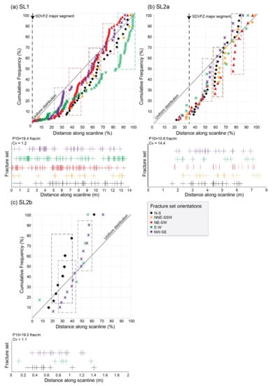
Figure 6.
Cumulative frequency diagram along each scanline and following each fracture set (in colors). Plot of cumulative frequency expressed in % versus distance along scanline for: (a) SL1, (b) SL2a, and (c) SL2b. Dashed lines indicate a potential cluster for each fracture distribution, indicating a rapid increase in the number of fractures with slope threshold > 2. The diagonal line in each plot of cumulative frequency defines a uniform or regular distribution. Visual location of fractures expressed in stick plots for each fracture set distribution, highlighting the fracture position along the scanline, including the fracture density (P10) and the coefficient of variation (Cv) values. The structural position is done in each diagram. See the color legend for the orientation of fracture sets.
SL1 is in moderate deformation zone, affected mainly by SDVFZ major segment and some E/W fault segments. The position of SL1 close to SDVFZ major segment, trending NW/SE creates these irregularities in fracture distribution. Indeed, the NW/SE (N130) fracture set is one of the most clustered fracture sets. The intermediate (in term of length) E/W segments shown in the Figure 2b have a strong impact on N092 fracture set distribution, making it the more clustered distribution with Cv = 1.44.
A high fracture density is observed in the central part of the SL2a profile (Figure 6b). Indeed, five fracture clusters were identified in which the fracture density is increased around 3–4 m in N143 fracture set (purple color in Figure 6b), 4.5 m in N014 and N025 fracture sets (black and orange colors, respectively, for N014 and N025 in Figure 6b), and around 6 m in N014 and N050 fracture sets, displayed, respectively, in black and red colors for N014 and N050 in Figure 6b. The SDVFZ crosscuts the SL2a profile and introduces some irregularities in fracture distribution since the beginning, mainly in N143 and N014 fracture sets, highlighting then an anisotropy following some directions.
Fractures intersected by the SL2b are distributed randomly whatever the direction with Cv close to 1 (Table 2). N098 and N0135 fracture sets intersected by SL3a displayed a Cv of 0.6 and 0.8, indicating a uniform spacing organization, while Cv of 1.07 measured from the N077 fracture set indicates a clustered organization. However, the beginning and the end of the SL2a profile showed a regular fracture distribution. Along SL2b, a random fracture distribution was observed whatever the fracture orientation with Cv around 1 (Figure 6c). Three fracture clusters are, however, detected within N003, N112, and N152 fracture sets (displayed respectively in black, green, and purple colors), respectively, around 0.4–0.6, 0.8–1, and 1.2 m (Figure 6c).
A regular fracture distribution was highlighted within fracture orientations N098 and N135 along SL3a profile, with Cv of 0.6 and 0.8, respectively (Figure 7a). For N077 fracture set (red color with triangle symbol), a clustered distribution was shown with two fracture clusters around 0.3–0.4 and 0.7–0.8 m. However, along SL3b scanline profile, one fracture cluster which corresponds to an increase in fracture density was shown around 2 and 2.25 m, respectively, in N040 and N150 fracture sets (respectively in red and purple colors in Figure 7b). Only three fracture clusters were identified around 1.5, 2.5–3, and 4 m in N081 fracture set (green color). A regular fracture distribution was characterized outside these fracture clusters. Located away from major fault segments, around 40 m distance, the SL3a and SL3b profiles displayed a very poor fracture system organization and fracture density. In addition, these profiles are in a moderate deformation zone, which can impact drastically the fracture distribution and density. Boudinage structures and brittle shearing are not observed within this area.
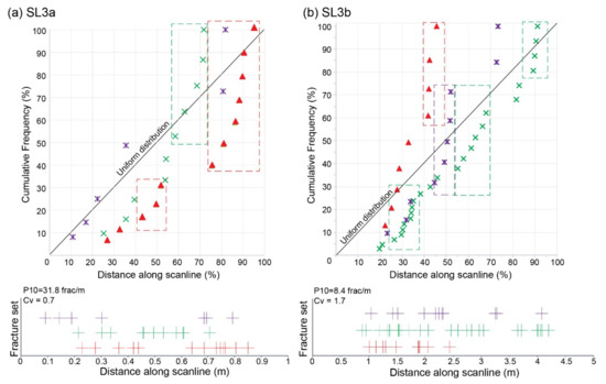
Figure 7.
Cumulative frequency diagram along each scanline and following each fracture set (in colors). Plot of cumulative frequency expressed in % versus distance along scanline for: (a) SL3, and (b) SL3a. Dashed lines indicate a potential cluster for each fracture distribution, indicating a rapid increase in the number of fractures with slope threshold > 2. The diagonal line in each plot of cumulative frequency defines a uniform or regular distribution. Visual location of fractures expressed in stick plots for each fracture set distribution, highlighting the fracture position along the scanline, including the fracture density (P10) and the coefficient of variation (Cv) values. See the color legend in Figure 6.
OT4 and OT5 are in a moderate deformation zone, affected mainly by SDVFZ major segment and some E/W fault segments. From virtual scanlines, three fracture sets were recorded in SL4. The N034 fracture set highlighted one fracture cluster around 0.5–0.6 m (red rectangle in Figure 8a). However, four fracture clusters were highlighted at the beginning and at the end of the SL4 profile within N086 fracture set (green color with cross mark symbol in Figure 8a), around 0.01, 0.25, 0.65, and 0.7–0.8 m. The rest of the intervals are characterized by a regular fracture distribution. The SL5 scanline recorded five fracture sets and are characterized by a regular fracture distribution whatever the fracture set (Figure 8b). An increased fracture density is identified within the N001 fracture set (black color) around 0.7 and 1.2 m.
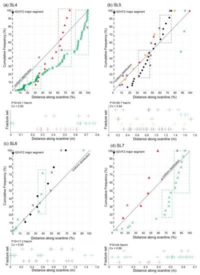
Figure 8.
Cumulative frequency diagram along each scanline and following each fracture set (in colors). Plot of cumulative frequency expressed in % versus distance along scanline for: (a) SL4, (b) SL5, (c) SL6, and (d) SL6. Dashed lines indicate a potential cluster for each fracture distribution, indicating a rapid increase in the number of fractures with slope threshold > 2. The diagonal line in each plot of cumulative frequency defines a uniform or regular distribution. Visual location of fractures expressed in stick plots for each fracture set distribution, indicating the fracture position along the scanline, including the fracture density (P10) and the coefficient of variation (Cv) values. The structural position is done in each diagram. See the color legend in Figure 6.
Fractures detected within SL6 are mainly distributed regularly for N004 and N161 fracture sets (displayed respectively in black and purple colors in Figure 8c), with Cv of 0.88 and 0.84, respectively. Cv of 1.35 was, however, computed from the N090 fracture orientation (green color with cross mark symbol, Figure 8c), indicating highly clustered fractures. Then, one fracture cluster was identified around 0.5–0.6 m (Figure 8c). The three fracture sets striking N053, N087, and N132 are recorded mainly with fractures regularly distributed along the SL7, with Cv ranging from 0.83 to 0.84 (Figure 8d). Two fracture clusters are then identified within the N087 fracture set (green color with cross mark symbol in Figure 8d) around 0.5 and 0.6–0.7 m.
The influence of the regional directions was observed on E/W fractures orientation, with a higher density and clustering within this fracture set (Table 2). However, the NW/SE direction is less expressed in comparison with SL1 and SL2. The small length of OT4 and OT5 scanlines may influence the result and then introduce some bias to the analysis.
Near the Canadian wash (see Figure 1c for location), OT6 is located close to the highly deformed zone (for location, see Figure 2). Two major faults crosscut this outcrop: SDVFZ major fault segment and thrust fault. SL8 intersected three fracture sets with a high fracture density interval (Figure 9a). Three fracture clusters were identified in N058 fracture sets, respectively, around 10–20, 40, and 75 m (red color with triangle symbol legend, Figure 9a). The fracture clusters in N090 fracture set (green color with cross mark symbol, Figure 9a) are around 40, 50–60, 75, and 80 m. Finally, within N132 fracture set (purple color with strikethrough cross, Figure 9a), two fracture clusters comprised between 10–15 and 50–70 m were identified. We are fully aware that the canyon presents a complex structuration due to various lithologies and the overprinting faults.
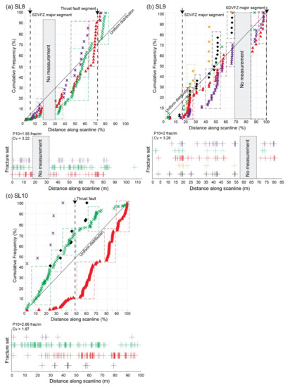
Figure 9.
Cumulative frequency diagram along each scanline and following each fracture set (in colors). Plot of cumulative frequency expressed in % versus distance along scanline for: (a) SL8, (b) SL9, and (c) SL10. Dashed lines indicate a potential cluster for each fracture distribution, indicating a rapid increase in the number of fractures with slope threshold > 2. The diagonal line in each plot of cumulative frequency defines a uniform or regular distribution. Visual location of fractures expressed in stick plots for each fracture set distribution, showing the fracture position along the scanline, including the fracture density (P10) and the coefficient of variation (Cv) values. See the color legend in Figure 6.
Additionally located in the highly deformed zone, SL9 is crosscut by two SDVFZ major segments. Several fracture clusters are observed as following (Figure 9b):
- N029 fracture set with one fracture cluster identified around 20 m;
- N060 fracture set with four fracture clusters characterized around 20, 42, 47, and 80 m;
- N096 fracture set with one fracture cluster identified around 15–20 m;
- N132 fracture set with five fracture clusters identified around 15–20, 35, 40–45, 55, and 80 m;
- N176 fracture set with four fracture clusters identified around 20, 25, 35–40, and 55 m.
SL10 scanline crosscuts several secondary SDVFZ segments and a thrust fault, in moderate deformation domain. A regular distribution of fractures was encountered in N004 fracture set (black color with diamond symbol legend in Figure 9c). Three fracture clusters were detected around 30–40, 55–65, and 80–90 m in N040 fracture set (data in red with triangle symbol legend, Figure 9c), while in N091 fracture set, the fracture clusters are around 10–20, 28, 40, 60–70, and 90 m (green color with cross mark symbol, Figure 9c). The E/W and NE/SW fractures orientations are more expressed in terms of fracture density which can be enhanced by the position of the major faults in this area.
4.4. Fracture Aperture Distribution
The heterogeneity of the fractures distribution and associated parameters (e.g., aperture, spacing, etc.) can be determined using the Kuiper’s method [20,30,31,70]. In this study, the V′ is used to better precise the degree of heterogeneity of aperture distribution along scanlines. V′ values are summarized in Table 1 for only data acquired from the fieldwork. Confidence interval of 95% was used to compile V′. Then, a cumulative aperture was plotted against fracture location along the scanline (Figure 10). Application of the Kuiper test shows V′ = 0.29 for SL1, meaning that the apertures are distributed randomly (Figure 10a). For SL2a and SL2b, V′ is, respectively, 0.42 and 0.50 despite the difference in term of scanline length and orientation (Table 1, Figure 10b,c). These values indicate that the apertures are distributed randomly along each scanline. The same result of aperture distribution is shown along the SL3a and SL3b (Figure 10d,e), with V′ of 0.32 and 0.57, respectively. The fracture aperture distribution is more heterogeneous in SL3b and SL2b, than in SL1, SL2a, and SL3a.
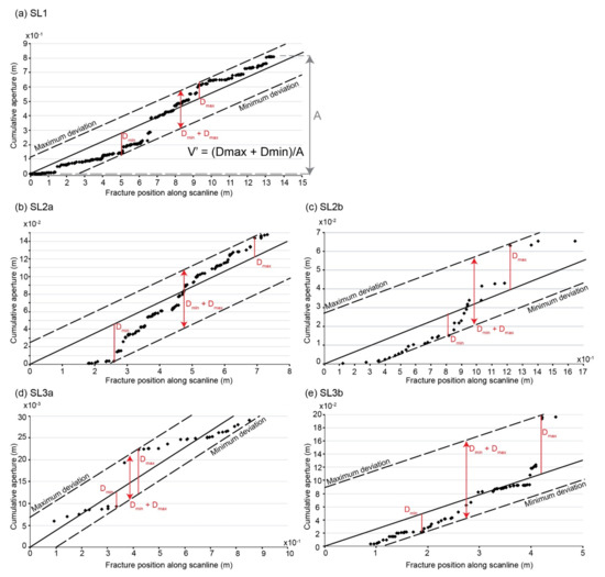
Figure 10.
Plot of the sum of all apertures (cumulative fracture aperture) intersected along a scanline to show V′ for (a) SL1, (b) SL2a, (c) SL2b, (d) SL3a, and (e) SL3b. The diagonal of each plot (black line) represents the uniform distribution linking the origin to the cumulative aperture to the end of the scanline (for further explanations, see [20,30]). Dmax and Dmin correspond to the maximum and minimum difference between the cumulative aperture and the uniform strain line, respectively. V′ quantifies the heterogeneity of the strain distribution, varying from 0 (uniform distribution) to 1 (maximum possible hetrogeneity).
The possibility of any correlation between the fracture orientation and the aperture was tested using a plot of aperture against fracture set for each scanline (Figure 11). The mean fracture aperture in SL1 is about 2.5 mm and, therefore, lower than in fractures of SL2a and SL2b at, respectively, 2 and 1.7 mm. In SL1, the widest fracture apertures are around 10 mm, and occurred in fractures orientated N092 (Figure 11a). The most common observed fractures in the field were affected by mineralization of carbonates mostly (Figure 12). The widest fracture apertures detected in fracture orientation N092 are classified as fully sealed by carbonates (Figure 12a). In SL2a, the maximum fracture aperture is also 10 mm and belongs to the N050, N150, and N170 striking sets (Figure 11b). The widest fracture apertures are classified as fully sealed by carbonates and oxides (Figure 12a,b). In SL2b, the maximum fracture aperture does not exceed 8 mm, and occurred in fractures striking N009 and N090 (Figure 11c) and classified as fully sealed by carbonates and oxides.
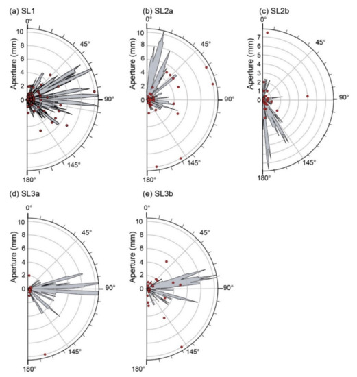
Figure 11.
Half circular diagram showing the relation between fracture strike and apertures. (a) SL1, (b) SL2a, (c) SL2b, (d) SL3a, and (e) SL3b. Apertures from SL4 to SL10 are not available. Rose diagram scaled for mean aperture with classes of 5°.
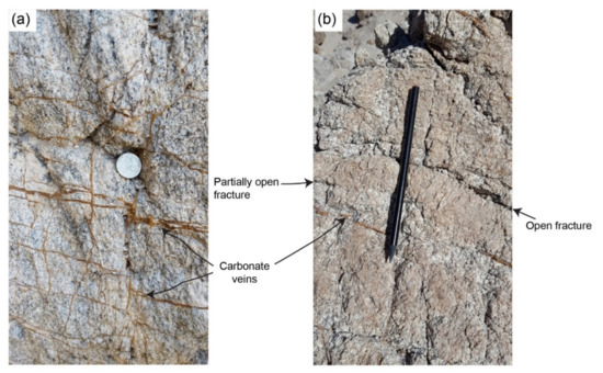
Figure 12.
Illustration of the observed fractures observed in the field, mostly affected by mineralization. (a) Picture taken near OT6 illustrating veins fully sealed by carbonates. (b) Picture taken near the Canadian Wash illustrating open and partially open fractures. The carbonates are ubiquitous following SDVFZ trend (i.e., NW/SE). The fractures striking E/W have been observed with a wider aperture and were filled by barite and oxides.
The mean fracture aperture in SL3a and SL3b is about 0.9 and 2.8 mm, respectively. The maximum fracture apertures are around 10 mm. They occur in fractures striking N162 and N150 for SL3a and SL3b, respectively (Figure 11d,e). The maximum fracture apertures identified in SL3a occurred in fractures classified as partially open (Figure 12b), while in SL3b, the maximum fracture apertures occurred in fractures classified as fully sealed by carbonates and oxides. The fracture aperture distribution are more heterogenous in SL3b than in SL3a, in which apertures are generally lower than 2 mm.
As a summary, the distribution of the apertures in the central part of NH is ruled by a random behavior. Regarding the relationship between apertures and the orientations, an anisotropy was observed following E/W trend, which presents fractures with a wider aperture.
5. Discussion
5.1. Representativness of the Fieldwork and Virtual Scanlines
The present study covers a sampled fracture network from fieldwork and virtual scanlines obtained from photogrammetry. The moderate linear density compiled from the virtual scanlines, especially in SL8, SL9, and SL10, does not exceed 3 frac/m. The highest linear density is detected in SL4 and SL7 with, respectively, 42.1 and 44 frac/m. From fieldwork scanlines, the linear densities ranged between 8.4 frac/m in SL3b and 31.8 frac/m in SL3a.
Regarding the sampling resolution, in case of virtual scanlines, the shorter fracture measurement is around the decimeter to meter and depends on the photogrammetric image resolution, while in the case of fieldwork scanlines, the measurement resolution is around the millimeter. The difference in resolution strongly impacts the fracture density and its representativeness. The low density of the fractures detected from virtual scanlines might not be fully considered as representative of the whole granitic rock. However, it is very useful in zones with difficult access.
In the case of sampling in 1D, a scanline perpendicular to the fractures will detect a maximum of sub-set of all fractures. Then, the probability that a fracture is detected within a scanline is proportional to the fracture surface area [72]. In basement rocks, fractures that span the sampling study area limits whatever its lengths and heights will reflect 3D sampling. The same case is observed in sedimentary rocks when fractures span the layers and the limits of the studied area [72].
5.2. Consistency of the Recorded Fracture Sets
The main dominant orientations recorded from the different scanlines displayed in the central part of the NH highlight the fact that NH geometry is controlled by NE/SW, E/W, and NW/SE trends (Figure 13). From fieldwork scanlines, the E/W and NW/SE fracture sets are the most consistent orientations whatever the scanline. The N/S, NNE/SSW, and NE/SW fracture sets are only recorded in the SL1 and SL2a fieldwork scanlines (Figure 13). SL2b, SL3a, and SL3b detected mostly E/W and NW/SE directions with a heterogeneous recording (Figure 13). The E/W is the most dominant trend within SL3b, while the NW/SE trend dominates within SL2b, and constitutes the second and third dominant fracture sets within SL3a and SL3b, respectively. The variability in fracture orientation may be related to the influence of the major faults. Indeed, as showed in Figure 2, the position of SL1 and SL2a close to the SDVFZ segment interfering with the thrust fault induces an additional complexity in the structural signature. As mentioned before, a clear overprinting has been recognized between primary SDVFZ and syn-kinematic dextral strike slip faults related to the transcurrent movements followed in time by compressive structures. Thrusting is postdating the activity of the SDVFZ, and it is tempting to relate the thrust structures to activity along the frontal termination of GFZ which acts with a sinistral strike slip movement.

Figure 13.
Plot displaying the mean orientation with arrows of each collected fracture set from NH scanlines. Each arrow was characterized by its own length, which corresponds to the fracture set abundance. The horizontal line above each arrow corresponds to the standard deviation of each fracture set, using an interval of confidence of 75% (see [68] for more explanations). Each color arrow corresponds to a fracture set. Orange arrow: NNE/SSW fracture set, red arrow: NE/SW fracture set, green arrow: E/W fracture set, yellow arrow: NNW/SSE fracture set, purple arrow: NW/SE fracture set, and black arrow: N/S fracture set.
In the southern end of the NH central area, E/W trending structures showing evidences of compression again possibly related to GFZ activity are even clearer.
Regarding the fracture orientations highlighted from the virtual scanlines, a reproducible and consistent NE/SW, E/W, and NW/SE fracture sets are encountered (Figure 13). The GFZ is confirmed as a major fault which influences the NH geometry and induces the E/W fractures which are more expressed in SL4, SL6, SL7, SL8, and SL10. According to Chabani et al. [25], who describe the spatial organization of a NH fracture network at different scales from 2D maps and previous works [47,48,49,73], the compression episode at the southeastern end of the NH and at the front of the Avawatz mountains plays a key role in the increase of the fracture intensity in the central domain of NH, and can explain the consistency of the E/W direction in the whole internal NH domain.
The NW/SE direction is the second most reproducible direction recorded along the internal part of NH (Figure 13), related to SDVFZ activity, which acts with a dextral movement. This direction is more expressed especially near the Canadian wash, where the deformation is important, following a second order scale as described by Chabani et al. [25].
The N/S and NE/SW fracture sets are also highlighted from the virtual scanlines but are less consistent than the E/W and NW/SE directions. These directions are heterogeneous with more than 25° (dispersion of the mean orientation) of variability in case of the NE/SW fracture set (Figure 13). These trends are highly dependent on the scale of observation and have no influence on the NH geometry [25].
As mentioned before, a recent study by Chabani et al., [25] revealed the same influence of the E/W and NW/SE fracture sets in the central part of NH. Indeed, E/W and NW/SE trends control the NH geometry within the third and fourth order scale. In addition, the major faults played a key role in the fracture density increase following different areas inside the central part of NH. The gradient of deformation shown in Klee et al. [34] and Chabani et al. [25] induced fracturing notably near OT6 and OT7, in which the strain gradient is the highest.
5.3. Clustering of Fractures in Central Part of NH
Figure 14a highlighted the Cv for the relative spaces between adjacent fractures for each studied scanline, by plotting the values against the overall fracture intensity. This correlation helps to better compare the Cv values and assess the spatial organization of the fractures. A large range of behaviors were observed. A regular spacing distribution (Cv < 1) was highlighted especially from SL3a, SL4, SL5, SL6, and SL7 (Figure 14a, Table 1). However, a more clustered distributions (Cv > 1) was observed in the SL1, SL2a, SL2b, SL8, SL9, and SL10. This large variation is probably related to the prominent influence of the thrust faults and the SDVFZ major segments close to SL8, SL9, and SL10, and only the influence of the SDVFZ major segments in the case of SL1 and SL2 profiles. However, the location in moderate deformation zone and away from major faults of SL3 scanlines highlight the absence of any organization in the fracture systems. They confirm the key role of the structural heritage (regional directions) in fracture patterns at outcrop scale. Recent study by Franklin et al. [74] highlighted and confirmed that the clustered spacing distribution is pronounced at the outcrop scale and is related to the influence of the major faulting.
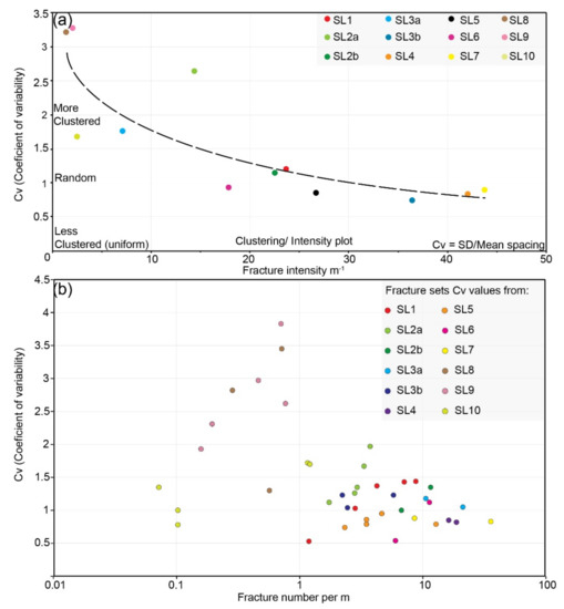
Figure 14.
(a) Coefficient of variability (Cv) plotted against fracture intensity (P10) of the NH studied outcrops. SD: Standard of deviation of spacing measured from each scanline; mean: Mean spacing measured from each scanline. (b) Coefficient of variability (Cv) plotted against fracture number normalized by the scanline length.
From all the analyzed datasets, note that the outcrops with the greatest numbers of fractures are most usually characterized by random patterns. This observed relationship could be interpreted as the result of the increasing spatial heterogeneity of the fracture pattern with increasing strain. In that case, OT6 to OT8 highlighted that the greatest number of fractures, the fracture density, and the strong clustering within fracture sets can be related to the intensity of deformation in this area and the proximity to the SDVFZ major segments and thrust faults. Indeed, the new geological map displayed in Figure 2b highlighted a stacking of the Crystal Spring series, intruded by the Mesozoic granite. In addition, the thickness of Crystal Spring series was reduced, as they were dragged, and stretched laterally against the granite due to the SDVFZ activity, especially in OT6 to OT8 areas. This intense deformation affected the entire NH range with local evidences of extreme shearing. However, we are aware that the presence of several different lithologies with varying competences within OT6 may bias the fracture distribution and its interpretation. In addition, the structural architecture of this area is the most complex within NH range as it includes overprinting deformation phases. A future publication dedicated to these overprinting issues is in preparation.
Another approach approved by Hooker et al. [30] consists of cross-examining the low number N of datasets. Cv values are commonly indistinguishable from random for low-N sets. Then, Cv increases with increasing fracture abundance (Figure 14b). This observation reflects an increase in fracture clustering with fracture abundance only in case of fracture sets detected from virtual scanlines (SL8, SL9, and SL10, Figure 14b). In case of fractures detected from fieldwork scanlines, the trend is more unclear since the Cv evolution is still comprised between 0.5 and 1.5, whatever the fracture abundance (Figure 14b). Once again, the proximity to major faults in case of SL8, SL9, and SL10 may play a key role in the fracture patterns growth. For SL1 to SL7, the fracture organization may be perturbed by the abundance of the E/W facture orientation, which can increase drastically the fracture abundance following E/W fracture set trend. This may be related to the scanline orientation which cannot intersect the rest of the fracture sets. From SL1 to SL7, fracture set trending E/W is more expressed than the rest of the sets except for SL2a, SL2b, and SL5 (Table 2). Then, the complexity in fracture orientation recording has a strong impact on the spacing variability and fracture patterns evolution, evolving a random state. In case of SL8, SL9, and SL10, the fractures are distributed homogenously following the orientations outside the fracture clusters (see Table 2 for proportion).
Regarding the clustering, relative spacing analysis shows that fracture clusters have been detected in the whole profiles, except for SL3 profiles, in which very few clusters were detected (Figure 8). Clustering depends on the fracture orientation. Two major factors are responsible for this clustering:
- Crosscutting or location close to major faults segments: This observation is supported essentially by OT1, OT6, OT7 and OT8 fracture distribution, in which SDVFZ and a thrust fault proximity enhance the considerably clustering and fracture density of each fracture set.
- The deformation gradient: Based on fieldwork observations, the most deformed zone is located close to OT6 and OT7 and strongly impacts the fracture distribution. Indeed, the fracture density is much higher in these areas, and the fracture patterns is arranged into clusters following E/W and NW/SE directions.
The regular spacing distribution exist whatever the analyzed direction. This observation is more highlighted within SL4, SL5, and SL7 profiles (Figure 8a,b,d). In these cases, clustering depends on the orientation. Few fracture clusters were detected within the E/W direction (data in green color with cross mark symbol, Figure 8).
However, the lower fracture density compiled from SL8, SL9, and SL10, due to the sampling bias relative to the virtual scanlines, nuances the real influence of this clustering on the anisotropy of the possible flow.
To summarize, clustering is mostly observed for scanlines orthogonal to the observed fractures close to the major faults, such as SDVFZ and thrust faults, except for SL3 profiles which can be biased due to their small length and their location away from major faults (Figure 14a). In contrast, scanlines sub-parallel to the main trend of the major faults have a rather random distribution pattern (Figure 14a).
5.4. Conceptual Model of NH Paleo Geothermal Analogue
In fractured reservoirs, the main challenge is to understand the fracture variability from only 1D data obtained from wells. The 3D fracture networks commonly show a strong spatial heterogeneity, related in several cases to geological features, such as faults, folds, stress fields, or lithological trends, which impact large scale fracture networks [75]. The central part NH studied here is an appropriate case study to test these assumptions, such as size distribution (e.g., length, spacing, aperture etc.), fracture trends record, and the relationship between them. In the present study, the 1D measurements which can be assimilated to synthetic well data revealed the same density results as those obtained by 2D measurements in the central part of NH. Note that, the 2D study has been published in previous work [25] for the entire NH range. This previous study concluded that the center part of NH is ruled by fracture networks dominated by E/W (GFZ trend) and NW/SE (SDVFZ trend) directions. This result is also observed in this present study based on 1D measurements. Indeed, the main dominant directions (e.g., E/W and NW/SE) are also recorded at outcrop scale, meaning that independently of well measurement, whatever any sampling bias and statistic uncertainties resulting from the data measurements, the well (in case of a reservoir) or the scanline (in case of an analogue) is representative of the heterogeneity at outcrop scale and reservoir scale.
The main directions that follow the regional trend and then control the NH geometry are commonly characterized by clustered fractures. Close to the major faults, the fracture network arrangement is more clustered, especially in the high strain zone near OT6, OT7, and OT8. Then, the fracture system is marked by a strong clustering within its organization following most of the recorded fracture sets, except for NW/SE and N/S fracture sets of OT8. This clustering impacts the reservoir behavior in that fluid circulation is influenced by the role of the major faults. Outside these major faults and their associated fracture clusters, a secondary fracture network was characterized by a random distribution, which plays a key role in the fracture connectivity leading to the fluid supply toward the fractured zone.
Evidences of fluid circulations have been identified by Klee et al. (2021a) [37] and Klee et al., 2021b [8] through (1) the alteration processes that occurred in the whole granite body (propylitic and argillic), and (2) the fracture infills. Among the different natures of fractures infills that have been identified in the granite, carbonates are omnipresent [8]. They mainly filled the fracture following the SDVFZ direction (i.e., NW/SE), which is the main fracture orientation in the area. However, as presented above, E/W-oriented fractures have also been observed with a wider aperture. These fractures, related to the activity of the GFZ [25], are often filled with barite and oxides, especially at the southern rear part of the range, close to the Avawatz Mountains. This difference of infills according to two different fracture sets shows two different episodes of fluid circulation through the granite body.
Furthermore, fluid–rock interactions investigations through the NH area, by collecting samples according to profiles approaching major fault segments, have been conducted in recent previous works [8,37]. These major segments consist of the SDVFZ segments, the same ones considered in this present study, since we considered the same faults interpretation in both works based on fieldwork mapping. Porosity measurements were realized on five samples away from fracture zones and on three samples in the vicinity of fracture zones. It aimed at evaluating a possible correlation with the amount of alteration. The authors showed that the porosity increases with proximity to fracture zones. It is known that alteration can create some porosity by the dissolution of primary minerals like plagioclase and biotite. However, these studies have shown that porosity does not always correlates with the amount of alteration. Indeed, microfracturing also creates porosity.
The argillic alteration related to hydrothermal fluid circulations through the fracture network affects dominantly the NH granite [8,37]. During this fluid–rock interaction process, plagioclase and biotite are replaced by secondary minerals, such as illite and kaolinite, which crystallize between 120 and 200 °C [8]. Such temperatures are also confirmed by the Kübler Index measured from the illite crystallinity. To know more precisely the fluid temperature that has circulated, fluid inclusions measurements are required, which will be published in the future work.
As introduced before, NH is considered as an exhumed analogue for Soultz-sous-Forêts and Rittershoffen geothermal reservoirs. Both sites display a similar alteration and hydrothermal activity [8,76]. For example, the reservoir volume in Soultz-sous-Forêts is around 12 km3 [77], and is crosscut by regional faults following the second and third orders scale according to Morrelato et al. [78] classification. The order of faults magnitude highlighted in the central part of NH is the same as that detected in the subsurface reservoirs at Soultz-sous-Forêts and Rittershoffen. Indeed, the second and third order scales control the geometry of the internal part of NH [25]. Then, the reservoir volume in case of NH paleo geothermal analogue can be equivalent to that at those of Soultz-sous-Forêts reservoir. Furthermore, during the Rittershoffen reservoir stimulation, a repercussion has been recorded in the Soultz-sous-Forêts reservoir and confirmed the kilometer faults orders (personal communication).
To further characterize a geothermal reservoir, it is important to determine the geothermal gradient and temperature at the targeted exploitation depth. However, the geothermal gradient in the NH context is difficult to highlight. Some additional data likely provided by fluid inclusion micro-thermometry and stable isotope analyses are needed to determine this gradient. In addition, it would be important to take in consideration the present-day stress field according to their orientation, the fractures might be open or closed and thus favorable or not to fluid circulation.
6. Conclusions
The present work is part of MEET project and focused on the NH range, considered as a paleo geothermal reservoir analogue, which offers a general overview of the structural organization of the fracture networks at outcrop and wider scales. This study aims at understanding the fracture spacing variability and the distribution of fracture patterns in granitic rocks, and the impact of the proximity of major faults on fracture distribution and fluid circulation. In the NH case study, the fracture patterns are controlled by the structural heritage. This heritage results from the activity of the SDFVZ and GFZ faults, which strongly control the geometry of the entire ranges. The evidence of fluid circulations has been highlighted in previous studies and consist in the granite hydrothermal alteration (propylitic and argillic), and the fracture infills. The carbonate infill is associated to the fractures striking NW/SE (SDVFZ direction), while the barite infill is related to the fractures striking E/W (GFZ direction). Hence, at least, two episodes of fluid circulation have occurred within NH ranges.
From fieldwork scanlines, the main dominant trends within the central part of NH are the NW/SE and the E/W directions, well expressed whatever the scanline. The variability between fracture orientations was probably related to the influence of the major faults. From virtual scanlines, NE/SW, E/W, and NW/SE fracture sets were the most consistent orientations. However, some sampling bias previously discussed, such as the absence of dip in case of virtual scanlines and image resolution, which can impact the fracture detection should be reconsidered in the methodological development of the future work.
The spatial organization of the NH fracture network reveals that fracture clustering increases with fracture abundance only in the case of fracture sets detected from virtual scanlines (SL8, SL9, and SL10) due to the proximity of major faults. However, from fieldwork scanlines, the correlation seems not so clear. Furthermore, clustering depends on the strike of the fractures:
- Three configurations (uniform, random and clustered distribution) were shown for SL1 spacing fractures: Regular distribution within N062, uniform distribution within N026, and clustered distribution within N092, N130, and N171 fracture sets;
- For SL3a and SL6, two configurations were identified: Uniform distribution within respectively N077 and N100 trends, clustered distribution within N098 and N135 for SL3a, and N004 and N161 fracture sets for SL6;
- SL2b, SL4, SL5, and SL7 profiles showed only one configuration, which consists in uniform distribution, not dependent on the direction;
- SL2a and SL3b, SL8, SL9, and SL10 showed a high Cv whatever the direction, which indicates a stronger clustering in the fracture system.
The most reproducible trends in the NH range are characterized by a clustered spacing distribution. The most clustered systems were identified close to or crosscutting the major faults which control the NH geometry. These faults are SDVFZ major segments and thrust faults. In addition, the deformation gradient impacts strongly the fracture patterns. The present paper highlighted that in a high deformation context, the spatial distribution of fracture become clustered, while in moderate deformation context, the fracture patterns are distributed randomly or regularly. These distributions considerably impact the fluid flow within the reservoir. The forthcoming reservoir modeling should consider the deformation gradient and the evolution of fracture patterns toward to major fault zones, as well as present-day stress field.
Author Contributions
Conceptualization, A.C., G.T., J.K. and B.A.L.; methodology, A.C.; software, A.C.; validation, G.T., B.A.L. and J.K.; formal analysis, A.C.; investigation, A.C., G.T., J.K., B.A.L.; resources, A.C.; data curation, A.C.; writing—original draft preparation, A.C.; writing—review and editing, G.T., B.A.L. and H2020 MEET consortium; visualization, G.T., B.A.L. and J.K.; supervision, G.T.; project administration, G.T.; funding acquisition, G.T. and H2020 MEET consortium. All authors have read and agreed to the published version of the manuscript.
Funding
This project has received funding from the European Union’s Horizon 2020 research and innovation program under grant agreement No 792037 (MEET project).
Institutional Review Board Statement
Not applicable.
Informed Consent Statement
Not applicable.
Data Availability Statement
Not applicable.
Acknowledgments
This work is part of postdoctoral contribution, prepared at Institut Polytechnique UniLaSalle Beauvais, which was funded by European Union’s Horizon 2020 research (H2020 MEET project, grant agreement No 792037). We are grateful to Terry Pavlis for fruitful discussions. We also wish to thank the H2020 MEET consortium for helpful comments and manuscript validation.
Conflicts of Interest
The authors declare no conflict of interest.
References
- Torabi, A.; Ellingsen, T.S.S.; Johannessen, M.U.; Alaei, B.; Rotevatn, A.; Chiarella, D. Fault Zone Architecture and Its Scaling Laws: Where Does the Damage Zone Start and Stop? Geol. Soc. Lond. Spec. Publ. 2020, 496, 99–124. [Google Scholar] [CrossRef]
- Sanderson, D.J.; Nixon, C.W. The Use of Topology in Fracture Network Characterization. J. Struct. Geol. 2015, 72, 55–66. [Google Scholar] [CrossRef]
- Dezayes, C.; Lerouge, C.; Innocent, C.; Lach, P. Structural Control on Fluid Circulation in a Graben System: Constraints from the Saint Pierre Bois Quarry (Vosges, France). J. Struct. Geol. 2021, 146, 104323. [Google Scholar] [CrossRef]
- Barton, C.A.; Zoback, M.D. Self-Similar Distribution and Properties of Macroscopic Fractures at Depth in Crystalline Rock in the Cajon Pass Scientific Drill Hole. J. Geophys. Res. Solid Earth 1992, 97, 5181–5200. [Google Scholar] [CrossRef]
- Caine, J.S.; Evans, J.P.; Forster, C.B. Fault Zone Architecture and Permeability Structure. Geology 1996, 24, 1025–1028. [Google Scholar] [CrossRef]
- Callahan, O.A.; Eichhubl, P.; Olson, J.E.; Davatzes, N.C. Fracture Mechanical Properties of Damaged and Hydrothermally Altered Rocks, Dixie Valley-Stillwater Fault Zone, Nevada, USA. J. Geophys. Res. Solid Earth 2019, 124, 4069–4090. [Google Scholar] [CrossRef] [Green Version]
- Laubach, S.E.; Lamarche, J.; Gauthier, B.D.M.; Dunne, W.M.; Sanderson, D.J. Spatial Arrangement of Faults and Opening-Mode Fractures. J. Struct. Geol. 2018, 108, 2–15. [Google Scholar] [CrossRef]
- Klee, J.; Chabani, A.; Ledésert, B.A.; Potel, S.; Hébert, R.L.; Trullenque, G. Fluid-Rock Interactions in a Paleo-Geothermal Reservoir (Noble Hills Granite, California, USA). Part 2: The Influence of Fracturing on Granite Alteration Processes and Fluid Circulation at Low to Moderate Regional Strain. Geosciences 2021, 11, 433. [Google Scholar] [CrossRef]
- Bour, O.; Davy, P. Connectivity of Random Fault Networks Following a Power Law Fault Length Distribution. Water Resour. Res. 1997, 33, 1567–1583. [Google Scholar] [CrossRef]
- Genter, A.; Traineau, H.; Ledésert, B.; Bourgine, B.; Gentier, S. Over 10 Years of Geological Investigations within the HDR Soultz Project, France; International Geothermal Association: Reykjavik, Iceland, 2000; pp. 3707–3712. [Google Scholar]
- Renshaw, C.E. Influence of Subcritical Fracture Growth on the Connectivity of Fracture Networks. Water Resour. Res. 1996, 32, 1519–1530. [Google Scholar] [CrossRef]
- Laubach, S.E.; Lander, R.H.; Criscenti, L.J.; Anovitz, L.M.; Urai, J.L.; Pollyea, R.M.; Hooker, J.N.; Narr, W.; Evans, M.A.; Kerisit, S.N.; et al. The Role of Chemistry in Fracture Pattern Development and Opportunities to Advance Interpretations of Geological Materials. Rev. Geophys. 2019, 57, 1065–1111. [Google Scholar] [CrossRef] [Green Version]
- Lamarche, J.; Chabani, A.; Gauthier, B.D. Dimensional Threshold for Fracture Linkage and Hooking. J. Struct. Geol. 2018, 108, 171–179. [Google Scholar] [CrossRef]
- Bour, O.; Davy, P. On the Connectivity of Three-dimensional Fault Networks. Water Resour. Res. 1998, 34, 2611–2622. [Google Scholar] [CrossRef]
- Darcel, C.; Bour, O.; Davy, P.; de Dreuzy, J.R. Connectivity Properties of Two-Dimensional Fracture Networks with Stochastic Fractal Correlation: Connectivity of 2D fractal fracture networks. Water Resour. Res. 2003, 39. [Google Scholar] [CrossRef]
- Odling, N.E. Scaling and Connectivity of Joint Systems in Sandstones from Western Norway. J. Struct. Geol. 1997, 19, 1257–1271. [Google Scholar] [CrossRef]
- Chabani, A. Analyse Méthodologique et Caractérisation Multi-Échelle Des Systèmes de Fractures à l’interface Socle/Couverture Sédimentaire–Application à La Géothermie (Bassin de Valence, SE France). These de doctorat, Paris Sciences et Lettres (ComUE). 2019. Available online: http://www.theses.fr/2019PSLEM046 (accessed on 21 September 2021).
- Narr, W. Estimating Average Fracture Spacing in Subsurface Rock. AAPG Bull. 1996, 80, 1565–1585. [Google Scholar] [CrossRef]
- Haffen, S.; Géraud, Y.; Diraison, M.; Dezayes, C. Determination of Fluid-Flow Zones in a Geothermal Sandstone Reservoir Using Thermal Conductivity and Temperature Logs. Geothermics 2013, 46, 32–41. [Google Scholar] [CrossRef] [Green Version]
- Sanderson, D.J.; Peacock, D.C. Line Sampling of Fracture Swarms and Corridors. J. Struct. Geol. 2019, 122, 27–37. [Google Scholar] [CrossRef]
- Fossen, H.; Cavalcante, G.C.G. Shear Zones–A Review. Earth Sci. Rev. 2017, 171, 434–455. [Google Scholar] [CrossRef]
- Kim, Y.-S.; Peacock, D.C.P.; Sanderson, D.J. Mesoscale Strike-Slip Faults and Damage Zones at Marsalforn, Gozo Island, Malta. J. Struct. Geol. 2003, 25, 793–812. [Google Scholar] [CrossRef]
- Ostermeijer, G.A.; Mitchell, T.M.; Aben, F.M.; Dorsey, M.T.; Browning, J.; Rockwell, T.K.; Fletcher, J.M.; Ostermeijer, F. Damage Zone Heterogeneity on Seismogenic Faults in Crystalline Rock; a Field Study of the Borrego Fault, Baja California. J. Struct. Geol. 2020, 137, 104016. [Google Scholar] [CrossRef]
- Marrett, R.; Gale, J.F.W.; Gómez, L.A.; Laubach, S.E. Correlation Analysis of Fracture Arrangement in Space. J. Struct. Geol. 2018, 108, 16–33. [Google Scholar] [CrossRef]
- Chabani, A.; Trullenque, G.; Ledésert, B.A.; Klee, J. Multiscale Characterization of Fracture Patterns: A Case Study of the Noble Hills Range (Death Valley, CA, USA), Application to Geothermal Reservoirs. Geosciences 2021, 11, 280. [Google Scholar] [CrossRef]
- Gillespie, P.A.; Howard, C.B.; Walsh, J.J.; Watterson, J. Measurement and Characterisation of Spatial Distributions of Fractures. Tectonophysics 1993, 226, 113–141. [Google Scholar] [CrossRef]
- Wang, Q.; Laubach, S.E.; Gale, J.F.W.; Ramos, M.J. Quantified Fracture (Joint) Clustering in Archean Basement, Wyoming: Application of the Normalized Correlation Count Method. Pet. Geosci. 2019, 25, 415–428. [Google Scholar] [CrossRef]
- Pavičić, I.; Dragičević, I.; Vlahović, T.; Grgasović, T. Fractal Analysis of Fracture Systems in Upper Triassic Dolomites in Žumberak Mountain, Croatia. Rud. Geološko-Naft. Zb. 2017, 32, 1–13. Available online: https://hrcak.srce.hr/ojs/index.php/rgn/article/view/4894/pdf (accessed on 21 September 2021). [CrossRef]
- Shiri, Y.; Hassani, H. Two-Component Fluid Front Tracking in Fault Zone and Discontinuity with Permeability Heterogeneity. Rud. Geol. Naft. Zb. 2021, 36, 19–30. [Google Scholar] [CrossRef]
- Hooker, J.N.; Laubach, S.E.; Marrett, R. Microfracture Spacing Distributions and the Evolution of Fracture Patterns in Sandstones. J. Struct. Geol. 2018, 108, 66–79. [Google Scholar] [CrossRef]
- Putz-Perrier, M.W.; Sanderson, D.J. Spatial Distribution of Brittle Strain in Layered Sequences. J. Struct. Geol. 2008, 30, 50–64. [Google Scholar] [CrossRef]
- Bourbiaux, B.; Basquet, R.; Daniel, J.M.; Hu, L.Y.; Jenni, S.; Lange, G.; Rasolofosaon, P. Fractured Reservoirs Modelling: A Review of the Challenges and Some Recent Solutions. First Break 2005, 23, 33–40. [Google Scholar] [CrossRef]
- Trullenque, G.; Genter, A.; Leiss, B.; Wagner, B.; Bouchet, R.; Léoutre, E.; Malnar, B.; Bär, K.; Rajšl, I. Upscaling of EGS in Different Geological Conditions: A European Perspective. In Proceedings of the 43rd Workshop on Geothermal Reservoir Engineering, Stanford, CA, USA, 12–14 February 2018; p. SGP-TR-213. [Google Scholar]
- Klee, J.; Trullenque, G.; Ledésert, B.; Potel, S.; Hébert, R.; Chabani, A.; Genter, A. Petrographic Analyzes of Fractured Granites Used as An Analogue of the Soultz-Sous-Forêts Geothermal Reservoir: Noble Hills, CA, USA. In Proceedings of the Extended Abstract, Reykjavik, Island, 26 May 2021. [Google Scholar]
- Chabani, A.; Trullenque, G.; Rishi, P.; Pomart, A.; Attali, R.; Sass, I. Modelling of Fractured Granitic Geothermal Reservoirs: Use of Deterministic and Stochastic Methods in Discrete Fracture Networks and a Coupled Processes Modeling Framework. In Proceedings of the Extended Abstract, Reykjavik, Island, 2 May 2021. [Google Scholar]
- Pavlis, T.L.; Trullenque, G. Evidence for 40–41 Km of Dextral Slip on the Southern Death Valley Fault: Implications for the Eastern California Shear Zone and Extensional Tectonics. Geology 2021, 49, 767–772. [Google Scholar] [CrossRef]
- Klee, J.; Potel, S.; Ledésert, B.A.; Hébert, R.L.; Chabani, A.; Barrier, P.; Trullenque, G. Fluid-Rock Interactions in a Paleo-Geothermal Reservoir (Noble Hills Granite, California, USA). Part 1: Granite Pervasive Alteration Processes Away from Fracture Zones. Geosciences 2021, 11, 325. [Google Scholar] [CrossRef]
- Brady III, R.H. Neogene Stratigraphy of the Avawatz Mountains between the Garlock and Death Valley Fault Zones, Southern Death Valley, California: Implications as to Late Cenozoic Tectonism. Sediment. Geol. 1984, 38, 127–157. [Google Scholar] [CrossRef]
- Pavlis, T.L.; Rutkofske, J.; Guerrero, F.; Serpa, L.F. Structural Overprinting of Mesozoic Thrust Systems in Eastern California and Its Importance to Reconstruction of Neogene Extension in the Southern Basin and Range. Geosphere 2014, 10, 732–756. [Google Scholar] [CrossRef] [Green Version]
- Miller, M.; Pavlis, T. The Black Mountains Turtlebacks: Rosetta Stones of Death Valley Tectonics. Earth-Sci. Rev. 2005, 73, 115–138. [Google Scholar] [CrossRef]
- Snow, J.K. Cenozoic Tectonism in the Central Basin and Range; Magnitude, Rate, and Distribution of Upper Crustal Strain. Am. J. Sci. 2000, 300, 659–719. [Google Scholar] [CrossRef]
- Calzia, J.; Rämö, O. Late Cenozoic Crustal Extension and Magmatism, Southern Death Valley Region, California. GSA Field Guides 2000, 2, 135–164. [Google Scholar] [CrossRef]
- Calzia, J.; Ramo, O. Miocene Rapakivi Granites in the Southern Death Valley Region, California, USA. Earth-Sci. Rev. 2005, 73, 221–243. [Google Scholar] [CrossRef]
- Brady, R. Cenozoic Geology of the Northern Avawatz Mountains in Relation to the Intersection of the Garlock and Death Valley Fault Zones, San Bernardino County, California. Ph.D. Thesis, University of California, Davis, CA, USA, 1987. [Google Scholar]
- Norton, I. Two-Stage Formation of Death Valley. Geosphere 2011, 7, 171–182. [Google Scholar] [CrossRef]
- Burchfiel, B.C.; Stewart, J.H. “Pull-Apart” Origin of the Central Segment of Death Valley, California. Geol. Soc. Am. Bull. 1966, 77, 439–442. [Google Scholar] [CrossRef]
- Niles, J.H. Post-Middle Pliocene Tectonic Development of the Noble Hills, Southern Death Valley, California. Ph.D. Thesis, San Francisco State University, San Francisco, CA, USA, 2016. [Google Scholar]
- Reinert, E. Low Temperature Thermochronometry of the Avawatz Mountians, California: Implications for the Inception of the Eastern California Shear Zone. Ph.D. Thesis, University of Washington, Seattle, WA, USA, 2004. Available online: https://www.ess.washington.edu/content/people/student_publications_files/reinert--erik/Reinert_2004.pdf (accessed on 21 September 2021).
- Spencer, J.E. Late Cenozoic Extensional and Compressional Tectonism in the Southern and Western Avawatz Mountains, Southeastern California. In Basin and Range Extensional Tectonics Near the Latitude of Las Vegas, Nevada: Geological Society of America Memoir; Geological Society of America: Boulder, CO, USA, 1990; Volume 176, pp. 317–333. [Google Scholar] [CrossRef]
- Mahon, R.C.; Dehler, C.M.; Link, P.K.; Karlstrom, K.E.; Gehrels, G.E. Geochronologic and Stratigraphic Constraints on the Mesoproterozoic and Neoproterozoic Pahrump Group, Death Valley, California: A Record of the Assembly, Stability, and Breakup of Rodinia. Bulletin 2014, 126, 652–664. [Google Scholar] [CrossRef] [Green Version]
- Pickering, G.; Bull, J.M.; Sanderson, D.J. Sampling Power-Law Distributions. Tectonophysics 1995, 248, 1–20. [Google Scholar] [CrossRef] [Green Version]
- Odling, N.E.; Gillespie, P.; Bourgine, B.; Castaing, C.; Chiles, J.P.; Christensen, N.P.; Fillion, E.; Genter, A.; Olsen, C.; Thrane, L.; et al. Variations in Fracture System Geometry and Their Implications for Fluid Flow in Fractured Hydrocarbon Reservoirs. Pet. Geosci. 1999, 5, 373–384. [Google Scholar] [CrossRef]
- Bonnet, E.; Bour, O.; Odling, N.E.; Davy, P.; Main, I.; Cowie, P.; Berkowitz, B. Scaling of Fracture Systems in Geological Media. Rev. Geophys. 2001, 39, 347–383. [Google Scholar] [CrossRef] [Green Version]
- Priest, S.D. Discontinuity Analysis for Rock Engineering; Springer Science & Business Media: Berlin/Heidelberg, Germany, 1993. [Google Scholar]
- Ledésert, B.A.; Hébert, R.L. How Can Deep Geothermal Projects Provide Information on the Temperature Distribution in the Upper Rhine Graben? The Example of the Soultz-Sous-Forêts-Enhanced Geothermal System. Geosciences 2020, 10, 459. [Google Scholar] [CrossRef]
- Priest, S.D.; Hudson, J.A. Estimation of Discontinuity Spacing and Trace Length Using Scanline Surveys; Elsevier: Amsterdam, The Netherlands, 1981; Volume 18, pp. 183–197. [Google Scholar] [CrossRef]
- Hardebol, N.J.; Maier, C.; Nick, H.; Geiger, S.; Bertotti, G.; Boro, H. Multiscale Fracture Network Characterization and Impact on Flow: A Case Study on the Latemar Carbonate Platform. J. Geophys. Res. Solid Earth 2015, 120, 8197–8222. [Google Scholar] [CrossRef]
- Bisdom, K.; Gauthier, B.D.M.; Bertotti, G.; Hardebol, N.J. Calibrating Discrete Fracture-Network Models with a Carbonate Threedimensional Outcrop Fracture Network: Mplications for Naturally Fractured Reservoir Modeling. AAPG Bull. 2014, 98, 13511376. [Google Scholar] [CrossRef]
- Bertrand, L.; Géraud, Y.; Le Garzic, E.; Place, J.; Diraison, M.; Walter, B.; Haffen, S. A Multiscale Analysis of a Fracture Pattern in Granite: A Case Study of the Tamariu Granite, Catalunya, Spain. J. Struct. Geol. 2015, 78, 52–66. [Google Scholar] [CrossRef]
- Terzaghi, R.D. Sources of Error in Joint Surveys. In Geotechnique; Road Research Laboratory: Crowthorne, UK, 1965; Volume 15, pp. 287–304. Available online: http://worldcat.org/issn/00168505 (accessed on 21 September 2021).
- Delvaux, D.; Sperner, B. Stress Tensor Inversion from Fault Kinematic Indicators and Focal Mechanism Data: The TENSOR Program. New Insights Struct. Interpret. Model. 2003, 212, 75–100. [Google Scholar] [CrossRef] [Green Version]
- Cardozo, N.; Allmendinger, R.W. Spherical projections with OSXStereonet. Comput. Geosci. 2013, 51, 193–205. [Google Scholar] [CrossRef]
- Hardebol, N.J.; Bertotti, G. DigiFract: A Software and Data Model Implementation for Flexible Acquisition and Processing of Fracture Data from Outcrops. Comput. Geosci. 2013, 54, 326–336. [Google Scholar] [CrossRef]
- Fisher, R. Dispersion on a Sphere. Proc. R. Soc. Lond. Ser. A Math. Phys. Sci. 1953, 217, 295–305. Available online: http://palaeo.spb.ru/pmlibrary/pmpapers/fisher_1953.pdf (accessed on 21 September 2021). [CrossRef]
- Kent, J.T. The Fisher-Bingham Distribution on the Sphere. J. R. Stat. Soc. Ser. B 1982, 44, 71–80. Available online: http://www.jstor.org/stable/2984712 (accessed on 21 September 2021). [CrossRef]
- Von Mises, R. Uber Die “Ganzzahligkeit” Der Atomgewicht Und Verwandte Fragen. Physikal. Z 1918, 19, 490–500. [Google Scholar]
- Lark, R.M.; Clifford, D.; Waters, C.N. Modelling Complex Geological Circular Data with the Projected Normal Distribution and Mixtures of von Mises Distributions. Solid Earth 2014, 5, 631–639. [Google Scholar] [CrossRef] [Green Version]
- Chabani, A.; Mehl, C.; Cojan, I.; Alais, R.; Bruel, D. Semi-Automated Component Identification of a Complex Fracture Network Using a Mixture of von Mises Distributions: Application to the Ardeche Margin (South-East France). Comput. Geosci. 2020, 137, 104435. [Google Scholar] [CrossRef]
- Gillespie, D.T. Approximate Accelerated Stochastic Simulation of Chemically Reacting Systems. J. Chem. Phys. 2001, 115, 1716–1733. [Google Scholar] [CrossRef]
- Kuiper, N.H. Tests Concerning Random Points on a Circle. In Proceedings of the Koninklijke; Nederlandse Akademie van Wetenschappen: Amsterdam, The Netherlands, 1960; Volume 63, pp. 38–47. [Google Scholar] [CrossRef] [Green Version]
- Sanderson, D.J.; Roberts, S.; Gumiel, P.; Greenfield, C. Quantitative Analysis of Tin-and Tungsten-Bearing Sheeted Vein Systems. Econ. Geol. 2008, 103, 1043–1056. [Google Scholar] [CrossRef]
- Ortega, O.J.; Marrett, R.A.; Laubach, S.E. A Scale-Independent Approach to Fracture Intensity and Average Spacing Measurement. AAPG Bull. 2006, 90, 193–208. [Google Scholar] [CrossRef]
- Chinn, L.D. Low-Temperature Thermochronometry of the Avawatz Mountains; Implications for the Eastern Terminus and Inception of the Garlock Fault Zone. 2013. Available online: https://www.ess.washington.edu/content/people/student_publications_files/chinn--logan/chinn--logan_ms_2013.pdf (accessed on 21 September 2021).
- Franklin, B. Characterising Fracture Systems within Upfaulted Basement Highs in the Hebridean Islands: An Onshore Analogue for the Clair Field. Ph.D. Thesis, Durham University, Durham, UK, 2013. Available online: http://etheses.dur.ac.uk/7765/ (accessed on 21 September 2021).
- Bourbiaux, B.; Basquet, R.; Cacas, M.-C.; Daniel, J.-M.; Sarda, S. An Integrated Workflow to Account for Multi-Scale Fractures in Reservoir Simulation Models: Implementation and Benefits. In Proceedings of the Abu Dhabi International Petroleum Exhibition and Conference, Abu Dhabi, United Arab Emirates, 13–16 October 2002. [Google Scholar]
- Ledésert, B.; Hebert, R.; Genter, A.; Bartier, D.; Clauer, N.; Grall, C. Fractures, Hydrothermal Alterations and Permeability in the Soultz Enhanced Geothermal System. Comptes Rendus Geosci. 2010, 342, 607–615. [Google Scholar] [CrossRef]
- Dorbath, L.; Cuenot, N.; Genter, A.; Frogneux, M. Seismic Response of the Fractured and Faulted Granite of Soultz-Sous-Forêts (France) to 5 Km Deep Massive Water Injections. Geophys. J. Int. 2009, 177, 653–675. [Google Scholar] [CrossRef] [Green Version]
- Morellato, C.; Redini, F.; Doglioni, C. On the Number and Spacing of Faults. Terra Nova 2003, 15, 315–321. [Google Scholar] [CrossRef]


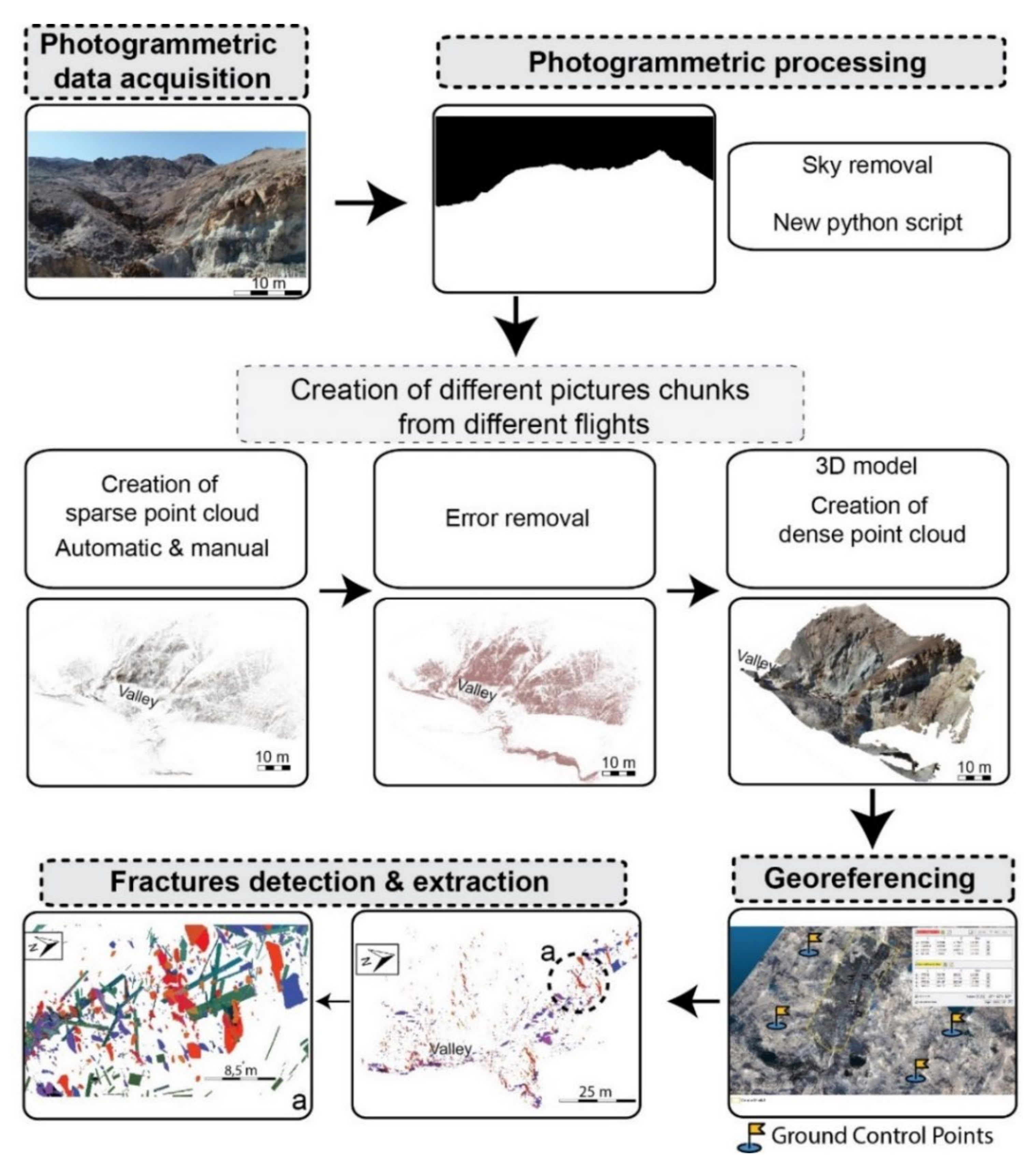
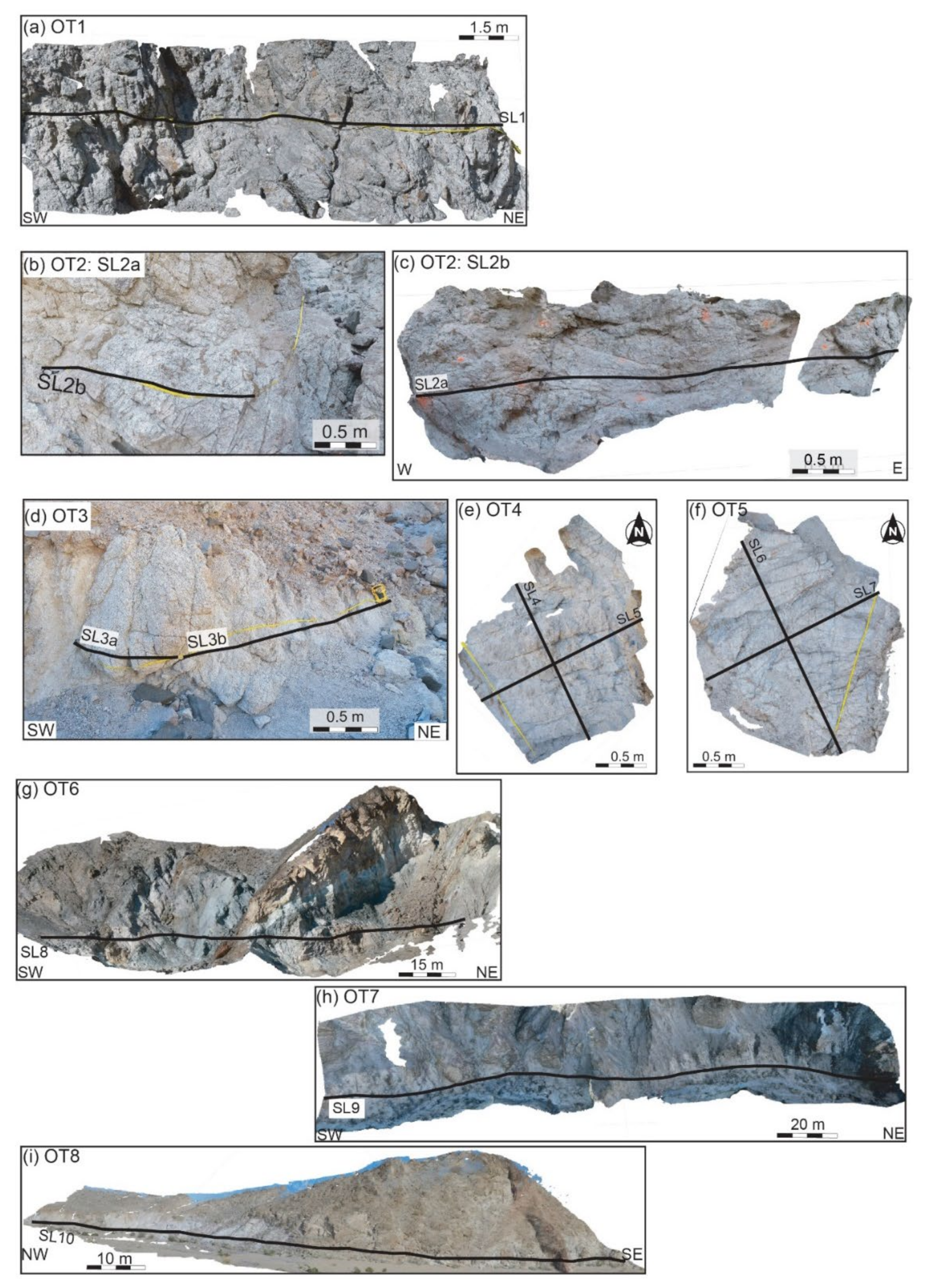
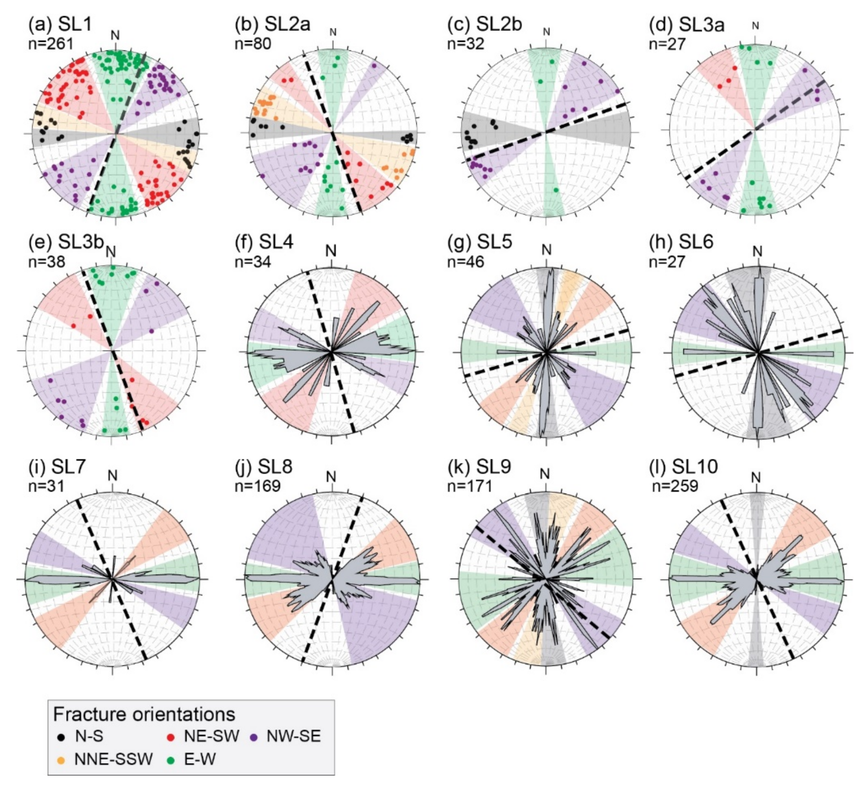
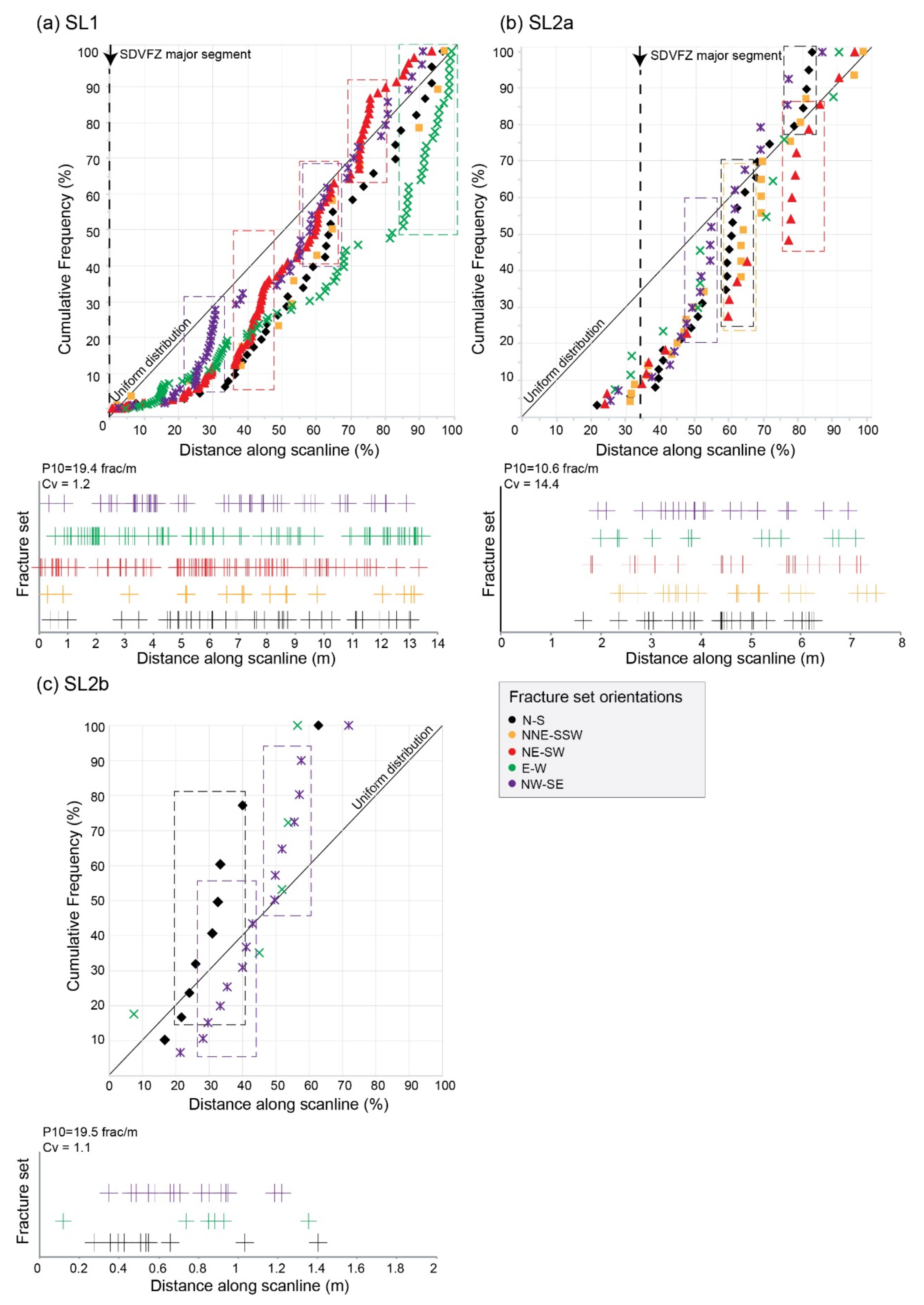
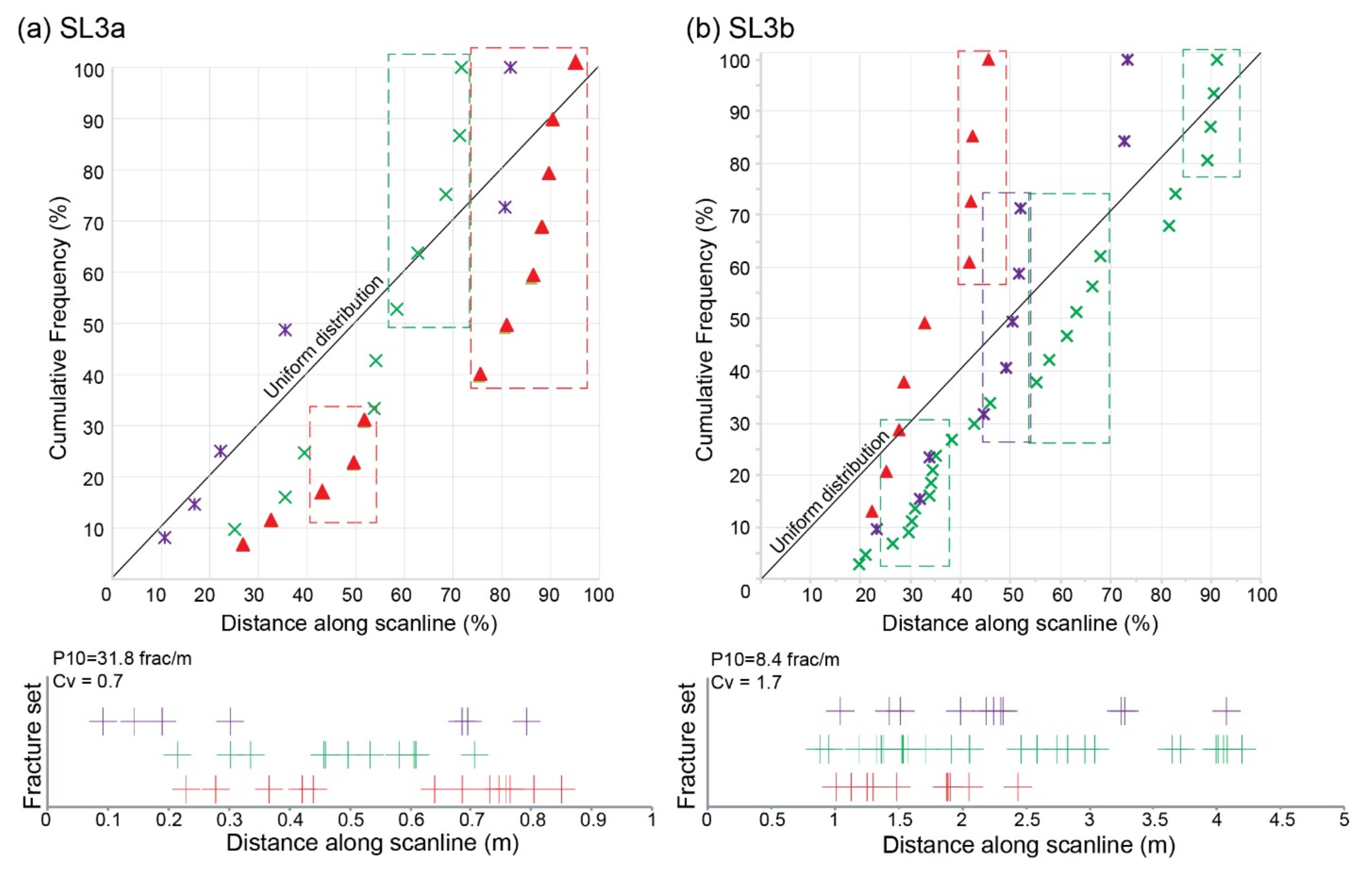
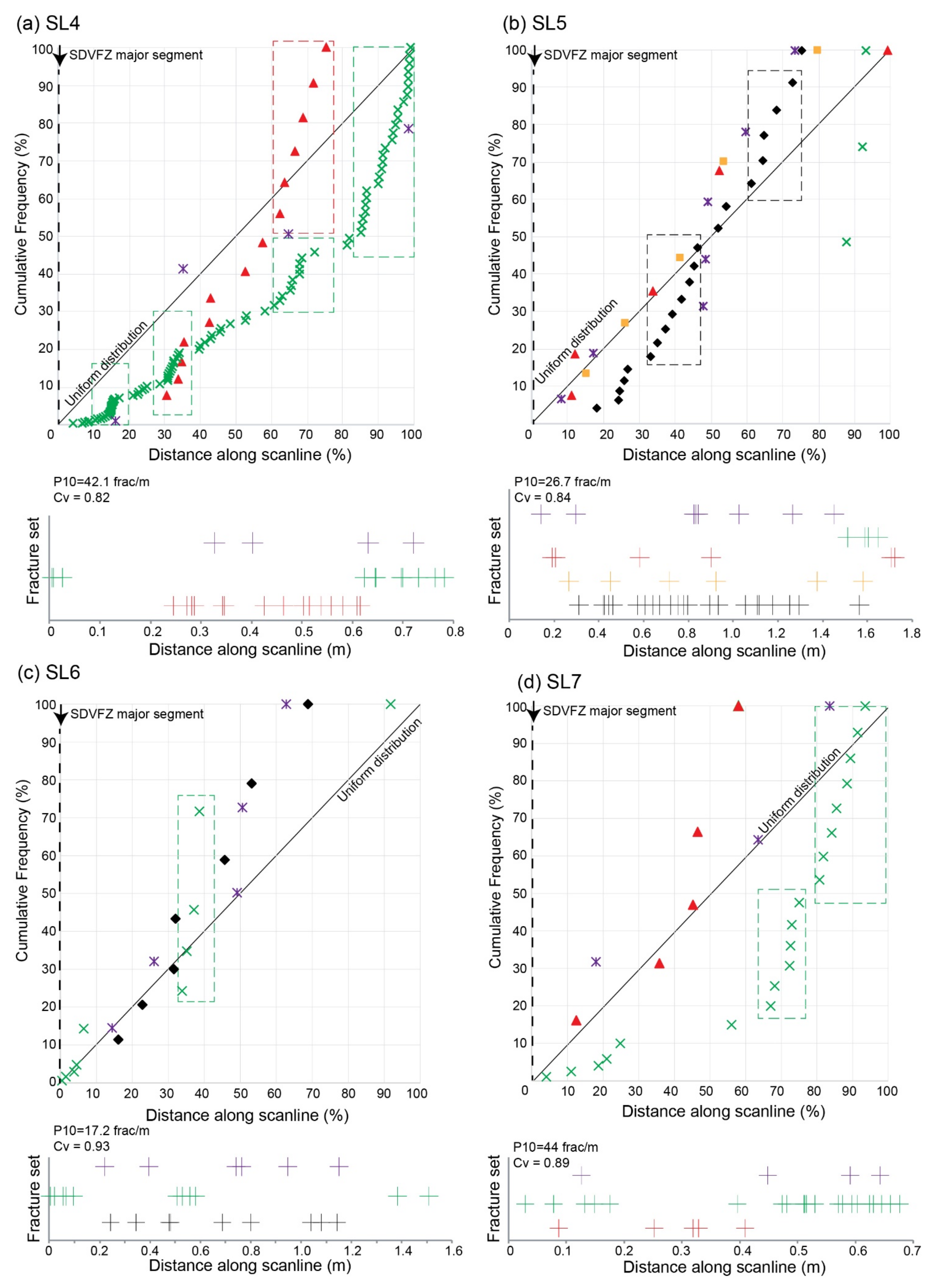

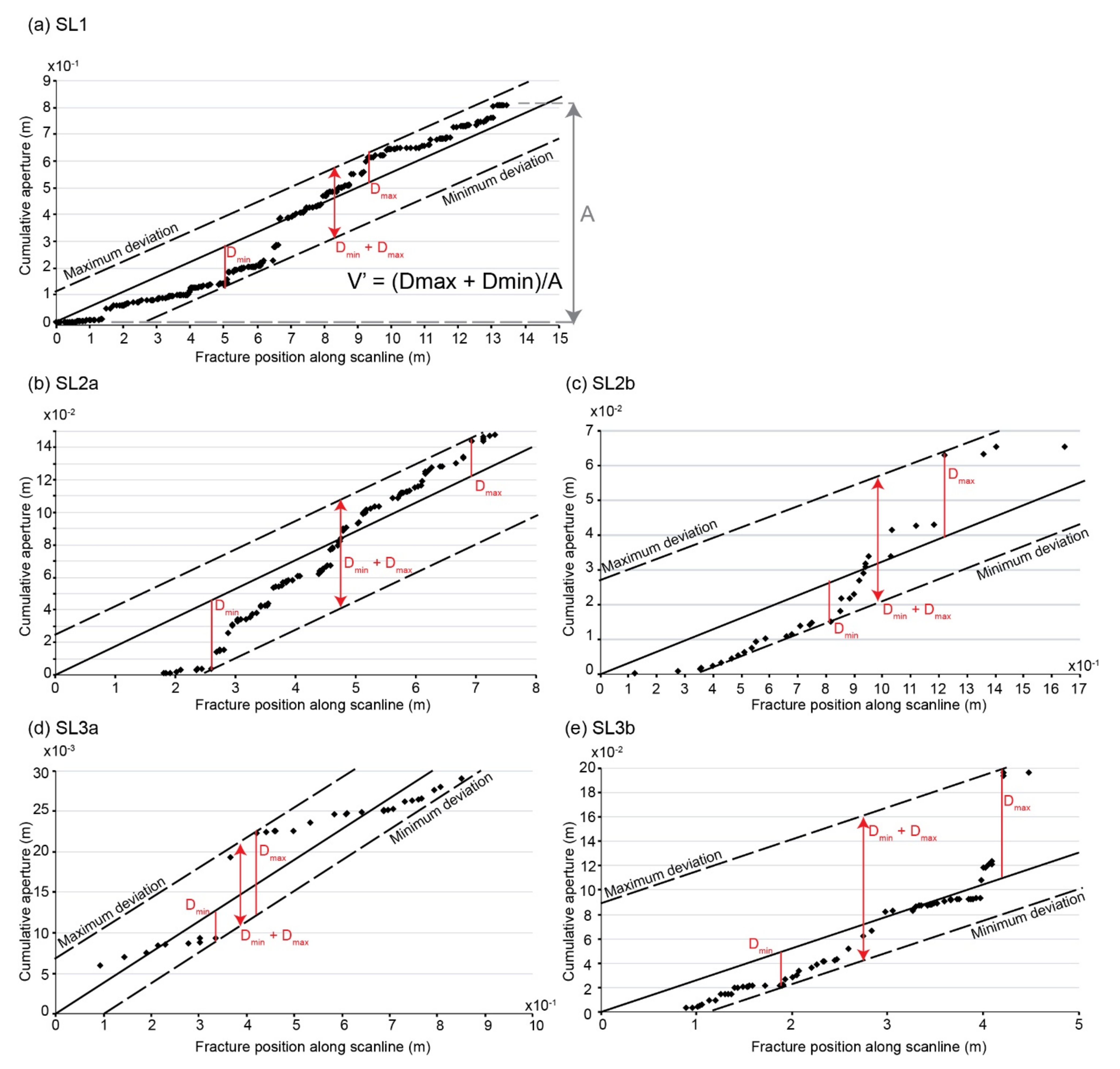


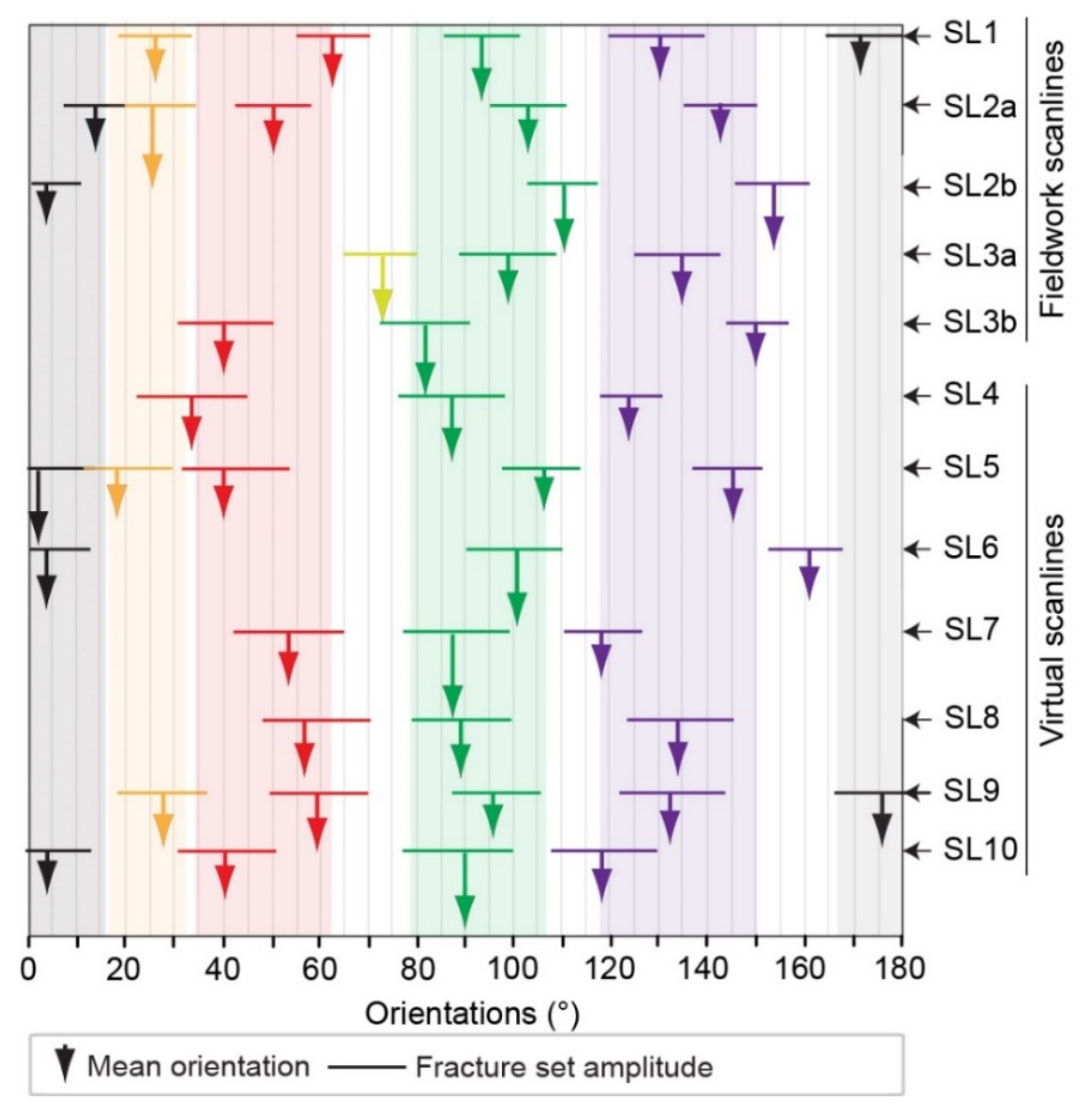
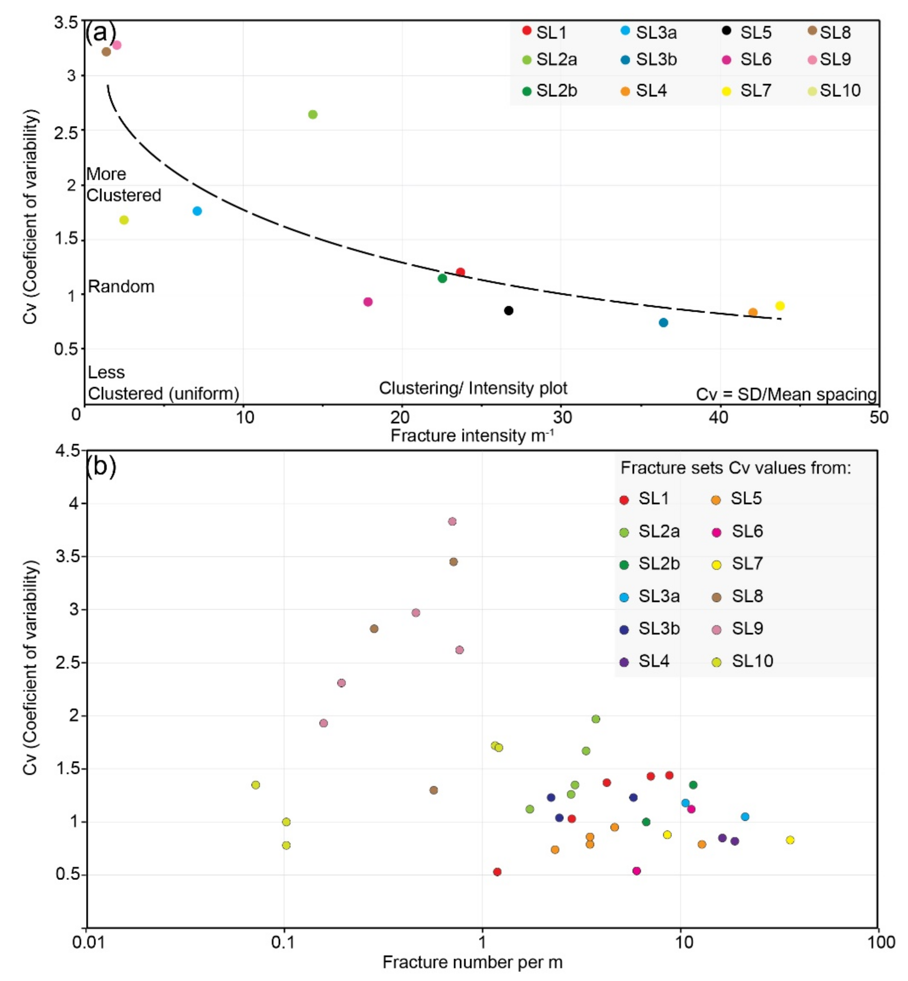
Publisher’s Note: MDPI stays neutral with regard to jurisdictional claims in published maps and institutional affiliations. |
© 2021 by the authors. Licensee MDPI, Basel, Switzerland. This article is an open access article distributed under the terms and conditions of the Creative Commons Attribution (CC BY) license (https://creativecommons.org/licenses/by/4.0/).