1. Introduction
This article describes the modeling, control system design, and test data for two prototype flight inchworm actuator (FIA) developed at the Jet Propulsion Laboratory (JPL). By flight-qualifiable it is meant that these mechanisms are designed to survive launch loads, operate in vacuum, and survive the thermal environment of space without degradation in either their performance or lifetime. One FIA is designed with a 6-micron step size and another with a 20-micron step size which features fully redundant piezoceramic (PZT) stacks and an integrated encoder. The FIA actuators are used to position various optical elements used in highly sensitive optical instruments. The FIA is a novel actuator that offers extreme dynamic range (centimeter stroke with nanometer resolution) with accuracy, power, and thermal advantages over existing motorized actuation technology such as ball screw positioners or voice coil actuators. These advantages come with the added benefit of greatly reduced complexity of the support electronics and mechanical assembly. The thermal advantages are important for optical instrument applications because of the precise alignment tolerances that must be met within the core assembly of the instrument. These advantages are due to the absence of a heat-generating electric coil and a motion gait that can end in a power-off state.
Inchworm actuators have been commercially available for some time. Physik Instrumente (PI), Burleigh, PiezoMotor, New Scale, and Cedrat [
1,
2,
3,
4,
5] offer off-the-shelf products used in ground-based optical instruments, microscopes, and lithography machines. None of these actuators, however, have been flight-qualified for space applications. The inchworm actuator described in [
6] was designed to be vacuum compatible for use in a scanning electron microscope (SEM) and was designed for long-term thermal stability, but was not required to survive launch loads as the FIA was. Moreover, this inchworm made use of shear mode PZTs which are known to suffer from severe hysteresis [
7] and have limited stroke. The FIA uses axial-mode PZTs that have much longer step sizes increasing the maximum velocity of the actuator.
The FIA consists of three sets of piezoelectric (PZT) actuators, two brake PZTs, and one extension PZT. These PZTs are used to grasp and move a runner attached to the optic to be moved. By adjusting preload rods, each brake can be configured for either a power-off or power-on parked state, which is a feature that has not been seen in previous brake designs, such as those mentioned in [
6,
8,
9,
10] which are all power-off brakes. The advantage of power-on brakes is that the holding force is generally greater than relying on the compliance of the mechanism to hold the actuator in place. The FIA brakes were designed to have 53 Newtons of holding force in the power-on state. Tightening the preload rods engages the brake without PZT extension (power-off brake), while loosening the preload rods requires PZT extension to engage the brake (power-on brake). One of the longstanding issues with inchworm technology is that actuation of the brakes causes unintended motion of the moved element. This phenomenon has been reported and characterized by other researchers such as [
6,
8,
9,
10]. The JPL FIA mechanism is no exception. The 6-micron FIA, for example, had a brake disturbance of 3 microns without significant environmental loads. This is half the step size of the actuator, and must be addressed in the design of the control, otherwise positioning performance of the actuator will be severely limited.
Although many researchers and institutions are actively developing inchworm technology [
11,
12,
13,
14,
15] most publications describe the design and performance characterization of the actuator. They are mainly concerned with metrics such as slew rate, holding force or torque, and resolution of the device. In this paper, we are less concerned with the mechanism design and performance and instead focus on the modeling and design of the control software for these devices. The mechanism design is of interest to us in so much as it has flaws, such as the brake disturbance that needs to be addressed with the control design. Some efforts have been made in this regard such as the work in [
16] where a simple electrical and elastic model of the PZT was developed. This model, however, does not consider the flexibility of the mechanism and hysteresis as in [
17,
18], and in the modeling work done in this paper. Moreover, it does not consider the different impedances of the mechanism that depend on the brake configuration. Modeling these effects, in particular the hysteresis, led to important insights as to why the brake disturbance varies significantly during slews.
Regarding control design for inchworm actuators, few if any publications cover this. The efforts in [
10] are notable but they only consider feedforward compensation of the driver PZT hysteresis. Traditional feedback control is not used and addressing the issue of brake disturbances is not mentioned. This control design in this paper considers compensation of hysteresis in terms of how it effects the scale factor of the extension PZT; in addition, estimation and compensation of the brake disturbance is addressed. These features are important since both the scale factor and brake disturbance vary during operation of the FIA inchworm. The brake disturbance was found to vary during regulation or holding of a given position, during slews or repositioning of the inchworm, and due to environmental spring loading. Compensation of the brake disturbance is a key feature of the proposed control scheme. For the 6-micron FIA device performance, the control was limited only by the resolution of the optical encoder used to measure the displacement of the actuator. For the 20-micron FIA the performance was limited by the brake disturbance, as this device had more severe variations of the brake disturbance under the test conditions used.
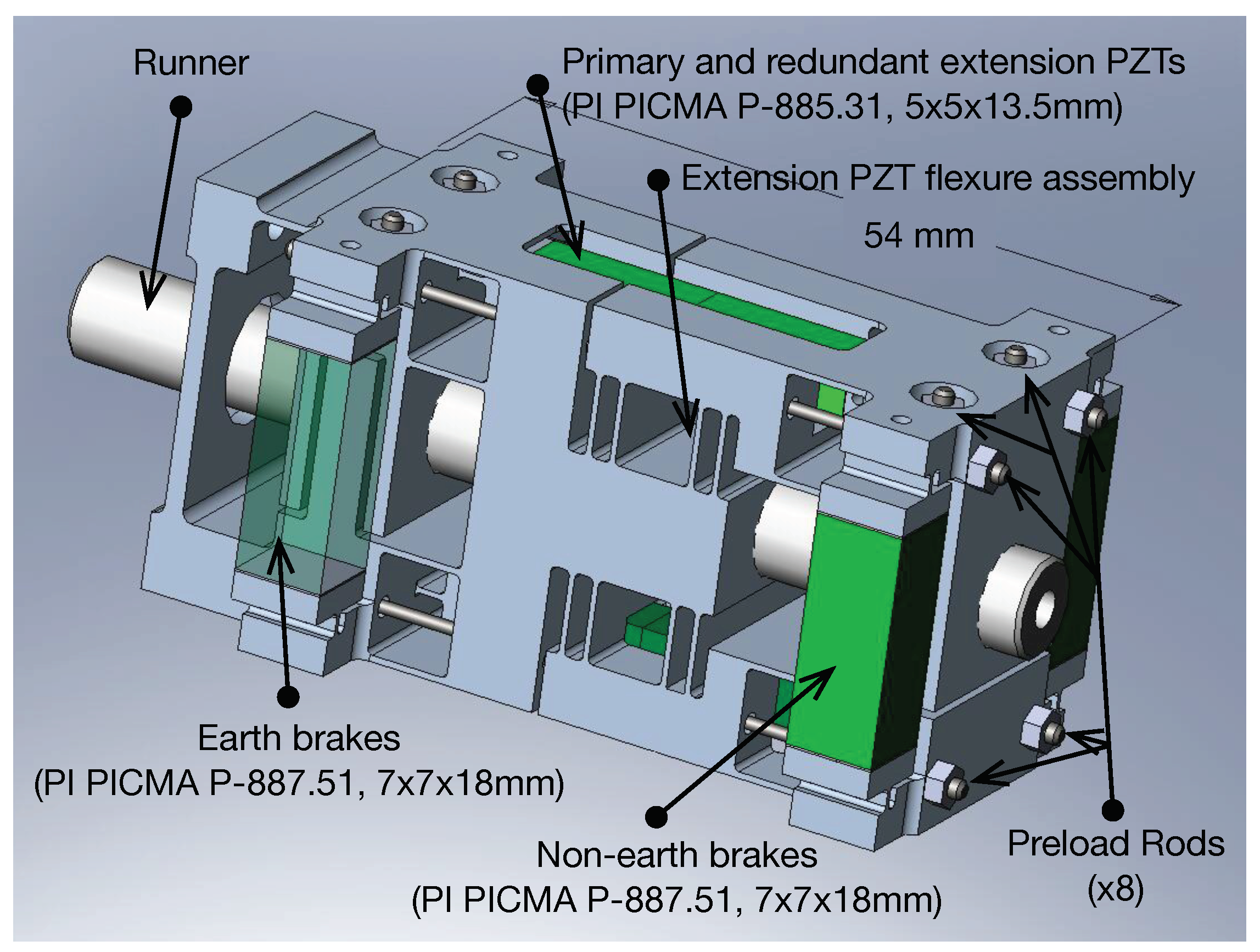
A pictorial of the 6-micron FIA actuator is shown in
Figure 1. Note the cylindrical rod running down the center of the mechanism. This rod is the moved element and is coupled to the flexure system of a mirror mount. A MicroE Mercury II optical encoder with 1.2 nanometers of quantization is used in both mechanisms to measure the position of the cylindrical runner. The brake PZT on the left is termed the earth (front) brake because it is grounded mechanically to the test jig. The second brake is connected to the earth brake through a flexure system and four preload rods. This brake is called the non-earth (back) brake and can be moved along the length of the runner by the extension PZTs. Nominally, the earth brake is set for power-off operation when engaged and the non-earth brake is set for power-on operation when engaged; this ensures a power-off state when holding position with the earth brake engaged and the non-earth brake open. The brakes operate by gripping the runner in a guillotine-like fashion. The step size of the actuator refers to the maximum amount the extension PZTs can move the non-earth brake.
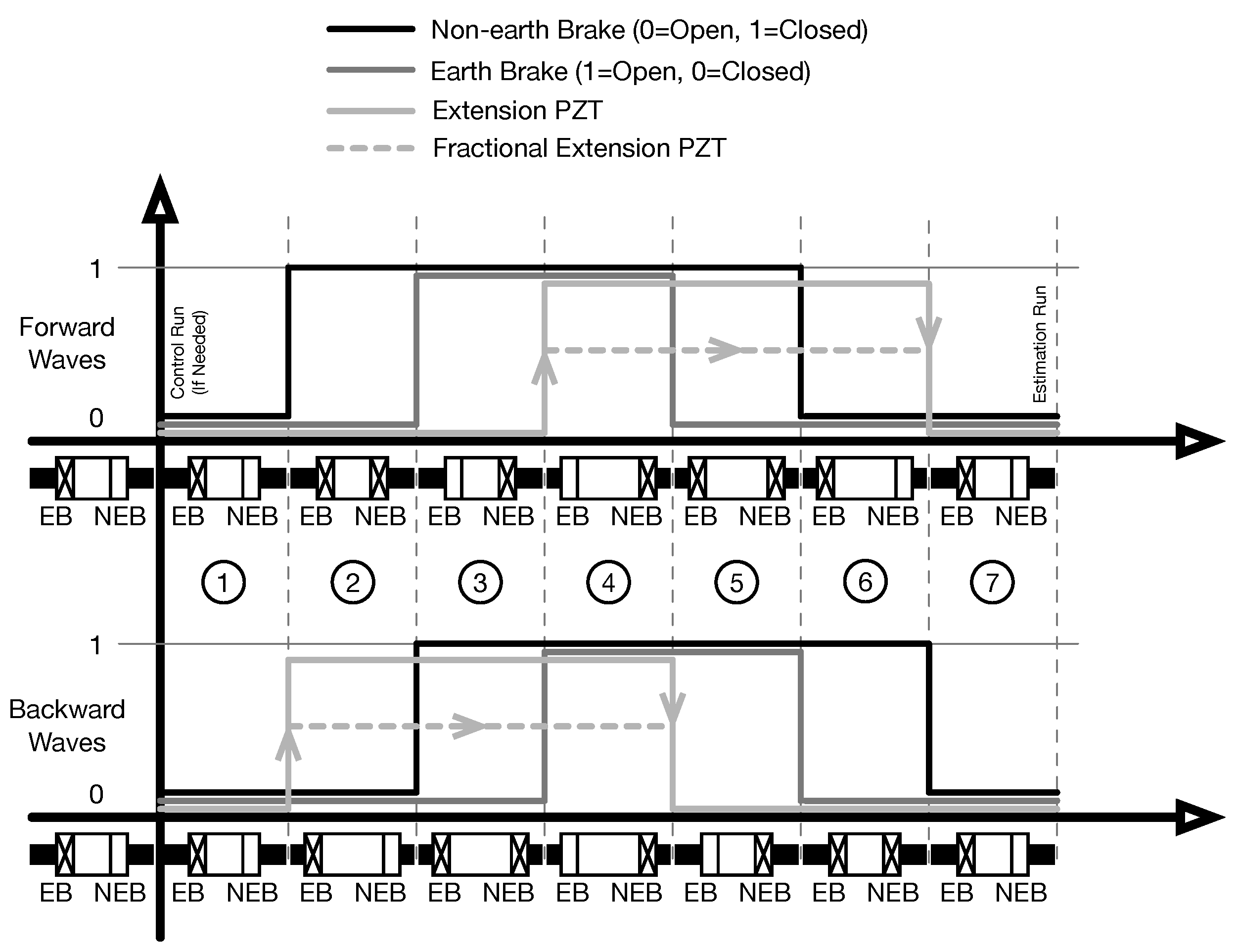
To complete one step of runner motion, the voltage waveforms to the three sets of PZTs must be coordinated correctly. The stepping gait used for testing of the FIA mechanism is shown in
Figure 2. This gait is termed the parking gait because the end state of each forward or backward step ends without power applied to the mechanism. As shown in this figure, except for phasing, the two brake waveforms are the same for both a forward step (to the right in
Figure 1) and backward step. Each brake cycle starts with the earth brake closed and the non-earth brake open. In this state the runner is held in position by the power-off earth brake. For a forward step, the first state change is the closure of the non-earth brake, followed by opening of the earth brake. This puts the mechanism in a state where the runner is held by the moveable non-earth brake. Any motion that is commanded to the extension PZTs can now take place. Once the motion occurs, the earth brake is again closed followed by opening of the non-earth brake. The non-earth brake is then repositioned to its retracted position. Backward steps are the same except prior to the start of a brake cycle the non-earth brake is prepositioned with the extension PZTs. This method of stepping allows for a step size of plus or minus the extension PZT stroke. Fractional forward and backward steps can be implemented by adjusting the amplitude of the extension waveform as shown in
Figure 2.
Encoder measurements taken before and after each step allow for determining the total amount of motion that occurred. Some of this motion will be due to the intended step size, but a significant portion of it will be due to unwanted runner motion induced by opening and closing of the brakes and positioning errors of the non-earth brake with the extension PZTs. The brake disturbances are very difficult to predict and are the primary difficulty in trying to control the position of the runner. The positioning errors are caused by uncertainty in the voltage to displacement relationship of the extension PZTs which we refer to as the scale factor of the mechanism. This uncertainty is due to the nonlinearity of this relationship which is not known prior to operation of the mechanism. Much, if not all, of this nonlinearity can be attributed to the hysteresis in the extension PZT. The control design requires knowledge of the inverse of this relationship, called the inverse scale factor. This allows the software to determine the voltage needed to move a given or desired displacement. Piecewise linear basis functions, also referred to as fuzzy basis functions, are used to accurately capture the shape of the inverse scale factor relationship. Without this accuracy, each step the mechanism takes will have an error that would have to be overcome with more iterations of the control algorithm. The control methodology described in this article estimates, in real time, both the brake disturbance as well as the inverse scale factor of the extension PZTs. Simulation and test data are presented that validate the utility of this control design.
Since moves of the FIA mechanism that involve multiple steps take longer than single step moves, this leads one to update the control input at the end of each move, instead of at end of each step, which results in an asynchronous, or variable, update rate. This is not a common situation since most control loops use a fixed update rate. As we will see in subsequent discussions, asynchronous sampling avoids saturation of the actuator and makes latencies of the plant vanish which are both important features to the performance of the mechanism.
2. Mechanism Modeling
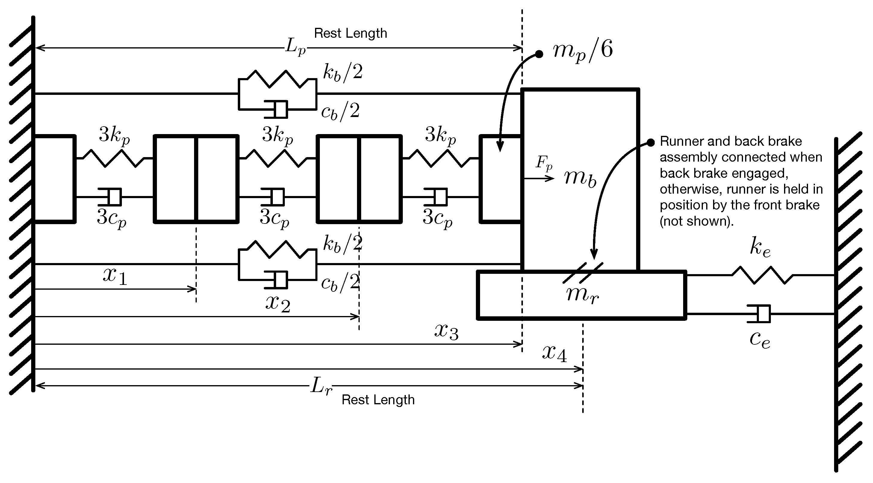
To support control code development a 1-D structural model of the inchworm mechanism was developed. The model is a hybrid differential equation depending on whether or not the non-earth brake is open or closed. When the earth brake is open and the non-earth brake is closed, the impedance of the runner mass, environmental stiffness, and damping are active along with the impedance of the PZT and flexure, otherwise when the earth brake is closed and the non-earth brake is open, only the impedance of the PZT and flexure is active with the runner held fixed by the closed earth brake. In either case, the extension PZT is chopped up into three finite elements as shown in the free body diagram of
Figure 3 [
17]. The model incorporates states to account for the PZT sub-element displacements, the non-earth brake displacement, and the runner displacement. When the earth brake is closed and the non-earth brake open, the extension PZT sees its own impedance and that of the preload rods. The runner states are physically constrained in this configuration as the earth brake is holding it in place. The equations of motion in this case can be written as,
where
,
, and
are the position states of the first, second and third extension PZT elements and
is the position state of the runner. The mass, stiffness, damping and lengths in Equation (
1) are labeled in
Figure 3. The input,
, is the force produced by the extension PZT when a voltage is applied.
is the rest length of the PZT. The last forcing term in Equation (
1) is necessary to make the equilibrium point of
equal to the rest length of the extension PZT. The states governing the runner motion,
and
, are padded with zeros to account for the fact that when the non-earth brake is open, and the earth brake closed the runner is constrained from moving.
When the non-earth brake is closed and the earth brake is open the runner states are no longer constrained and we have,
where
is the resting position of the runner and
, where
is the runner mass.
and
are the stiffness and damping of the environment as shown in
Figure 3. In the development of Equations (
1) and (
2) discussion of the PZT preload rods is not necessary since this preload merely effects the resting length of the PZT. Please note that by dividing the PZT into sub-elements we capture the high frequency behavior of the surge modes. For this application, however, the surge modes are not important.
Two other brake states must be considered. When both brakes are closed, a ground loop is created and no change in any of the state variables is possible. In this case, the left-hand side of Equations (
1) and (
2) is set to zero. The fourth brake state is when both brakes are open. In this case, the runner would slip and come to its equilibrium position as determined by the rest length of the environmental spring. This case need not be considered because it is not part of nominal operation of the mechanism. Referring to the stepping gait in
Figure 2 we can confirm that the only brake states used are (1) when the earth brake is closed and the non-earth brake open (2) when both are closed and (3) when the non-earth brake is closed and the earth brake open. Determination of which set of equations, (
1) or (
2), to integrate is based on the voltage levels applied to the two brake PZTs. A threshold of 50.0 Volts (100 Volts is full scale for the PZTs used) was used to change the state of the brake from open to closed and vice versa. The mechanism model is initialized in its equilibrium state of,
The extension PZT force input,
, to Equations (
1) and (
2) is controlled by the extension PZT voltage waveform. PZT ceramics suffer from a significant amount of hysteresis which effects the scale factor of the FIA mechanism. To capture this effect, we used the approach discussed in [
17] with a hysteresis model developed in various publications including [
7,
19,
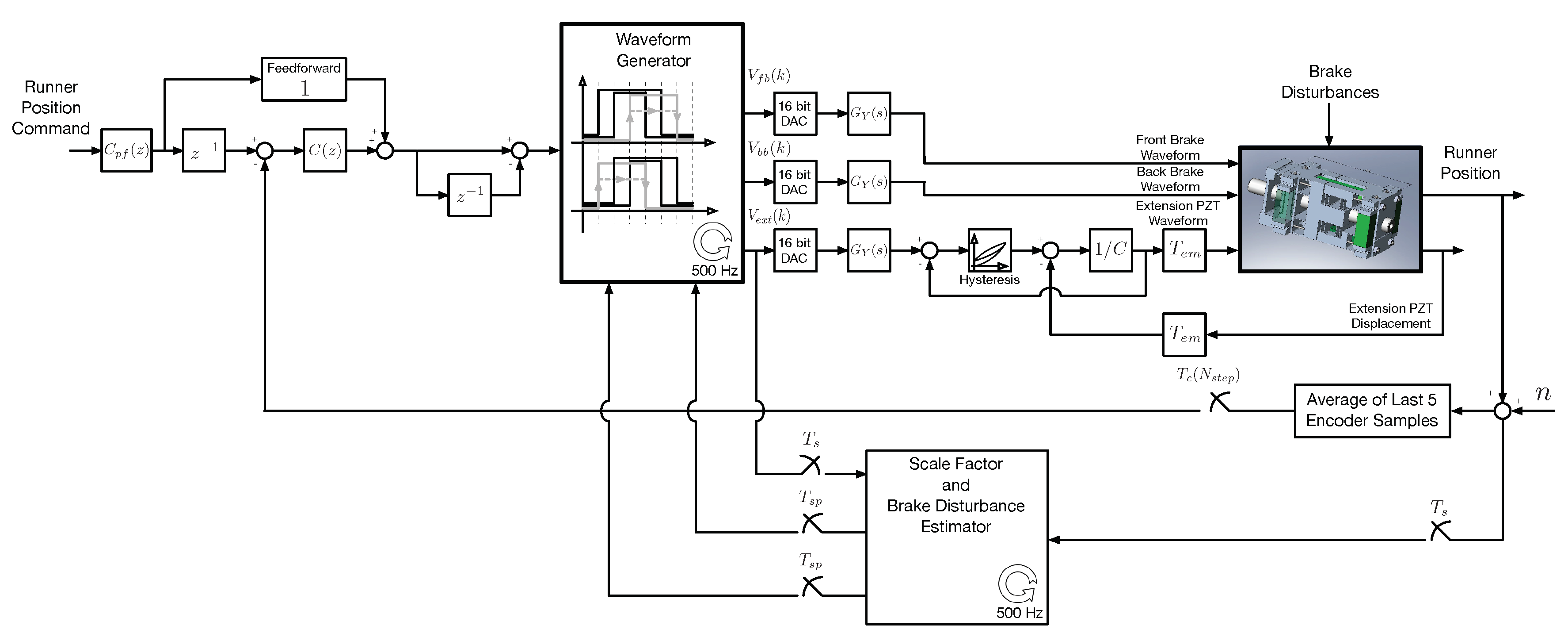
20]. The structure of this model is shown in the control block diagram in
Figure 4. The PZT is a two-port transducer with voltage and charge as the effort and flow variables in the electrical domain and force and displacement as the effort and flow variables in the mechanical domain. The effort and flow variables in each domain are related by the piezoelectric constant
with units of Newtons/Volt or Coulombs/meter. The displacement to charge feedback depicted in
Figure 4 is explained by the fact that if an external force is applied to the PZT a voltage is produced that opposes this force. The voltage is generated as a consequence of the charge feedback and capacitance of the PZT,
C, since
.
Figure 4 also illustrates that PZT hysteresis is an electrical domain phenomenon that maps voltage to charge [
17]. Backlash basis functions are fit to this input output data using techniques developed in [
7,
19,
20]. The voltage and charge data for this fitting process is generated from low frequency amplifier voltage and PZT displacement data (Data taken without the flexure or environmental impedance active.) which is mapped to the input and output of the hysteresis using knowledge of the various physical constants, the capacitance,
C, piezoelectric constant,
, and stiffness of the PZT,
.
The two brake and extension PZT voltage waveforms generated by the control software are converted to the analog domain using 16-bit DACs with a 0–10 Volt signal as shown in
Figure 4. The transfer function,
, includes smoothing unity gain Bessel filters with a corner frequency of 300 Hz and the PZT amplifier gain of 10 with a roll-off at 475 Hz. The Bessel filters and amplifier serve to reduce the high frequency energy applied to the mechanism decreasing fatigue on the flexures and PZT ceramic.
Alternative Model
Extensive testing with the mechanism revealed an alternative discrete time model of the inchworm actuator. From a mathematical point of view the actuator is nothing more than a mechanical adder of displacements. The new displacement,
, is just the old displacement plus the current step size,
where
z is the complex Z-transform variable. We have broken the step size into two parts, the first being the commanded step size caused by the control input,
, and the second,
, the step size motion caused by the brake disturbance. The input,
, is the fraction of a full forward step, 1, or a full backward step, −1. The function,
, was found to be nonlinear due to hysteresis in the extension PZT and due to other mechanical effects.
The model in Equation (
4) has some advantages over the model described in the previous section. It directly includes the effect of brake disturbances and is much faster to integrate since it is free of high frequency structural modes. It has the disadvantage of not modeling the behavior within a given step. This prevents its use in estimator development, but it is of use in the plant modeling for compensator design.
3. Control System Design
The block diagram in
Figure 4 illustrates the three different components of the FIA control system, the waveform generator, the compensator, and an estimator. The waveform generator sends voltage signals to the brake and extension PZTs based on commands from the feedback and feedforward compensator and updates provided by the estimator. The waveform generator will send waveforms that implement either a forward or backward step based on this command. The waveform generator pushes the brake and extension waveforms out the three DACs as square waves at a rate of 500 Hz. Each step takes
seconds giving 100 samples per step for each waveform.
The runner position is measured at a sample rate of
seconds, the same rate at which the voltage waveforms are generated. The measurement noise,
n, depicted in
Figure 4 is the result of encoder quantization. The quantization interval of the encoder was 1.2 nm giving a uniform distribution of the noise with a standard deviation of
.
The estimator is used to update knowledge of the mechanism inverse scale factor and brake disturbance during operation. The estimator takes samples of the extension voltage and encoder at 500 Hz. These samples are processed, and estimates are updated at the end of each step, every seconds.
3.1. Discrete Event System
For control, measurements of the encoder position are taken at the end of the stepping gait when the mechanism is in its parked state. Each measurement of the encoder position is the average of the last five encoder samples from the previous step. This averaging gives a bit more resolution of the feedback signal. Since each move command issued by the control can be several steps in length or a single step if only a fractional correction is necessary, the sampling interval,
, in
Figure 4 will be variable. This was done for two reasons. First, sampling at variable or asynchronous times depending on how many steps are taken is transparent to the discrete control system. This does not affect loop stability since the stability of a discrete time system (compensator and plant) does not depend on the specific times at which the compensator difference equations are iterated. Second, sampling and calculating a new control input at a regular interval, say at the end of each step, will introduce a saturation nonlinearity at the output of the compensator if a multiple step move is requested. This happens because the mechanism cannot complete more than one step before the next move command is calculated. If a multiple step move was commanded prior to the current control cycle, one would have to overwrite the last command before it is finished with the new one effectively limiting the commands to a single step. This introduces a saturation nonlinearity in the loop structure. Alternatively, one could wait for the previous multiple step command to be fully executed then calculate a new move based on the encoder measurement at the end of the move. This removes the saturation from the control loop.
3.2. Feedback and Feedforward
The controller calculates an incremental distance to move based on the encoder feedback and reference position. The distance to move is the difference between the accumulated position target and its previous value as shown at the input to the waveform generator in
Figure 4.
Since simply cycling of the brakes during the stepping gait causes a surprisingly large amount of unwanted runner motion, without any control the runner would drift off in a ramp-like fashion due to these disturbances. To counteract this ramp disturbance, the compensator,
, in
Figure 4 was configured with two integrators. To stabilize the phase lag that results from these two integrators a zero was added just before the open loop crossover. This crossover was roughly 0.3 Hz resulting in a closed loop bandwidth of approximately 0.5 Hz when single steps are taken. A prefilter was included,
, to smooth the reference positions and cancel the closed loop resonance of the feedback loop. In addition, a feedforward path was added to speed convergence of the control system to the reference position. The extra delay placed in the command path is used to prevent the feedback loop from seeing the large error caused by a new command until after (one iteration later) the feedforward command has been executed and the error becomes smaller. This reduces overshoot of the transient response and reduces the convergence time of the control system. Two flags are set in the control software to select or deselect the feedforward channel and prefilter.
Alternatively, one could use a single integrator and rely on the brake disturbance estimate for compensation of the brake-induced motion. This would greatly improve the gain and phase margins of the feedback loop but is susceptible to errors in the disturbance estimate. Without prior experience on how successful the brake estimation would be the path taken was to use the two integrators and later assess the viability of using a single integrator.
3.3. Estimation
The estimation task runs at 500 Hz and provides state updates at 5 Hz, or one update per step of the mechanism. For a multiple step move, the estimates will be ignored for all but the last step. During the first 99 time samples of a step the estimation task does nothing but collect samples of the encoder and extension PZT voltage waveform. The extension PZT waveform is sampled from inside the software, before it is converted to volts. The encoder and extension PZT samples are placed in 100 element ring buffers with the most recent samples being placed in the last element of the array. On the 100th sample of a step the last encoder and extension waveform samples are placed in the arrays, raw measurements using these samples are formed, and the Kalman filter is iterated. The updated state estimates produced by the filter are then made available to the control task which executes after the first sample of the next step.
The raw measurements formed by the estimator are assembled by first taking the average value of the encoder and extension waveforms during each of the seven distinct segments of brake activity shown in
Figure 2. If we denote the samples of the encoder and extension wave as,
and
, where
, the segment average values are given by,
for the encoder wave and,
for the extension wave. These segment averages are then used to form the raw measurements used by the Kalman filter. In the case of a forward step the raw measurements are given by,
For a backward step, to account for the different time slot of the runner displacement, the raw measurements are given by,
The first measurement in these equations gives the commanded displacement of the runner in terms of a normalized percentage of full step motion with 1 used to represent a full forward step and −1 a full backward step. The second measurement gives the actual runner motion achieved by this command due to the extension PZT movement. The third measurement gives the unintended motion of the runner during the step due to the brake disturbances. Please note that to form this measurement the actual motion caused by the control command is subtracted from the total motion during a complete cycle of the stepping gait. The estimator is used to create a map between the actual motion of the runner,
, (X-axis) and the commanded motion of the runner,
(Y-axis). This relationship is the inverse scale factor of the mechanism and is used in the controller to determine the extension command for full step sizes and fractional step sizes. To model this mapping the estimator uses piecewise linear segments constructed from properly weighted triangular basis functions. The estimator solves for the weights of these functions. These triangular basis functions are also called fuzzy membership functions. The exact set of functions is given below where
u is used to denote the input variable, in this case,
. The points
are a priori specified parameters that represent the center location of each triangular membership function. These centers were chosen to be symmetric about the
point.
Note the zero point was excluded from support to constrain the solution to pass through zero. The support at either extreme end of the input is linear resulting in data near the ends of the mapping determining the slope and bias at all extremum points. The estimator is also used to smooth measurements of the brake disturbance (
9) and (
12) which are directly measured. With these preliminary comments the measurement equation used in the estimator is,
where,
The first ten elements of
are the scale factor weights and the last element of
is the brake disturbance estimate,
. The process model used was simply,
which allows for tracking of time varying states. Since the scale factor was more stable than the brake disturbance, the covariance of
associated with the scale factor parameters was chosen to be small relative to the value used for the brake disturbance state. The filter update equations for the state and covariance are given by [
21],
where the Kalman gain
is given by,
The propagation of the state and covariance estimates between measurements was done using,
Two flags are available in the control software to select or deselect usage of the scale factor and brake disturbance estimates in the control.
3.4. Waveform Generation
Waveform generation is the process of taking the incremental move command generated by the controller and concatenating the proper waveform segments for each move. Each move will generally consist of several full steps, either forward or backward, and a single fractional step in the same direction. Once the runner position is close to its reference position the moves will settle to single fractional steps so long as the disturbance is less than the full step size.
The first step in waveform generation is to determine the number of steps to take. Before this can be done estimates of the forward and backward full step distances must be made. This was done by using a simple bisection algorithm on the estimated inverse scale factor function which can be expressed by,
where
is the most recent vector of scale factor parameters output from the estimator, i.e.,
. The left-hand side of this equation is the
or the fraction of a commanded full step. To find the forward step size the roots of
were found numerically. To find the backward step size the roots of
were solved for. To account for the effect of the brake disturbance on the respective step sizes Equation (
21) is evaluated using
in the regressor,
. This shifts the scale factor function to the right or left, increasing or decreasing the forward step size, respectively. A similar statement can be made for the backward step size. The number of steps to take is then calculated using,
where
is the commanded distance to move and
and
are the estimated forward and backward full step distances solved using the bisection procedure. The
operator rounds to the nearest integer towards zero. This rounding operation makes
the number of full steps to take. The remainder fractional distance to move,
, is calculated using,
The fractional step size to move a distance of
is then calculated using,
Once and are determined the full waveform, including brake and extension PZT voltages, can be concatenated from full step waves and one fractional step wave with the amplitude of extension wave modified by .
4. Simulations
For simulation purposes the brake disturbance was added to
as an extra force in Equation (
2). Although all brake transitions will cause some movement of the runner, for the simulations it is sufficient to add the brake disturbance only when the non-earth brake is closed, and the earth brake is released. For a forward step this happens between segments 3 and 2 shown in
Figure 2 and between segments 4 and 3 for a backward step. The extra force added was 175 N which resulted in a runner displacement of about 5.0 microns. 5.0 microns was chosen because it is a relatively small fraction (25%) of the total stroke and because it was representative of the actual brake disturbance level for the 20-micron FIA. The control function uses the disturbance and scale factor estimates updated using waveform data during the previous step and uses the last averaged encoder measurement,
, from the previous step as the feedback signal.
To highlight the challenges associated with controlling this mechanism and the features of the control system that address these challenges a comparative simulation is presented that illustrates the utility of the feedforward and estimation.
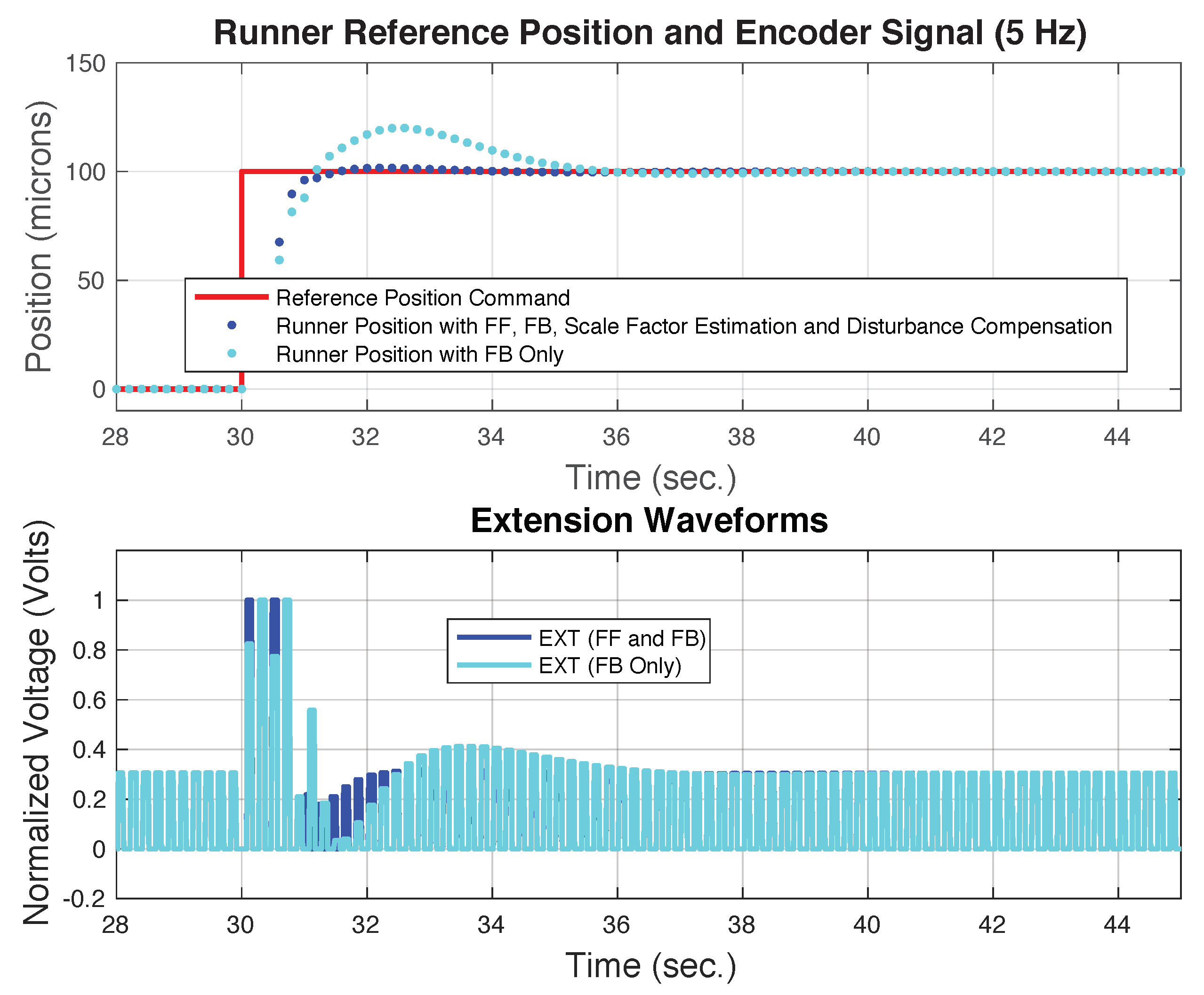
Figure 5 shows the results of this comparison. In this figure, the step response of the control system with feedforward, feedback, scale factor estimation, and disturbance compensation is compared to the case of using feedback only. In both cases the prefilter shown in
Figure 4 was removed as well as the delay in the case of the feedback only option. Removing the prefilter allows the feedforward to have a more significant effect and including it with the feedback only case has a surprisingly minor effect on the transient response since most of the transient error is caused by the disturbance response not the reference input response. This happens because the brake disturbance changes as the inchworm starts to move. This phenomenon will be demonstrated in both simulation and in test data that will be presented later. In
Figure 5 we see that the transient response takes less than 3 s to converge and stay within 1 micron of the target for the case that uses feedforward and over 7 s for the case with feedback only. This is over a factor of 2 improvement in the settling time when feedforward is used. This happens because the initial feedforward move gets the actuator close to the target before the feedback response starts. This is a significant advantage since the initial error that the feedback control sees is much smaller after the feedforward move has occurred. The smaller this initial error the more benefit the feedforward action will have. This speaks to the benefit of using the scale factor estimation and disturbance compensation since both features will result in a more accurate initial move when using the feedforward.
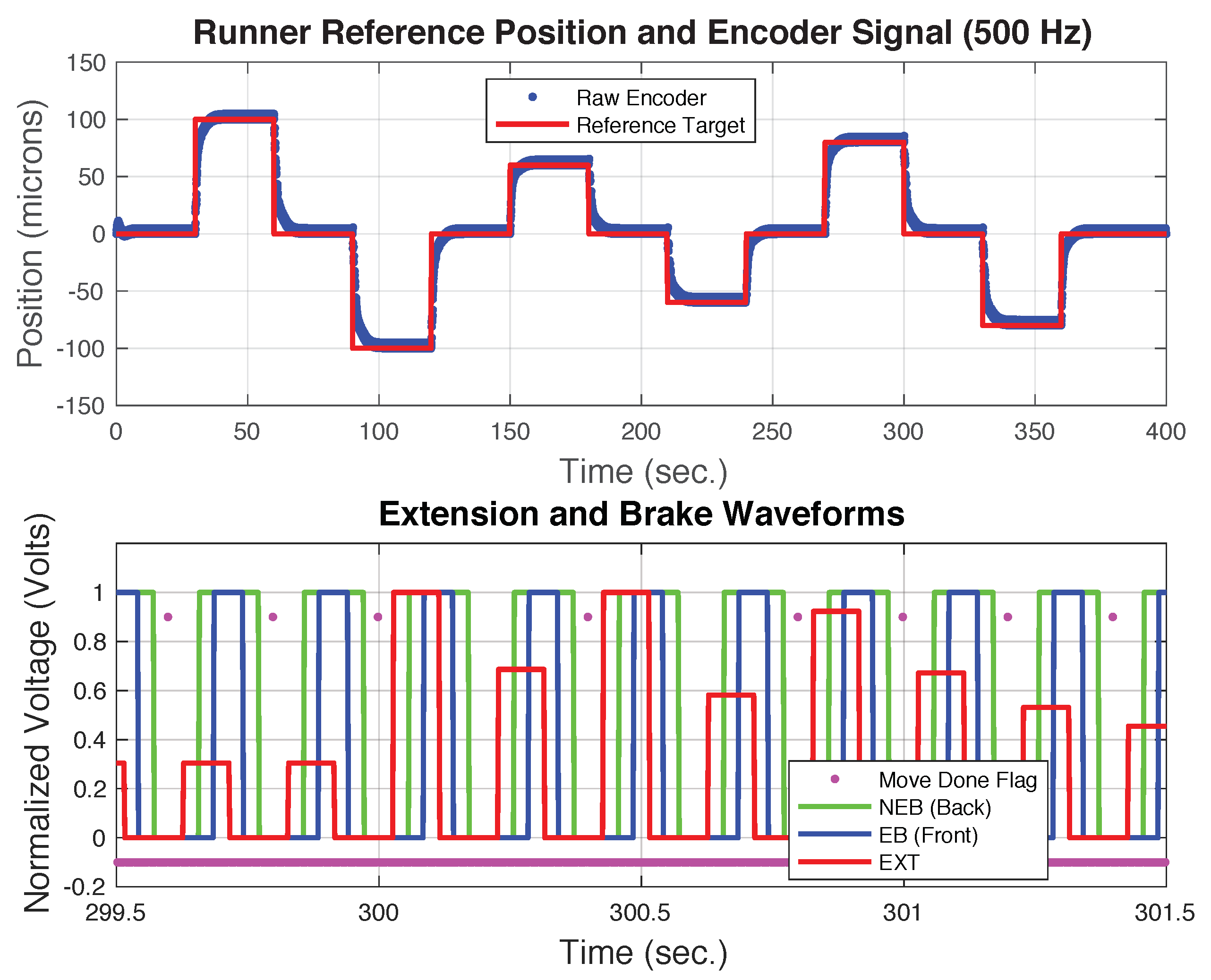
Next we look at the simulated performance of the 20-micron FIA using the feedforward and prefilter as depicted in
Figure 4.
Figure 6 shows the simulated position command and encoder signal as well as the brake and extension waveforms near
s. The encoder signal has a 5-micron thickness due to the brake disturbance within a step. When a large change in the position command is issued the controller can decide to make multiple step moves. This is shown in the bottom subplot in the first two moves after 300 s. Each of these moves consists of one full step followed by a fractional step. As the error signal gets smaller the control system settles to single step moves. Note the use of the prefilter smoothes the position command a greatly reduces the number of multiple step moves needed. Before the move at 300 s the control system has settled into a backward move of 5.0 microns or fractional step of about 0.3 to cancel the forward movement caused by the brake disturbance.
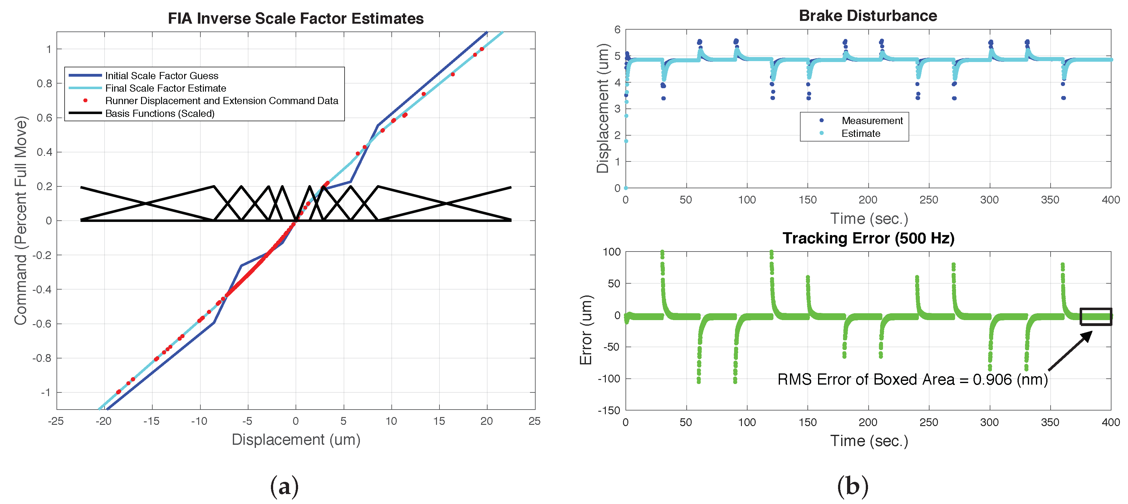
Figure 7a,b show the estimation results and residual servo error for this simulated case. In
Figure 7a both the initial and final inverse scale factors are shown along with the
and
data used to update the inverse scale factor. The final scale factor has a slight nonlinearity caused by hysteresis in the extension PZTs. The basis functions used to estimate the scale factor are also shown in this figure with denser support near zero because the function is expected to be more nonlinear in this region.
The top subplot of
Figure 7b shown the brake disturbance measurement and estimate. The brake disturbance is a constant 5.0 microns in the forward direction except during the large slews. During the slews, the brake force is acting with the extension PZT in different states. Apparently, the force to displacement response of the extension PZT is highly nonlinear and depends on the length of the PZT when the force is applied. Just before the slew, the mechanism is taking backward steps of 5.0 microns with the brake disturbance acting when the PZT is extended by 5.0 microns. Just after the slew, the first step, for example, is a full forward step with the brake disturbance acting with the PZT fully retracted (0.0 microns of extension). The extension state when the earth brake is released has a significant effect on the displacement caused by the disturbance force. Interestingly, the same disturbance behavior is seen in the test data and adds to the difficulty of controlling this device accurately during tracking maneuvers.
The bottom portion of
Figure 7b shows the tracking error,
, during the command trajectory. Ignoring the transient errors, at steady state the RMS error is less than a nanometer which suggests the simulated performance is limited only by the encoder resolution of 1.2 nm. One point of interest here is that during nominal operations the stepping of the FIA would be halted as soon as the servo error goes below some desired threshold keeping the error signal constant and reducing jitter of the optic caused by the interstep brake disturbance.
5. Test Data and Control Performance
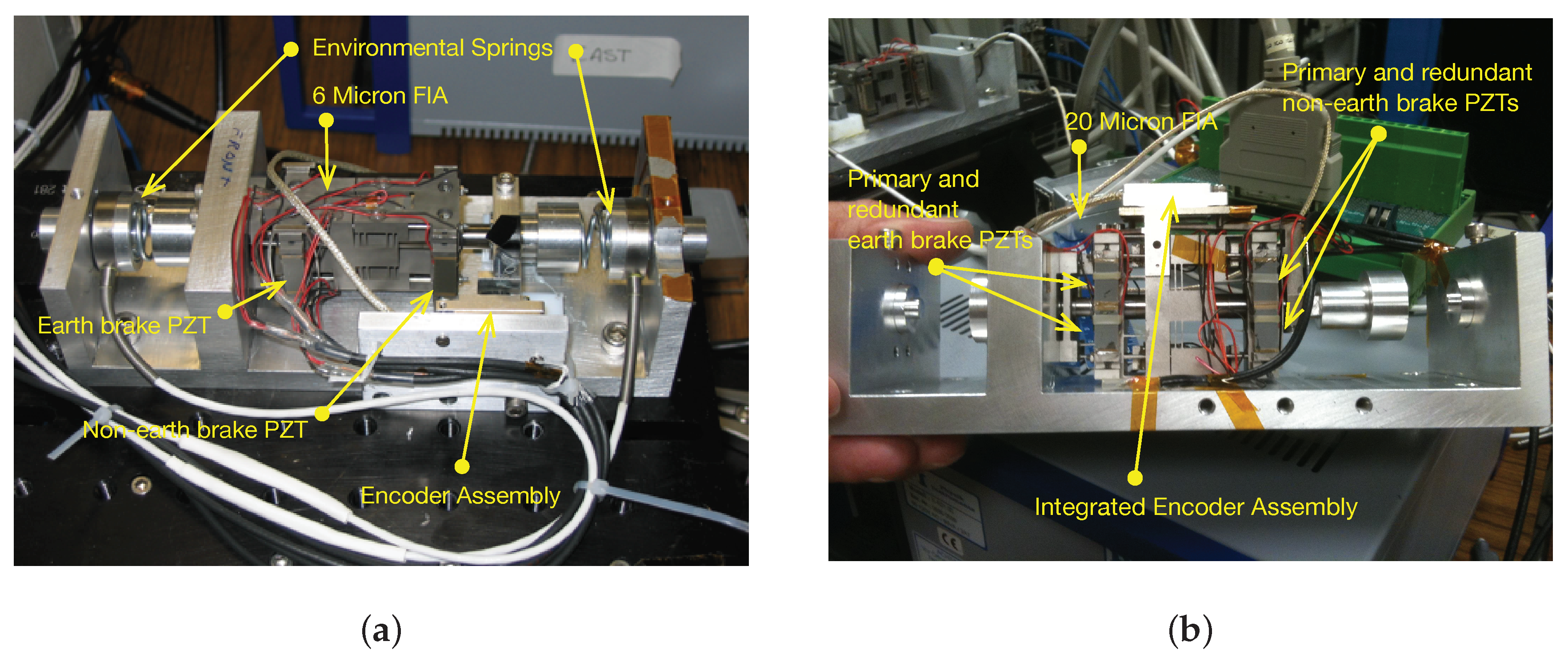
Photographs of the 6- and 20-micron FIA mechanisms are shown in
Figure 8. Two springs on either end of the test jig are used to simulate the impedance of the mirror mount’s flexure system. These springs can be seen in the photograph of the 6-micron mechanism (They are removed in the photo of the 20-micron FIA mechanism.).
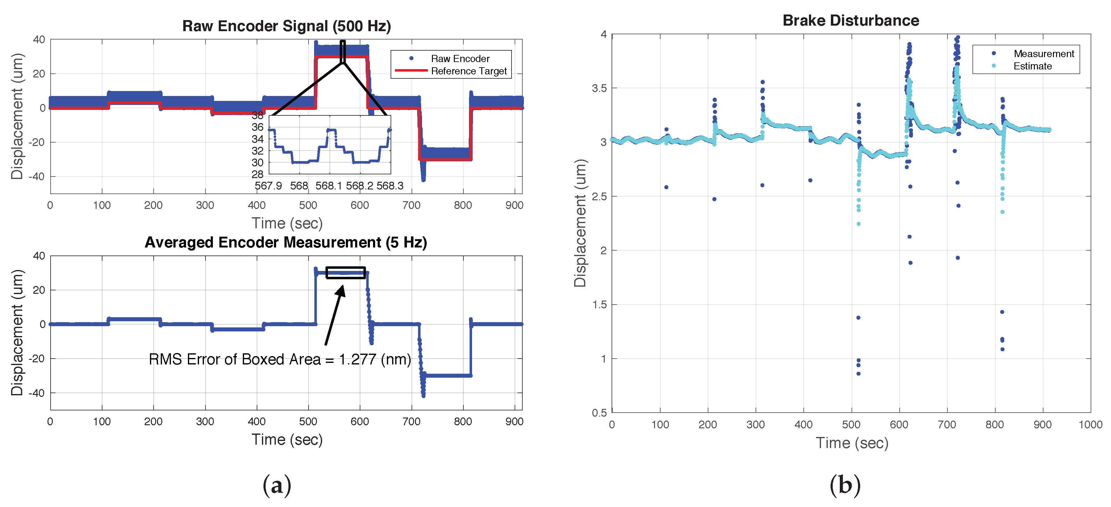
Figure 9a,b illustrate the performance of the 6-micron FIA mechanism using the double integrator with asynchronous sampling. The feedforward was used without prefiltering of the reference position commands. Offline estimates of the mechanism scale factor with fixed forward and backward step size estimates were used. The estimator and disturbance canceling scheme outlined in the previous sections were not used for these tests. The burden of canceling the brake disturbance was achieved using only the double integrator control.
The top subplot in
Figure 9a shows the step response of the mechanism for 3.0-micron moves that are less than the step size of the mechanism and 30.0-micron moves that are greater than one step of the mechanism. The ∼7.0-micron thickness of this plot is the result of the brake cycling moving the runner within a single step of the mechanism. The inset plot shows a closeup of two full steps of the mechanism demonstrating that each change of the brake state has an associated movement of the runner. The transition just after 568.1 s is the intended motion of the backward step. The other transitions are caused by brake disturbances. The averaged encoder measurement,
, which is used for control and made at the end of each move is shown in the bottom subplot of
Figure 9a. This measurement shows less variation since it is always made during the same (last) segment of the stepping gait. In fact, the RMS error of this data in the boxed region was similar to the encoder quantization of 1.2 nm. The overshoot for the forward moves in this figure is less than that for the backward moves. This is because the feedforward component of the controller used a forward step size estimate that was more accurate than the backward step size estimate.
Figure 9b shows the brake disturbance during this experiment which has an average per step disturbance of ∼3.0 microns, about half of the 6-micron step size. During regulation, the disturbance shows some slow variation but is relatively constant. During slews, the disturbance changes quite a bit, which is consistent with the simulation results. Given the size and slew variability of the brake disturbance performance would be greatly enhanced with active disturbance estimation and cancelation as proposed in this paper.
The 20-micron FIA mechanism was designed to have a larger step size, redundant PZTs, and integral encoder mounting. In addition, a hardened carbide runner was used with this mechanism whereas the 6-micron device used a stainless steel runner.
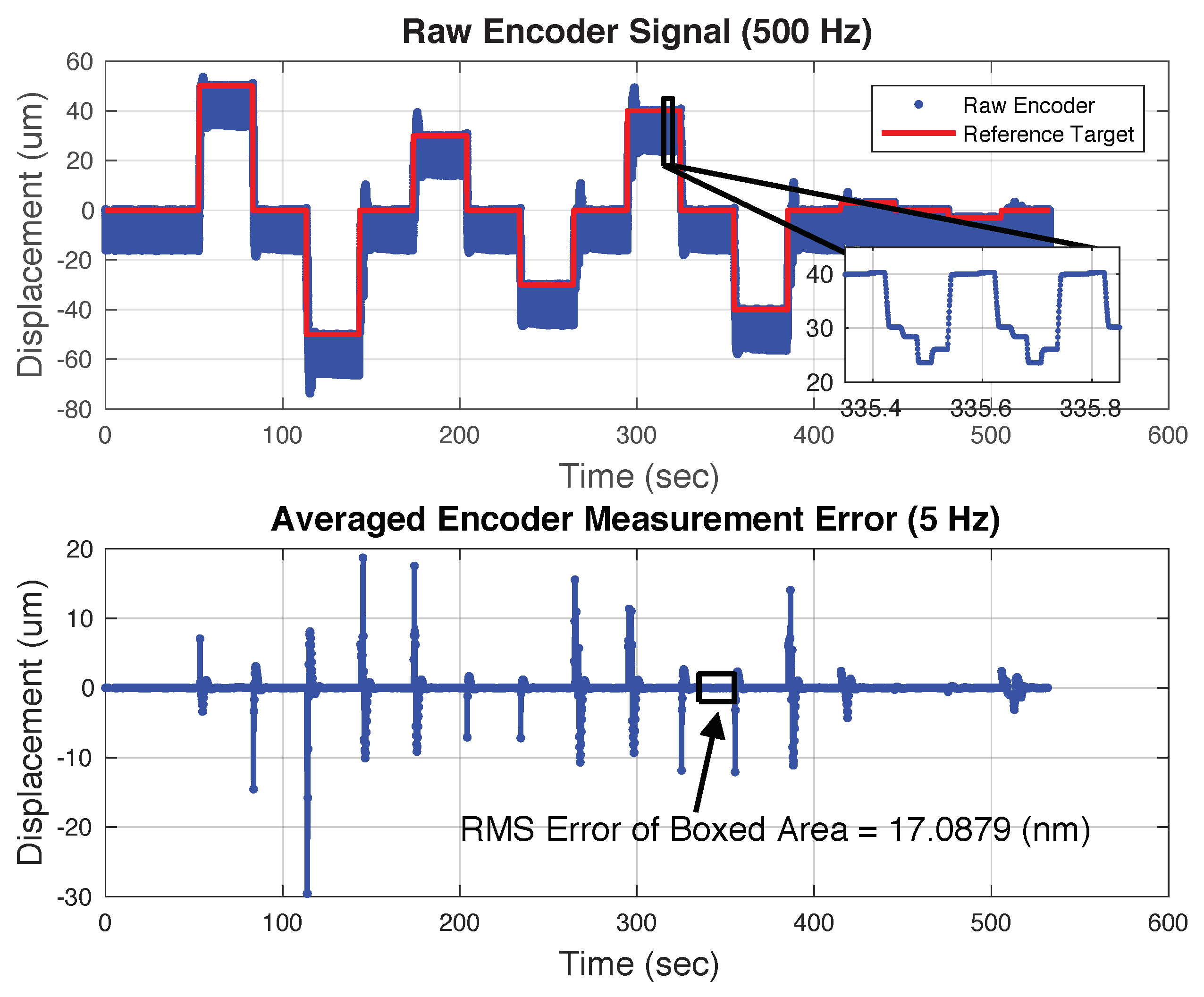
Figure 10 shows the typical encoder and error signal for stepwise moves of the 20-micron FIA. For this test the full control scheme shown in
Figure 4 was employed. The prefilter, feedforward, brake disturbance, and scale factor estimates were all used. During regulation, the RMS error was ∼17 nm which is quite a bit larger than the error for the 6-micron FIA. There are several reasons why the performance of the 20-micron FIA was worse than that of the 6-micron FIA. First among these is the fact that the 20-micron device had a greater variation of the brake disturbance during regulation. Since the control scheme uses measurements from the previous step to predict the brake disturbance during the current step, the larger variation in the brake disturbance would cause larger disturbance prediction errors and larger regulation errors. The exact reason for the large brake disturbance variation is unclear but during this test the environmental spring force was greater than during the testing of the 6-micron device due to the larger position offset during this test. Also of consequence is that the carbide runner hardness may have had a detrimental effect on the brake disturbance as compared to the stainless steel runner. The 20-micron device also had a slenderer aspect ratio which likely made the device more susceptible to transverse loading and buckling. Adding redundant brake PZTs the height of the mechanism grew from 28 mm to 42 mm while the brake wall thickness remained the same.
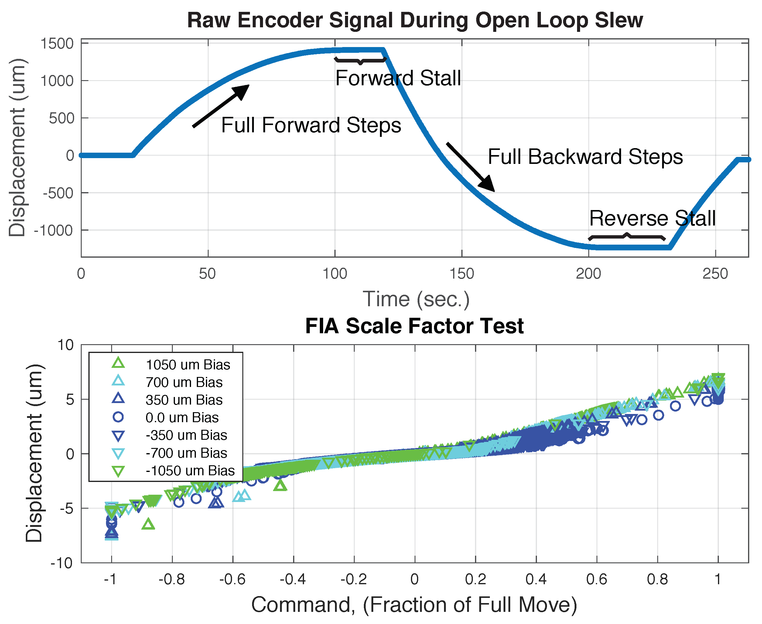
To see how the properties of the mechanism change as the environmental impedance is engaged the 6-micron FIA mechanism was operated with open loop slews and closed loop dithering. This data is shown in
Figure 11. In the top subplot full forward steps were taken until a stall condition was reached and then the steps were reversed, and this process repeated in the opposite direction. The stall condition was reached because the brake disturbance grows as the environmental spring force increases with the displacement. This disturbance motion grows with the environmental spring force until it equals the step displacement at which time an equilibrium of the two displacements is reached. Similar observations were made by [
6,
10].
The stall condition cannot be due to a reduction in the step size as this remains relatively unchanged as shown in the bottom subplot of
Figure 11. This subplot shows closed loop scale factor data during dithering of the closed loop servo about various offset positions. The dither was introduced in software by changing the reference position of the control loop. A dither profile of +20.0, 0.0, −20.0, 0.0, +10.0, 0.0, −10.0, 0.0 microns was used with bias positions of 0.0 microns, ±350.0 microns, ±700.0 microns and ±1050.0 microns. The test jig springs were balanced at the center or 0.0 micron bias position to the level allowed by the residual friction of the open brakes. Although the scale factor does exhibit variation in the full step size due to the different bias positions by itself it is not enough to explain the stall condition, the stall must be due to the increasing brake disturbance. Nonetheless, since both the brake disturbance and scale factor do change this further validates the need for online estimation and compensation of both variables as the actuator is moved about its workspace.
6. Conclusions
The primary difficulty with this actuator technology is the variability of the brake-induced motion of the runner. With control we have been able to compensate for this flaw and achieve nanometer-level positioning over distances of centimeters, a dynamic range of over 120 dB. Further enhancements in performance will likely require improved mechanical design particularly for the 20-micron FIA. One of the key design parameters of these mechanisms seems to be the aspect ratio of the brakes. Based on the results in this paper, the short brakes with thick walls used in the 6-micron device do perform better than the slender brakes used in the 20-micron device (3-micron brake disturbance for the 6-micron FIA and 5 microns for the 20-micron FIA). This is likely due to buckling of the brake as it engages the runner.
Although the FIA mechanisms are designed to hold tens of pounds of load we can expect their positioning performance to degrade at these high force levels. If the runner is subject to large side forces from the environmental spring this leads to larger brake-induced motion. A way of mitigating this brake disturbance is to use a soft environmental spring. This would lessen the force that the brake must hold against and reduce the transverse loading of the brakes.
Geometry changes to the cylindrical runner should also be investigated in terms of reducing the brake disturbance. A square runner, for example, would provide a better friction surface for holding strength and provide additional physical constraints that would prevent buckling of the brake. Runners made of softer materials or texturized surfaces may also provide a more repeatable contact surface. The hardened runners used in the prototype devices were extremely hard making the braking dependent on small surface imperfections which are impossible to avoid.
On the algorithm side, it seems a certain amount of smoothing of the brake disturbance measurements is required. Since encoder noise corrupts the measurement of the brake disturbance, averaging of these measurements is advisable. On the other hand, too much smoothing might not track the faster real variations in the brake disturbance. This is particularly a problem during slews where the brake disturbance varies quite a bit. During steady state regulation the brake disturbance is much more constant allowing for a greater degree of smoothing.
The simulation and testing done in this paper revealed and interesting and unexpected result in that the brake disturbance demonstrated a strong correlation with the extension command. Estimating this functional dependence in the same way we estimated the inverse scale factor may provide some benefits especially during slewing where this dependence comes into play. Using this function to predict the brake disturbance for the next step should improve performance compared to the case of using only past brake disturbance measurements to formulate an estimate. If accurate brake disturbance predictions can be made, then removing the second integrator from the feedback compensator would be useful since this would greatly improve the phase and gain margins of the servo.
Depending on the performance requirements of a particular application the brake disturbance flaw in this inchworm technology should be addressed before successful commercialization or use in a flight project. Two design goals should be emphasized. The first is that the brake disturbance should be a relatively small percentage of the maximum step size, say less than 10%. This is needed to preserve the ability to move bi-directionally. Second, the variation of brake disturbance over time should be minimized. This makes it easier for the software to predict and cancel the brake disturbance.
One criticism of inchworm technology is that the slew rates are somewhat limited. This issue can be addressed by simply increasing the step rate or by increasing the travel range of the extension PZT. The step period is limited only by the response time of the PZTs and associated electronics which can be quite fast. Step rates on the order of 50 Hz instead of the 5 Hz used here should be easily attainable. In addition, the FIA mechanism can be operated in “analog” mode whereby the extension PZT is continuously powered (with the earth brake open and the non-earth brake closed.) to keep position of the runner at some desired reference. This mode would have a much greater bandwidth capability then the stepping mode. To take advantage of this available bandwidth, software could be developed that seamlessly switches between the stepping mode and analog mode as the reference position is approached. There would also have to be a “renormalization” procedure that would be employed when analog mode operation approaches the end of the extension PZT range of motion. This renormalization would have to re-center the extension PZT without moving the runner.
