Abstract
The study of vibration characteristics and suppression methods in integrated electric drive systems of electric vehicles is of critical importance. To investigate these characteristics, both current harmonics within the motor and nonlinear factors within the drivetrain were considered. A 17-degree-of-freedom nonlinear torsional–planar dynamic model was developed, with electromagnetic torque and output speed as coupling terms. The model’s accuracy was experimentally validated, and the system’s dynamic responses were analyzed under different working conditions. To mitigate vibrations caused by torque ripple, a coordinated control strategy was proposed, combining a quasi-proportional multi-resonant (QPMR) controller and a full-frequency harmonic controller (FFHC). The results demonstrate that the proposed strategy effectively suppresses multi-order current harmonics in the driving motor, reduces torque ripple by 45.1%, and enhances transmission stability. In addition, the proposed electromechanical coupling model provides valuable guidance for the analysis of integrated electric drive systems.
1. Introduction
The integrated electric drive system (IEDS) is one of the core components of electric vehicles, widely promoted for its high power density, high efficiency, compact size, and low cost. Its mechanism analysis and application research have attracted increasing attention [1]. The IEDS typically consists of a drive motor, motor controller, and gear transmission system [2], eliminating components such as the longitudinal driveshaft and couplings. A splined structure rigidly connects the motor rotor to the transmission system. Torque ripple from the motor increases dynamic loads in the transmission system, inducing torsional vibrations [3]. The coupling between torsional and planar vibrations further complicates the system’s dynamic behaviors. However, there is still a lack of multi-dimensional electromechanical coupling dynamic models for the IEDS, posing challenges for optimizing its noise, vibration, and harshness (NVH) performance. Therefore, studying the dynamic characteristics of the IEDS with electromechanical coupling and developing suppression strategies for torque ripple is of great significance.
In terms of transmission system dynamics, most scholars focused on the influence of nonlinear excitations such as time-varying meshing stiffness, meshing damping, transmission errors, tooth backlash, bearing stiffness, and bearing damping on system vibration [4,5,6,7,8]. With the increase in degrees of freedom (DOFs), studies have shifted from pure torsional to torsional–planar coupled vibrations. Initial models considered only torsional dynamics to analyze parameter effects on the vibration behavior of the system [9,10]. Hua et al. [11] proposed a transmission system model with 86-DOF based on the Timoshenko beam theory by discretizing the gear shaft and incorporating gear meshing stiffness, meshing damping, and loaded transmission error. The results indicated that gear meshing excitation dominates at higher motor speed. Mo et al. [12] proposed a 16-DOF model of the IEDS, considering bending–torsional–axial–pendular coupling dynamics, and integrated it with the vertical dynamics model of the vehicle. Dong et al. [13] developed a 24-DOF bending–torsional–axial–pendular dynamic model for a double-helical gear transmission system, considering time-varying meshing stiffness, tooth backlash, damping, comprehensive transmission error, and external load excitation. The study focused on the impact of backlash and other factors on the system’s amplitude–frequency response characteristics.
In addition to the internal excitations of the transmission system, the output characteristics of the motor have been identified as major excitation sources. Spatial harmonics arising from motor manufacturing deviations and temporal harmonics resulting from nonlinearities in motor control systems collectively induce superimposed effects on electromagnetic torque. This combined action serves as the primary source of the torque ripple.
Regarding the electromechanical coupling characteristics of the IEDS, Yi et al. [14] developed a mathematical model of a multi-stage electric gear transmission system by considering the motor’s electromagnetic behavior and the gearbox’s torsional–translational vibrations. Electromagnetic torque was used as a coupling variable to analyze system dynamics. Liu et al. [15] proposed a trajectory-based method that reduces system dimensionality while maintaining stability. Through modal analysis, they revealed the relationship between system stability and resonance. Hu et al. [16,17] built an electromechanical coupling dynamic model of the IEDS considering inverter dead-time, voltage drops, and system nonlinearities. They studied the impact of harmonic torque on system performance and dynamic behavior under various conditions and proposed a harmonic torque suppression strategy. Chen et al. [18] focused on a permanent magnet synchronous motor (PMSM) drive system, considering the effect of torsional angle on magnetomotive force, and clarified the relationship between motor structural parameters and torsional vibrations. Fang et al. [19] analyzed the influence of current harmonics on electromagnetic force and the interaction between electromagnetic force harmonics, gearbox behavior, and system vibrations. Results indicated that electromagnetic force and gear meshing force are dominant contributors to system vibrations. Chen et al. [20] proposed a torsional vibration identification method and an active harmonic current injection strategy to suppress vibration, although planar vibrations were not included in the model. Bai et al. [21] investigated the effects of multiple internal excitations and parameters on system dynamics, but did not consider motor harmonics. Fan et al. [22] analyzed the influence of internal excitation on vibration characteristics. The results showed that under variable load or speed conditions, electromagnetic effects caused by electromagnetic stiffness and damping introduced new vibration modes to the system, which may lead to low-frequency torsional vibration. Ge et al. [23] considered nonlinear factors such as stator slotting, pole distribution, and magnetic saturation, and developed an improved equivalent magnetic network model for PMSM under non-stationary conditions. The multi-physical coupling vibration characteristics of the electric drive system were analyzed. The results indicated that electromagnetic damping and stiffness have a certain attenuation effect on the impact experienced by the main and auxiliary gear pairs.
In summary, the driving motor leads to electromagnetic excitation. Torque ripple induced by current harmonics is a major contributor to torsional vibrations. Moreover, the coupling of different vibration modes enriches the dynamic response of the IEDS. Therefore, suppressing harmonic currents is essential for reducing torque ripple and achieving effective vibration mitigation in the system.
Torque ripple suppression (TRS) techniques for PMSMs generally fall into two categories: structure-based design and control strategy-based methods [24]. Structure-based TRS focuses on optimizing motor topology, such as employing skewed slots [25], increasing rotor skew steps [26], designing alternative permanent magnet shapes [27], or changing stator winding configurations [28]. However, these approaches often incur high development costs, offer limited generalizability, and are unsuitable for motors already in service. As a result, control strategy-based TRS methods are more widely adopted [24]. Extracting harmonic currents and feeding them into a PI controller to generate compensation values is a commonly used method for harmonic suppression [29,30]. Some scholars designed improved repetitive controllers to suppress current harmonics caused by the nonlinear characteristics of inverters [31,32]. Zhang et al. [33] proposed a segmented phase-compensated adaptive proportional–integral resonant controller, which reduces computational load and improves system stability while maintaining harmonic suppression performance. Wu et al. [34] proposed a control strategy called quasi-proportional resonant sliding mode control. Based on the combination of current tracking error and the compensation term of the 6th harmonic component, a current error proportional resonant sliding mode control surface is formed to enhance the harmonic suppression capability of the system. Song et al. [35] introduced an ATRS algorithm that combines a fuzzy quasi-proportional–resonant controller with sliding Fourier feedback control, reducing the number of parameters required in practical applications. While PR controllers offer strong harmonic targeting capabilities, they often need to be combined with other controllers to handle multiple harmonic orders effectively. Qian et al. [36] constructed a dq-axis voltage prediction model using the deep belief network (DBN)—deep neural network (DNN) algorithm as the surrogate model, reducing the current harmonic components caused by the harmonic injection structure and PI control algorithm. Li et al. [37] demonstrated that a suppression algorithm based on recurrent neural networks (RNNs) and decision fusion outperforms other methods in reducing the 5th and 7th harmonic currents.
Based on the above analysis and previous research background, it is evident that research integrating multi-dimensional vibration characteristics and suppression methods of the IEDS, considering both motor and transmission system dynamics, is limited. Neglecting electromechanical coupling or focusing solely on torsional vibration fails to accurately reflect the system’s dynamic response, impacting the design of effective vibration reduction strategies.
In order to address this issue, the IEDS mechatronic coupling torsional–plane 17-DOFs dynamic model is established in this paper, incorporating multiple excitation factors, and its dynamic response characteristics under different working conditions are analyzed. At the same time, an active harmonic control strategy is proposed to suppress the system vibration. The main contributions of this paper are listed as follows:
(1) Section 2 presents a multi-DOF electromechanical coupling dynamic model of the electric drive system;
(2) Section 3 validates the model through a bench test and investigates the system’s dynamic behavior under different conditions;
(3) Section 4 proposes a harmonic current control (HCC)-based vibration suppression strategy. Simulation results confirm its effectiveness in suppressing multi-order current harmonics, reducing torque ripple, and improving the system’s NVH performance.
2. Electromechanical Coupling Dynamic Model of the IEDS
2.1. Multi-Directional Coupled Vibration Dynamic Model of the IEDS
The electromechanical coupling model is composed of the dynamic motor model in Section 2.2 and the transmission system dynamics model in Section 2.3. Its coupling principle is shown in Figure 1.
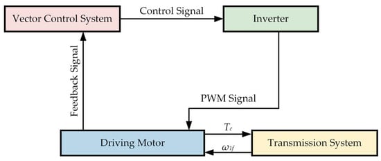
Figure 1.
Schematic diagram of electromechanical coupling for the IEDS.
As shown in Figure 1, the electromagnetic torque and rotational speed of the motor serve as the power input into the transmission system, while the rotational speed feedback of the input shaft is the control object of the motor.
2.2. Decoupling Model of PMSM Considering Nonlinear Factors of the Inverter
The following assumptions are made when establishing the decoupling model:
① Ignore the saturation of the stator and rotor cores of the motor; that is, there is no demagnetization effect in the magnetic circuit.
② In a stable state, the current and voltage waveforms inside the motor are both three-phase sine waves.
③ Ignoring the eddy current loss and hysteresis loss of the motor.
④ The rotor has no damping winding, and the influence of flux linkage harmonics is ignored.
⑤ The self-inductance and mutual inductance of the stator and rotor windings do not change with the current.
2.2.1. Dual-Level Three-Phase Bridge Voltage Source Inverter Model
A typical dual-level three-phase bridge voltage source inverter (VSI) is shown in Figure 2.
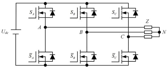
Figure 2.
The structure of the bridge-type voltage source inverter.
In the figure, , , , , , are the six power-type switch elements on the upper and lower bridge arms, respectively. Assuming complementary switching between the upper and lower switches of each phase, the inverter has eight possible switching states. The corresponding basic voltage space vector can be expressed as:
where is the DC bus voltage. The relationship between the three-phase AC voltage, , , and the switching state functions is given by Equation (2) [3].
2.2.2. Decoupling Model of PMSM
The PMSM is a strongly coupled and complex nonlinear system. Model order reduction and variable decoupling are achieved based on coordinate transformation to obtain the motor model in a rotating d-q coordinate system [1]. It can be expressed as:
where and represent the voltages; and represent the currents; and represent the inductances, and represent the magnetic flux linkages; all the above variables are in the d-q coordinate system. is the phase resistance; is the electric angular velocity. The expression of and is:
where is permanent magnet flux linkage. Substituting (4) into Equation (3), the expression for the voltages is as follows:
Similarly, the output torque of PMSM can be expressed as:
In the formula, is the electromagnetic torque and is the number of pole pairs. The relationship between mechanical angular velocity and electrical angular velocity can be described as:
2.2.3. Harmonic Currents Caused by Inverter Nonlinearity
To avoid short circuits in VSI, a fixed dead time is inserted in the sampling period of the pulse width modulation (PWM), resulting in output voltage errors in the inverter. In addition, the presence of a voltage drop in the electronic components in the inverter also generates an output voltage error.
The Fourier decomposition is used to obtain an expression for the output error current in the natural coordinate system, using the phase A current as an example [38]:
where represents the error voltage, and from Equation (8), it is evident that harmonic amplitudes are negatively correlated with harmonic orders. The Y-connection of the three-phase windings cancels out the 3k-order harmonics, leaving 5th, 7th, 11th, 13th, and other orders present within the motor. Based on the principle of coordinate transformation, the expression for error current transforms to Equation (9).
In the formula, the 5th, 7th, 11th, and 13th harmonic components in the three-phase current are transformed to 6th and 12th harmonics in the d-q coordinate system.
2.2.4. Harmonic Currents Caused by Sampling Bias Error
During real-time current sampling, circuit imbalances and zero-point drift in the sensor’s internal components introduce offset current. The offset current in the d-q coordinate system can be described as:
In the formula, and are the bias currents of phase A and phase B, respectively. and are the current sampling errors of phase A and phase B, respectively. The current harmonic orders based on Equations (8)–(10) are summarized in Table 1. The main parameters of the PMSM are shown in Table 2.

Table 1.
Harmonic sources and order distribution of the PMSM.
Table 2.
The main parameters of the PMSM.
2.3. Multi-Directional Coupled Vibration Dynamic Model
Figure 3 shows the architecture of the IEDS. The main reducer adopts a two-stage helical gear set with a parallel-axis layout. The shaft connected to the motor rotor is defined as the input shaft, while the output shaft consists of the half shafts and the differential housing. An intermediate shaft is positioned between and parallel to the input and output shafts. A rigid spline connection is used between the motor shaft and the input shaft of the transmission system. Power is delivered from the drive motor through the input shaft of the main reducer, transmitted via the differential to the left and right half shafts, and finally to the wheels.
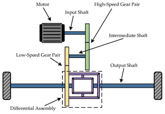
Figure 3.
The architecture of the IEDS.
To accurately characterize the system’s vibration behaviors and investigate the influence of electromechanical coupling, a multi-DOF coupled dynamic model of the IEDS is developed. The model consists of a pure torsional model of the electric drive system and a planar vibration model of the two-stage helical gear–rotor–bearing assembly.
2.3.1. Pure Torsional Vibration Model of the Transmission System
For the pure torsional vibration model that only considers rotational DOFs, the system is discretized using the lumped mass method. In Figure 3, the drive motor, gears, wheels, and vehicle body are simplified as mass elements with rotational inertia only. Shaft components are modeled as elastic elements, considering only torsional stiffness and damping, represented in a parallel “spring-damper” configuration, as shown in Figure 4. The low-speed driven gear and the differential shell are bolted together and simplified as a differential assembly.
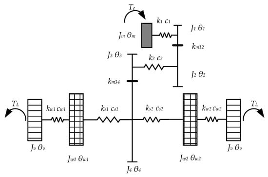
Figure 4.
Simplified diagram of pure torsional vibration for the IEDS.
Based on Newton’s second law, an 8-DOF pure torsional vibration model of the IEDS is established, as shown in Equation (11).
In the formula, , , , , , , , and represent the equivalent moment of inertia of the motor rotor, high-speed driving gear, high-speed driven gear, low-speed driving gear, differential assembly, left wheel, right wheel, and vehicle body, respectively. , , , , , , , represent the motor rotor, high-speed driving gear, high-speed driven gear, low-speed driving gear, differential assembly, left wheel, right wheel rotational angle, and vehicle body equivalent rotational angle, respectively. Correspondingly, , , , , , , , are their angular velocities. The equivalent torsional stiffness and damping of the input shaft, intermediate shaft, left half-shaft, right half-shaft, left wheel, and right wheel are denoted by , , , , , and , , , , , , respectively. is the external load. Parameter values are listed in Table 3 and Table 4.
Table 3.
Equivalent moment of inertia of components.
Table 4.
Torsional stiffness and torsional damping of the components.
2.3.2. Planar Vibration Model of Two-Stage Helical Gear–Rotor–Bearing System
The meshing displacement of the gear pair affects the torsional vibration of the gears, leading to variations in the dynamic meshing force. These variations, in turn, induce planar vibration of the gears. Therefore, a coupling effect exists between the two vibration behaviors within the system.
During the gear meshing process, the main nonlinear excitation factors considered are time-varying meshing stiffness, meshing error, and tooth side clearance [14]. When the contact ratio is large, the change of the dynamic meshing stiffness of the gear approaches a sine wave. The frequency of the waveform change is the gear meshing frequency, and the meshing stiffness and meshing frequency can be calculated as:
where represents the average value of the comprehensive meshing stiffness; S denotes the amplitude ratio, set to 0.4 in this paper. φ is the phase angle, z is the number of teeth, and is the rotational frequency.
The meshing damping coefficient is assumed to be a constant of 0.1, leading to the expression for meshing damping as follows:
In the formula, is the radius of the base circle of the gear, and is its equivalent rotational inertia, with subscript i = p and g representing the driving and driven gears, respectively. The expression for the meshing error is given by:
where is the constant term of the transmission error, set to 0 in this paper, is the amplitude of the static transmission error, and is the initial meshing phase angle.
To ensure proper meshing of the gear pair under various operating conditions, a certain backlash is maintained between the driving and driven gears during assembly. This tooth backlash is characterized by the equivalent gear backlash function :
where b is half the tooth backlash. Considering these nonlinear factors, the dynamic meshing force can be expressed as:
where is the meshing contact line displacement. Additionally, in this paper’s IEDS, a fixed installation angle is considered, as shown in Figure 5.
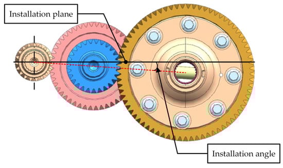
Figure 5.
Diagram of the installation angle of the IEDS.
Therefore, the relative displacement at the gear meshing point can be calculated by Equation (17):
In the formula, and are the rotation angles of the driving and driven gears, and are the displacements along the x direction of the driving and driven gears; and are the displacements along the y direction of the driving and driven gears; and are the displacements along the z direction of the driving and driven gears, and is a base circle helix angle.
In the helical gear meshing model, is decomposed, respectively, along three directions; the axial force , radial force , and tangential force can be expressed as:
where denotes the italic pressure angle at the gear meshing point, represents the helix angle at the reference circle, and refers to the working pressure angle at the gear end face.
The tangential force generates the meshing torque in the gear pair, as obtained from Equation (19):
where and (i = 1, 2, 3, 4) represent the meshing torque and the reference circle radius of the gear, respectively. The subscript i corresponds to the high-speed driving gear, high-speed driven gear, low-speed driving gear, and low-speed driven gear, in sequence.
According to Equation (18), gear meshing force induces vibrations in three orthogonal planes, resulting in variations in meshing forces. Neglecting shaft deflection and relative displacements between shaft-mounted components and the shafts, three sets of deep groove ball bearings are modeled using equivalent stiffness and damping elements to simulate dynamic bearing forces. A planar vibration model of the gear pairs is established, as illustrated in Figure 6.
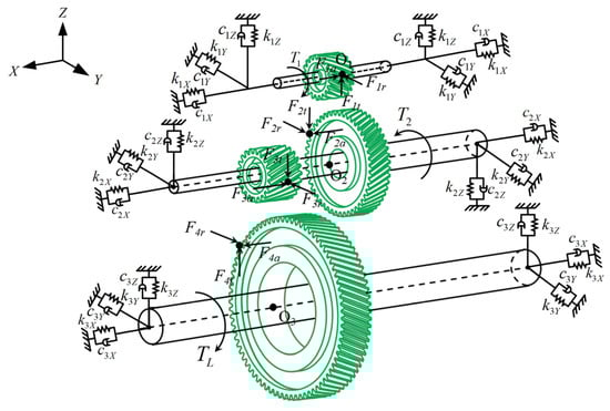
Figure 6.
Planar vibration model of the gear–rotor–bearing system.
In Figure 6, , , and represent the centroids of the input shaft, intermediate shaft, and output shaft, respectively, considering the mass of shaft-mounted components. The subscripts 1, 2, and 3 indicate the order of power transmission. A 9-DOFs planar vibration model of the gear–rotor–bearing system can be described as:
In the formula, (i = 1, 2, 3) correspond to the effective masses of the shafts, considering the attached gears; , , and (i= 1, 2, 3) denote the relative displacements of the shaft centroids along the x, y, and z directions, respectively; (i = 1, 2, 3, 4; j = a, r, t) represent the axial, radial, and tangential forces acting on the gears, respectively. , , and (i = 1, 2, 3) are the three-directional support stiffnesses of the bearing, while , , and (i = 1, 2, 3) are the corresponding support dampings. The parameters of the gear pairs and the deep groove ball bearings are listed in Table 5 and Table 6 and Table 7, respectively.
Table 5.
Structural parameters of two-stage helical gear pairs.
Table 6.
Meshing parameters of two-stage helical gear pairs.
Table 7.
Structural parameters of deep groove ball bearing.
By integrating the two sets of vibration equations from Equations (11) and (20), a complete 17-DOFs multi-directional coupled dynamic model of the IEDS is established. Since gears are fixed to shafts, gear displacements are assumed to be consistent with shaft displacements. During operation, shaft displacements are transmitted to bearings at both ends, causing variations in bearing forces that act as excitations. These bearing excitations, in turn, affect the planar vibration of the shaft system, altering the gear meshing displacement and consequently influencing the torsional vibration behaviors of the system.
3. Model Verification and Dynamic Responses Analysis
3.1. Model Verification
To identify the key sources of vibration and noise in electric vehicles, current research commonly employs methods such as acceleration response measurement [39], sound pressure level testing [40], spectrum analysis [41], and order tracking analysis [42]. Among these, spectrum analysis is widely used in the IEDS due to its high-resolution capability in distinguishing structural and electromagnetic excitations under steady-state working conditions. This method enables the extraction of signal components at different frequencies, directly revealing frequency peaks caused by specific excitations, and provides important guidance for NVH performance optimization.
In this study, spectrum analysis is adopted. The experimental test bench and instrumentation layout are shown in Figure 7 and Figure 8, respectively.
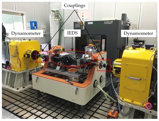
Figure 7.
The test bench of the IEDS.
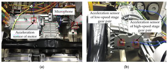
Figure 8.
Component arrangement for testing: (a) top view; (b) side view.
As illustrated in Figure 7, the test bench consists of the IEDS, couplings, dynamometers, and others. Couplings connect the left and right half-shafts to the dynamometers, which provide the load for the system.
Prior to testing, a calibrator is used to determine the noise measurement range. The microphone is positioned 1 m away from the integrated powertrain. Three tri-axial acceleration sensors are mounted at the motor and at the two-stage driving gears on the main reducer housing, as shown in Figure 8.
The data acquisition frontend is supplied by Siemens (Siemens Industry Software NV, Leuven, Belgium), and post-processing is performed using Siemens LMS Test. Lab software (Version 2021.1, developed by Siemens Industry Software NV, Leuven, Belgium.). This software uses order extraction techniques tailored for rotating machinery to identify significant orders of vibration and noise amplitude, as well as the associated mechanical components. Under steady-state conditions with constant speed, target components can be directly identified based on characteristic frequencies, which remain constant regardless of the type of signal collected. Vibration signals are converted into noise signals via a transducer and then imported into the post-processing software.
Based on the above methodology, characteristic frequencies are used as validation indicators to evaluate the effectiveness of the dynamic model. The test condition corresponds to a vehicle speed of 15 , with a driving motor speed of 1000 and an electromagnetic torque of 10 , lasting for 6.5 s. The theoretical values of the fundamental frequency of current harmonics excitation, high/low speed stage gear meshing excitation for this condition are 66.67 Hz, 316.67 Hz, and 183 Hz, respectively, which are denoted as , , and , in that order. Meanwhile, using the term (n = 1, 2, 3…) denotes the multiple frequencies of the corresponding excitation. The resulting noise waterfall plot of the IEDS is shown in Figure 9.
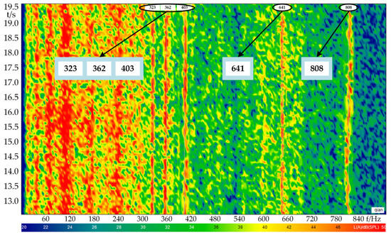
Figure 9.
Overall noise waterfall diagram of the IEDS.
In Figure 9, the x-axis represents sound pressure level and frequency components, and the y-axis indicates test duration. Red zones represent noise levels exceeding 50 dB. Characteristic frequency components include 323 Hz, 362 Hz, 403 Hz, 641 Hz, and 808 Hz, corresponding to , , , , and , respectively. These results indicate that the primary sources of the system’s vibration and noise are gear meshing excitation and current harmonics excitation, consistent with theoretical analysis. The error distribution between the theoretical and experimental values of characteristic frequencies is shown in Table 8.
Table 8.
Error distribution of characteristic frequencies.
3.2. System Dynamic Response Analysis
3.2.1. Steady-State Condition
According to previous studies, the IEDS is prone to resonance in the low-frequency band, and the vibration and noise inside the vehicle are larger when traveling at low speed. Therefore, the simulation speed is 15 (motor speed is 1000 ), the load torque of the transmission system is 70 (motor torque is 10 ), and the simulation condition is set up, which is recorded as Condition 1. The time- and frequency-domain characteristics of the electromagnetic torque as a coupling term are shown in Figure 10.
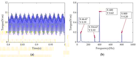
Figure 10.
Time- and frequency-domain analysis of electromagnetic torque : (a) time-domain; (b) frequency-domain.
As shown in Figure 10, the electromagnetic torque ripples within around its expected value. The dominant excitations affecting the fluctuation are , , , and .
The angular acceleration of components not only reflects the dynamic behavior of rotating machinery but also establishes a link with force/torque, making it a key indicator for evaluating torsional vibration. Figure 11 presents the time- and frequency-domain responses of angular acceleration for the motor rotor, high-speed driving/driven gear, low-speed driving gear, and the differential assembly.
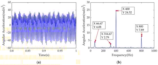
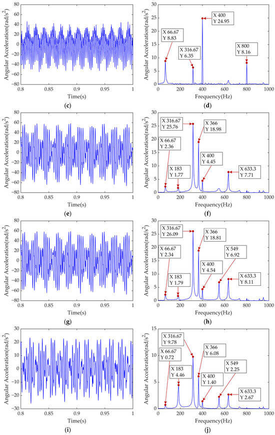
Figure 11.
Time- and frequency-domain analysis of torsional vibration dynamic responses of components of the IEDS: (a) time-domain of ; (b) frequency-domain of ; (c) time-domain of ; (d) frequency-domain of ; (e) time-domain of ; (f) frequency-domain of ; (g) time-domain of ; (h) frequency-domain of ; (i) time-domain of ; (j) frequency-domain of .
A comparison of Figure 11a,c,e,g,i reveals that components on the same shaft exhibit similar torsional vibration characteristics. The high-speed driven gear and low-speed driving gear show the largest vibration amplitudes, primarily due to the presence of two gear pairs on the intermediate shaft, where the superposition of meshing effects amplifies the vibration. In contrast, the differential assembly, located at the output shaft, operates at lower rotational speeds and has the largest rotational inertia after two-stage helical gear reduction, resulting in the smallest torsional vibration amplitude.
In the frequency-domain responses shown in Figure 11b,d, the dominant excitation components for the motor rotor and high-speed driving gear are , , and , with being secondary. As the torque is transmitted through the gear pairs, the vibration induced by current harmonics gradually decreases, while that caused by gear meshing forces increases. In Figure 11f,h,j, the high-speed driven gear on the intermediate shaft is mainly excited by the meshing fundamental frequencies and , along with their harmonics and . Excitations from and are weakened. The low-speed driving gear and differential assembly additionally show a excitation.
Based on the above analysis, all components are influenced by both current harmonics and gear meshing forces to varying degrees. The meshing forces from high-speed gear pairs induce greater vibration amplitudes than those from low-speed pairs.
To evaluate the gear meshing condition, the time- and frequency-domain responses of the dynamic meshing forces for the two-stage helical gear pairs are shown in Figure 12.
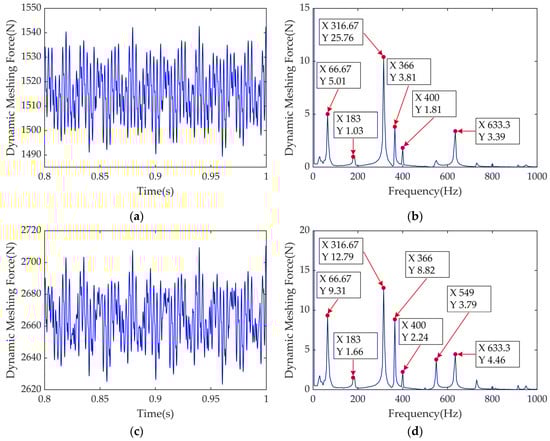
Figure 12.
Time- and frequency-domain analysis of dynamic meshing force of high-speed gear pairs and low-speed gear pairs : (a) time-domain of ; (b) frequency-domain of ; (c) time-domain of ; (d) frequency-domain of .
As illustrated in Figure 12, the meshing force of the high-speed gear pair is smaller than that of the low-speed gear pair. The calculated average for the former is 1515.8 N, with a maximum amplitude range of 53.4 N. While for the latter, the average is approximately 2664.8 N, with a maximum amplitude range of 87.1 N. In the frequency-domain response, the dominant excitation components affecting both gear stages are and . This is because the motor rotor and high-speed driving gear share the input shaft, which has a significantly lower torsional stiffness than the intermediate shaft. Consequently, excitations on the input shaft have a greater impact on torsional vibrations. Moreover, due to the high meshing stiffness of the gear pairs, the influence of meshing harmonics on the meshing force exceeds that of current harmonics.
3.2.2. Shock Working Condition
When the road is uneven or the vehicle crosses an obstacle, the wheel-end load torque becomes an impact load. To analyze the system’s vibration behavior under these conditions, the motor speed is kept constant while an impact load is applied at 0.5 s. The load torque at the motor output rises from 10 N·m to 30 N·m and then restores the original value, lasting for 0.1 s, recorded as Condition 2. The electromagnetic torque and the torsional vibration responses of components on the input, intermediate, and output shafts are shown in Figure 13.
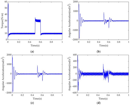
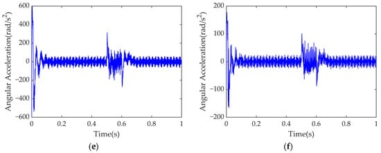
Figure 13.
Time-domain analysis of electromagnetic torque and torsional vibration dynamic responses of components of the IEDS: (a) electromagnetic torque; (b) ; (c) ; (d) ; (e) ; (f) .
In Figure 13, the torsional vibration of components on all shafts intensifies to varying degrees during motor load fluctuations, with components on the same shaft showing similar vibration amplitudes. Since the motor is directly connected to the reducer, Figure 13b,c indicate that the motor rotor and high-speed driving gear exhibit the most severe vibrations, suggesting that load changes have a greater effect on the components of the input shaft.
3.2.3. Plane Vibration Analysis of Shaft System and Solution of Dynamic Bearing Force
To analyze the planar vibration of the IEDS, the vibration displacements of the parallel shaft system in the x, y, and z directions are evaluated, as shown in Figure 14.
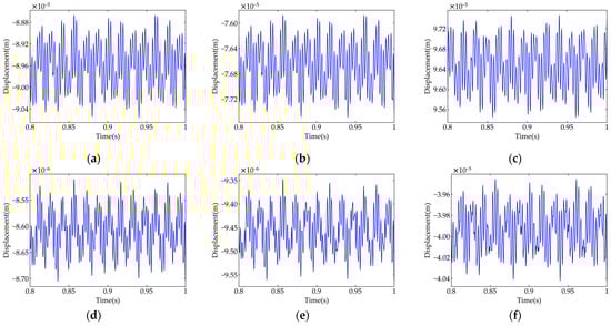
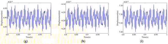
Figure 14.
Three-directional planar vibration response of the shafts: (a) ; (b) ; (c) ; (d) ; (e) ; (f) ; (g) ; (h) ; (i) .
As shown in Figure 14, for the three-directional displacements of each shaft segment, the maximum planar vibration consistently occurs in the z-direction (tangential). With power transmission through two gear pairs and increasing bearing stiffness, displacements in all three directions decrease progressively from the input shaft to the output shaft.
For parallel-shaft helical gear reducers, the vibration characteristics of gears and bearings are highly similar in both the time- and frequency-domain [43]. In this paper, the relative motion between the gear and its mounting shaft is neglected, allowing shaft displacement to represent both gear and bearing displacement. The dynamic bearing force, which influences planar vibration, is expressed as:
where and (i = 1, 2, 3; j = x, y, z) denote bearing stiffness and damping, and , are generalized displacement and velocity, respectively. The three-directional dynamic bearing forces for each shaft are shown in Figure 15.
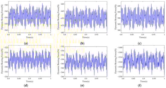
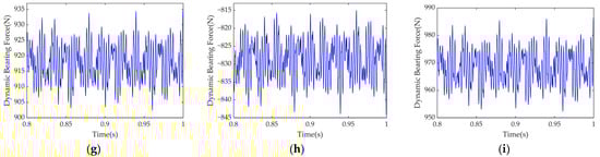
Figure 15.
Response of three-directional dynamic bearing forces: (a) ; (b) ; (c) ; (d) ; (e) ; (f) ; (g) ; (h) ; (i) .
Figure 15 indicates that all shafts exhibit the same trend: the bearing force is largest in the z-direction, consistent with the observed planar vibration. The z-direction (tangential) aligns with the resultant torque and is associated with torsional vibration, confirming the coupling between torsional and planar vibrations. Therefore, both vibration modes should be analyzed concurrently.
4. Active Vibration Suppression Strategy Based on Harmonic Current Controller
To suppress vibration in the IEDS, this paper aims to reduce torque ripple by considering the electromechanical coupling. Previous researchers have mainly focused on injecting a single-order harmonic current to improve the sinusoidal quality of the phase current [44]. However, according to Section 3, harmonic orders that contribute to torque ripple are not unique. Thus, injecting only a single-order harmonic current is insufficient to eliminate torque ripple effectively. This paper proposes an HCC strategy for the driving motor, which combines a quasi-proportional multi-resonant controller with a full-frequency harmonic controller, enabling tracking control of multiple harmonic orders.
4.1. Controller Design
4.1.1. Quasi-Proportional Multi-Resonant Controller
In the d-q coordinate system, all harmonic components appear as AC signals. However, Pl controllers can only achieve zero steady-state error tracking for DC signals. Therefore, harmonic components must be converted to DC values through coordinate transformations and low-pass filtering, which introduces computational complexity and time delays.
The proportional resonant (PR) controller provides infinite gain at a specific frequency for both positive and negative sequences, enabling effective tracking of AC signals. The transfer function of a PR controller can be expressed as [34]:
where , , and are the proportional gain, resonant gain, and resonant frequency, respectively. In Equation (22), the PR controller offers infinite gain at . However, due to limited bandwidth, its harmonic suppression performance degrades significantly when signal frequencies fluctuate. To address this, a first-order low-pass filter is used to replace the integrator, resulting in the quasi-proportional resonant (QPR) controller:
where is the cutoff frequency of the low-pass filter. Since , the higher-order terms containing can be neglected, Equation (23) is simplified to:
To suppress dominant 6th and 12th order harmonics, a quasi-proportional multi-resonant (QPMR) controller is designed. When applied to harmonic current control, the resonant frequency is set to match the corresponding harmonic frequency. The structure of the QPMR controller is shown in Figure 16.
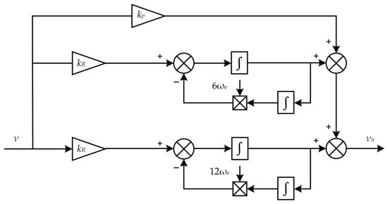
Figure 16.
Structural schematic diagram of the QPMR controller.
Its Bode diagram is shown in Figure 17.
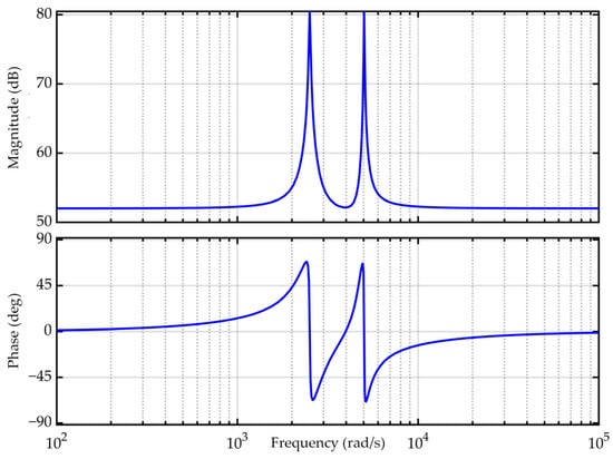
Figure 17.
The Bode diagram of the QPMR controller.
According to Figure 16 and Figure 17, it can be known that the integration parameters of the sub-controller are the same and share the proportional link. This not only avoids multiple parameter tuning but also ensures that the QPMR controller has a large gain at multiple resonant frequencies, thereby suppressing multiple resonant frequencies existing in the system. In this paper, the values of and are set to 400 and 10,000, respectively.
4.1.2. Full-Frequency Harmonic Controller
Beyond the harmonic orders addressed in Section 4.1.1, the QPMR controller is unable to effectively track other harmonics, such as the fundamental (1st order). These untracked harmonics also contribute significantly to torque ripple when accumulated. To address this issue, a full-frequency harmonic controller (FFHC) is proposed to uniformly suppress current harmonics across all orders. The FFHC comprises two components: a harmonic current observer and a harmonic voltage controller. Harmonic currents are extracted using an improved average current method and fed into a fuzzy-PI-based harmonic voltage controller to generate compensation voltage. The control structure is illustrated in Figure 18.
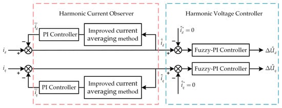
Figure 18.
Structure diagram of the full-frequency harmonic controller.
Common harmonic current extraction methods include the low-pass filter (LPF) method and the current averaging method. The LPF method relies on the cutoff frequency of the filter, while the averaging method utilizes the principle that the integral of a sinusoidal AC signal over one period is zero. To improve accuracy and robustness, an improved averaging method is proposed.
In the d-q coordinate system, the fundamental component of the phase current appears as a DC signal, while harmonics are AC. Harmonic currents cannot be directly isolated using a single coordinate transformation. Therefore, this paper introduces an improved current averaging method that first extracts the fundamental component in the d-q axes. The harmonic content is then obtained by subtracting this fundamental component from the original phase current in each axis. The resulting difference represents the total harmonic content on each axis.
In Figure 18, and represent the average fundamental components of the d- and q-axis currents, calculated as:
where t represents any time instant, T is the fundamental period, and denotes the accumulated current over one fundamental period. The expression for calculating T is:
where n is the rotational speed. The total observed d- and q-axis harmonic currents, denoted as and can be expressed as:
Setting the control targets as and , a fuzzy-Pl compound controller is used to obtain the harmonic voltage compensation terms and .
As shown in Figure 18, fuzzy controller inputs are defined as the error between the target and actual harmonic currents on the d- and q-axes and their changing rate . The output is the harmonic compensation voltage . The basic universes of discourse are defined as , , and , respectively. Assume the intervals of the domains of the fuzzy subsets , , and are , , and , respectively. The quantization factors , and scale factor can be expressed as:
The input and output variables are represented using linguistic terms {NL, NM, NS, ZO, PS, PM, PL}, corresponding to {Large Negative, Medium Negative, Small Negative, Zero, Small Positive, Medium Positive, Large Positive}. Fuzzy control rules are formulated in the structure ”.
For instance, when both and are large negative numbers (NL), indicating a significant and increasing deviation, a large positive value (PL) is assigned to . While is NL and is a large positive number (PL), the deviation is large but decreasing, and is set to a small positive value (PS). This rule design is intended to avoid excessive control actions and to ensure system stability.
Triangular membership functions are used in this design. The control rules are presented in Table 9.
Table 9.
Fuzzy control rules of harmonic compensation voltage.
The fuzzy outputs are derived using the Mamdani max–min inference method, and defuzzification is performed based on the weighted average method. The corresponding expression is given as follows:
In the formula, u denotes the de-fuzzy output value, represents a possible output value, and indicates the degree of membership of in the fuzzy control set.
To address the limitations of fuzzy controllers in eliminating steady-state error and achieving high control accuracy, a fuzzy-PI composite control strategy is adopted. By combining the PI controller with the fuzzy controller, steady-state error can be effectively eliminated and control performance improved through PI control, while robustness and response speed are enhanced through fuzzy control.
Furthermore, an adaptive adjustment factor is introduced to dynamically adjust the weight ratio between the two control strategies in real time, based on the variation of the harmonic current error . When is large, it increases the weight of fuzzy control; conversely, it increases the weight of PI control. The sum of the two weights remains constant at 1. The adaptive adjustment factor can be expressed as:
The compensation voltage of the composite control can be calculated by:
where represents the output voltage of the PI controller, denotes the output voltage of the fuzzy controller. K is a positive constant, and ranges within . According to Equation (30), is negatively correlated with .
In this paper, the domain of the harmonic current error in the d- and q-axes is set to [−15, 15], and the domain of changing rate is [−2000, 2000]. The domain of the harmonic voltage compensation is [−10, 10]. The parameter K of the adaptive adjustment factor is set to 0.9 and 1.26 for the d- and q-axes, respectively.
4.1.3. Harmonic Current Control Strategy for the IEDS
In the driving motor, the QPMR controller is connected in parallel with the PI controller of the motor current loop. Based on real-time sampling, the d- and q-axis currents are used to calculate the harmonic compensation voltage through FFHC, which is then injected into the control system. This approach effectively suppresses current harmonics, reduces torque ripple, and ensures a certain level of system robustness. The principle of coordinated control is illustrated in Figure 19.
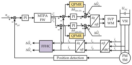
Figure 19.
Current harmonic suppression strategy of the driving motor.
4.2. Simulation Verification of Active Vibration Suppression
4.2.1. Condition 1 Verification
The time- and frequency-domain responses of the electromagnetic torque before and after adopting HCC are shown in Figure 20.
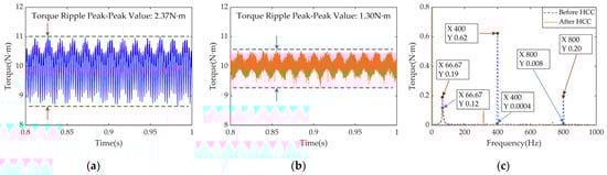
Figure 20.
Time- and frequency-domain comparisons of electromagnetic torque before and after HCC: (a) time-domain before HCC; (b) time-domain after HCC; (c) frequency-domain comparison.
Figure 20a,b compare the time-domain responses of the electromagnetic torque. The average torque remains unaffected by the control strategy, while the peak-to-peak torque ripple decreases from 2.37 N·m to 1.30 N·m after harmonic current injection, that is 45.1%. Figure 20c shows that the frequency-domain components at , , and are significantly attenuated.
Figure 21 illustrates the time- and frequency-domain responses of the d- and q-axis currents before and after HCC.
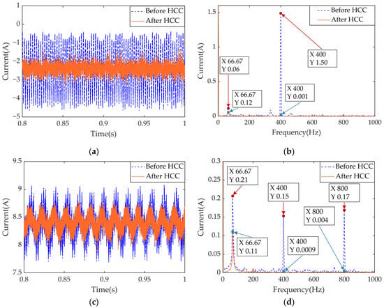
Figure 21.
Comparison of the time- and frequency-domains of the d-axis current and q-axis current before and after HCC: (a) time-domain of ; (b) frequency-domain of ; (c) time-domain of ; (d) frequency-domain of .
As shown in Figure 21a,c, the ripple amplitudes of both d- and q-axis currents decrease after adopting HCC, with a more noticeable reduction on the d-axis. Figure 21b,d reveal that the 6th harmonic component dominates the d-axis current ripple, while the q-axis current is influenced by the 1st, 6th, and 12th harmonics. After adopting HCC, the 6th and 12th harmonics are effectively suppressed in both axes, along with the 1st harmonic. Due to the QPMR controller’s targeted suppression of the and excitations, the coordinated control shows better attenuation effects for these frequencies than for .
Torque ripple caused by current harmonics can induce torsional vibration in the drivetrain. Based on previous analysis, the angular accelerations of key components—the high-speed driving gear, low-speed driving gear, and differential assembly—are selected as indicators of torsional vibration. Additionally, gear meshing torque is considered, as it also contributes to system vibration. The dynamic responses of torsional vibration and gear meshing forces before and after HCC are presented in Figure 22.
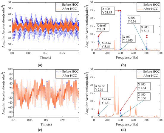
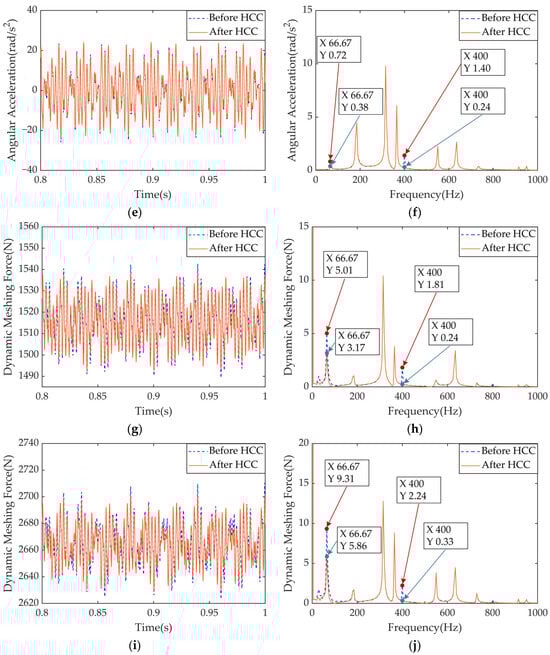
Figure 22.
Time- and frequency-domain comparison of torsional vibration dynamic responses of representative components of the IEDS and meshing force of two-stage gear pairs before and after HCC: (a) time-domain of ; (b) frequency-domain of ; (c) time-domain of ; (d) frequency-domain of ; (e) time-domain of ; (f) frequency-domain of ; (g) time-domain of ; (h) frequency-domain of ; (i) time-domain of ; (j) frequency-domain of .
In Figure 22a,c,e, angular acceleration fluctuations are reduced across all components after HCC. The high-speed driving gear shows the most significant improvement due to its direct connection with the motor rotor, making it more sensitive to torque ripple. Frequency-domain analysis in Figure 22b,d,f indicate effective suppression of excitation components at , , and . Figure 22g,i show that the fluctuation of the meshing force of two-stage gears has also decreased to a certain extent, while Figure 22h,j confirm that harmonic components in the meshing forces are significantly attenuated. These results demonstrate smoother gear transmission and improved drivetrain stability following HCC implementation. The RMSE of the above variables after adopting HCC are presented in Table 10.
Table 10.
RMSE results for variables under Condition 1.
4.2.2. Condition 2 Verification
To evaluate the effectiveness of the coordinated control strategy under impact conditions, the variations in the electromagnetic torque, d- and q-axis currents, and torsional vibrations of key system components before and after implementing HCC are analyzed, as illustrated in Figure 23 and Figure 24.
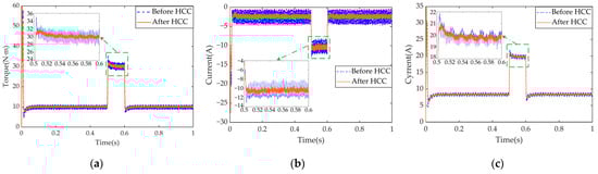
Figure 23.
Time-domain comparison of electromagnetic torque , the d-axis current , and q-axis current before and after HCC: (a) ; (b) ; (c) .
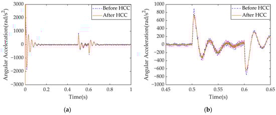
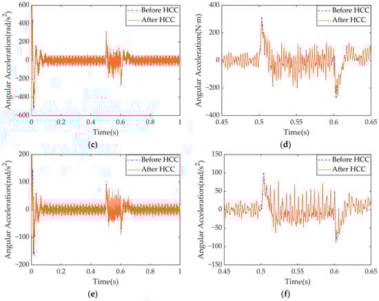
Figure 24.
Comparison of torsional vibration time-domain responses of key components of the IEDS before and after HCC: (a) the overall response of ; (b) response of within the action of shock loading; (c) the overall response of ; (d) response of within the action of shock loading; (e) the overall response of ; (f) response of within the action of shock loading.
As shown in Figure 23 and Figure 24, when the load changes, the HCC strategy effectively suppresses harmonic currents in a timely manner, resulting in reduced peak overshoots in the d- and q-axis currents and decreased torque ripple. This allows the system to transition to a steady-state more smoothly. Furthermore, following a load disturbance, the HCC strategy demonstrates strong robustness by rapidly tracking and suppressing the torsional vibrations of various components, thereby reducing the peak torsional response induced by load transients. The RMSE of the above variables after adopting HCC are presented in Table 11.
Table 11.
RMSE results for variables under Condition 2.
4.2.3. Dynamic Bearing Force Verification
According to the analysis in Section 3.2.3, the shaft system exhibits the largest planar vibration displacement in the z-direction (tangential), which corresponds to the maximum dynamic bearing force in the same direction. The two share a similar trend, indicating that planar vibrations are reflected in the bearing forces. Therefore, the z-direction bearing forces of the three shafts before and after applying HCC are analyzed, as shown in Figure 25.
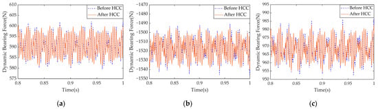
Figure 25.
Comparison of the z-direction dynamic bearing forces of each shaft before and after HCC: (a) input shaft; (b) intermediate shaft; (c) output shaft.
Figure 25 shows that while the HCC strategy does not alter the average bearing force, it significantly reduces the fluctuation amplitude. This implies that harmonic current suppression can effectively mitigate impact loads on the bearings. The RMSE of dynamic bearing force after adopting HCC are presented in Table 12.
Table 12.
Dynamic bearing force RMSE in simulation.
5. Conclusions
In this study, to accurately analyze the vibration characteristics of an integrated electric drive system, a torsional–planar dynamic model was developed that accounts for multiple excitation sources. The model’s accuracy was experimentally validated and used to analyze the system’s dynamic responses under various operating conditions. A coordinated control strategy was proposed to suppress current harmonics and reduce torque ripple.
(1) A mathematical model of a PMSM was established, incorporating inverter nonlinearities and current bias errors. Additionally, a 17-degree-of-freedom bending–torsional–axial coupled vibration model of the integrated electric drive system was constructed, considering various nonlinearities such as time-varying gear mesh stiffness, gear backlash, and meshing errors. The model achieved a validation accuracy of up to 98%.
(2) The dynamic responses under both steady-state and impact conditions were analyzed. It was demonstrated that both current harmonic excitation and gear meshing excitation coexist in the system’s internal variable responses. Furthermore, the interaction between axial z-direction vibration and gear meshing torque indicates a coupling relationship between torsional and planar vibration.
(3) The proposed coordinated control strategy exhibits strong robustness and effectively suppresses 1st, 6th, and 12th order harmonic currents. It reduces torque ripple by 45.1%, mitigates bearing impact loads, and achieves vibration reduction and improved transmission stability for the system.
(4) For practical application in vehicle platforms, factors such as real-time computational load, sensor deployment, and system integration need to be further considered. Although the proposed control strategy shows promising performance, its implementation may pose challenges related to hardware cost and compatibility with existing vehicle control architectures. Further validation on a full vehicle test platform is suggested to assess its effectiveness under realistic operating conditions.
Author Contributions
Conceptualization, Y.C. and H.L.; methodology, Y.C.; software, Y.C. and Y.Z.; validation, Y.C., J.X., and L.Z.; formal analysis, Y.C. and J.X.; investigation, H.L.; data curation, H.L. and J.X.; writing—original draft preparation, Y.C. and H.L.; writing—review and editing, Y.C. and J.X.; visualization, Y.C. and J.X.; supervision, H.L. and Y.Z.; project administration, H.L. and J.X.; funding acquisition, H.L. and J.X. All authors have read and agreed to the published version of the manuscript.
Funding
This research was partially funded by the Guangxi Science and Technology Major Project. Project Name: Research and Application of Key Technologies for Multifunctional Super-Module Integrated Electric Drive System, Project Number: 202401gx0085.
Data Availability Statement
The data is unavailable due to privacy or ethical restrictions.
Acknowledgments
The authors would like to express their gratitude for the useful comments and constructive suggestions from the editor and anonymous reviewers.
Conflicts of Interest
The authors declare no conflicts of interest.
References
- Hu, J.; Guo, Q.; Sun, Z.; Yang, D. Study on low-frequency torsional vibration suppression of integrated electric drive system considering nonlinear factors. Energy 2023, 284, 129251. [Google Scholar] [CrossRef]
- Singirikonda, S.; Pedda, O. Investigation on performance evaluation of electric vehicle batteries under different drive cycles. J. Energy Storage 2023, 63, 106966. [Google Scholar] [CrossRef]
- Chen, S.; Hu, M. Active torsional vibration suppression of integrated electric drive system based on optimal harmonic current instruction analytic calculation method. Mech. Mach. Theory 2023, 180, 105136. [Google Scholar] [CrossRef]
- Chen, Z.; Zhai, W.; Wang, K. Vibration feature evolution of locomotive with tooth root crack propagation of gear transmission system. Mech. Syst. Signal Proc. 2019, 115, 29–44. [Google Scholar] [CrossRef]
- Cai, Z.; Lin, C. Dynamic model and analysis of nonlinear vibration characteristic of a curve-face gear drive. Stroj. Vestn. J. Mech. Eng. 2017, 63, 161–170. [Google Scholar] [CrossRef]
- Mo, S.; Zhang, Y.; Song, Y.; Song, W.; Huang, Y. Nonlinear vibration and primary resonance analysis of non-orthogonal face gear-rotor-bearing system. Nonlinear Dyn. 2022, 108, 3367–3389. [Google Scholar] [CrossRef]
- Chen, X.; Wei, J.; Zhang, J.; Zhang, C.; Wang, C.l.; Xu, Z.; Gao, H.; Zhang, A.; Yu, G. A novel method to reduce the fluctuation of mesh stiffness by high-order phasing gear sets: Theoretical analysis and experiment. J. Sound Vibr. 2022, 524, 116752. [Google Scholar] [CrossRef]
- Chen, J.; Zhu, R.; Chen, W.; Li, M.; Yin, X.; Dai, G. Nonlinear dynamic modeling and analysis of helical gear system with time-varying backlash caused by mixed modification. Nonlinear Dyn. 2023, 111, 1193–1212. [Google Scholar] [CrossRef]
- Ahmad, S.; Ahmet, K. A nonlinear torsional dynamic model of multi-mesh gear trains having flexible shafts. Jordan J. Mech. Ind. Eng. 2007, 1, 31–41. Available online: https://jjmie.hu.edu.jo/files/005.pdf (accessed on 28 July 2025).
- Gou, X.; Wang, H.; Zhu, L.; Que, H.; Shi, J.; Li, Z. Modeling and analyzing of torsional dynamics for helical gear pair considered double and three teeth drive-side meshing. Meccanica 2021, 56, 2935–2960. [Google Scholar] [CrossRef]
- Hua, X.; Gandee, E. Vibration and dynamics analysis of electric vehicle drivetrains. J. Low. Freq. Noise Vib. Act. Control. 2021, 40, 1241–1251. [Google Scholar] [CrossRef]
- Mo, S.; Chen, K.; Zhang, Y.; Zhang, W. Vertical dynamics analysis and multi-objective optimization of electric vehicle considering the integrated powertrain system. Appl. Math. Model. 2024, 131, 33–48. [Google Scholar] [CrossRef]
- Dong, H.; Bi, Y.; Wen, b.; Liu, Z.; Wang, L. Bending-torsional-axial-pendular nonlinear dynamic modeling and frequency response analysis of a marine double-helical gear drive system considering backlash. J. Low. Freq. Noise Vib. Act. Control. 2021, 41, 519–539. [Google Scholar] [CrossRef]
- Yi, Y.; Qin, D.; Liu, C. Investigation of electromechanical coupling vibration characteristics of an electric drive multistage gear system. Mech. Mach. Theory 2018, 121, 446–459. [Google Scholar] [CrossRef]
- Liu, C.; Qin, D.; Wei, J.; Liao, Y. Investigation of nonlinear characteristics of the motor-gear transmission system by trajectory-based stability preserving dimension reduction methodology. Nonlinear Dyn. 2018, 94, 1835–1850. [Google Scholar] [CrossRef]
- Hu, J.; Peng, T.; Jia, M.; Yang, Y.; Guan, Y. Study on Electromechanical Coupling Characteristics of an Integrated Electric Drive System for Electric Vehicle. IEEE Access 2019, 7, 166493–166508. [Google Scholar] [CrossRef]
- Hu, J.; Yang, Y.; Jia, M.; Guan, Y.; Fu, C.; Liao, S. Research on Harmonic Torque Reduction Strategy for Integrated Electric Drive System in Pure Electric Vehicle. Electronics 2020, 9, 1241. [Google Scholar] [CrossRef]
- Chen, X.; Wei, H.; Deng, T.; He, Z.; Zhao, S. Investigation of electromechanical coupling torsional vibration and stability in a high-speed permanent magnet synchronous motor driven system. Appl. Math. Model. 2018, 64, 235–248. [Google Scholar] [CrossRef]
- Fang, Y.; Zhang, T. Vibroacoustic Characterization of a Permanent Magnet Synchronous Motor Powertrain for Electric Vehicles. IEEE Trans. Energy Convers. 2018, 33, 272–280. [Google Scholar] [CrossRef]
- Chen, S.; Hu, M. Active torsional vibration suppression of hybrid electric vehicle drive system based on optimal harmonic current instruction calculation method. Mech. Syst. Signal Proc. 2023, 205, 110837. [Google Scholar] [CrossRef]
- Bai, W.; Qin, D.; Wang, Y.; Lim, T.C. Dynamic characteristic of electromechanical coupling effects in motor-gear system. J. Sound Vibr. 2018, 423, 50–64. [Google Scholar] [CrossRef]
- Fan, X.; Li, X.; Shang, D.; Wang, H. Multi-excitation interaction-based mechatronics modeling and vibration characteristics analysis of electric powertrain. Nonlinear Dyn. 2025, 113, 12867–12895. [Google Scholar] [CrossRef]
- Ge, S.; Yan, J.; Yang, Y.; Zhang, Z.; Wang, H. Multifield coupled dynamics modeling and vibration characteristics of electric-vehicle electric drive systems. Nonlinear Dyn. 2024, 112, 19669–19689. [Google Scholar] [CrossRef]
- Rafaq, M.S.; Midgley, W.; Steffen, T. A Review of the State of the Art of Torque Ripple Minimization Techniques for Permanent Magnet Synchronous Motors. IEEE Trans. Ind. Inform. 2024, 20, 1019–1031. [Google Scholar] [CrossRef]
- Zhao, H.; Yu, S.; Sun, F. Harmonic Suppression and Torque Ripple Reduction of a High-Speed Permanent Magnet Spindle Motor. IEEE Access 2021, 9, 51695–51702. [Google Scholar] [CrossRef]
- Chen, W.; Ma, J.; Wu, G.; Fang, Y. Torque Ripple Reduction of a Salient-Pole Permanent Magnet Synchronous Machine with an Advanced Step-Skewed Rotor Design. IEEE Access 2020, 8, 118989–118999. [Google Scholar] [CrossRef]
- Du, Z.S.; Lipo, T.A. High Torque Density and Low Torque Ripple Shaped-Magnet Machines Using Sinusoidal Plus Third Harmonic Shaped Magnets. IEEE Trans. Ind. Appl. 2019, 55, 2601–2610. [Google Scholar] [CrossRef]
- Si, J.; Gao, M.; Yang, X.; Gao, C.; Feng, H.; Hu, Y. Feasibility analysis and optimization design of PMSM with 120° phase belts toroidal windings for electric vehicles. IET Electr. Power Appl. 2021, 15, 1161–1173. [Google Scholar] [CrossRef]
- Chen, B.; Liu, G.; Mao, K. Harmonic current suppression for high-speed permanent magnet synchronous motor with sensorless control. In Proceedings of the 2016 19th International Conference on Electrical Machines and Systems (ICEMS), Chiba, Japan, 13–16 November 2016; pp. 1–6. [Google Scholar]
- Liu, G.; Chen, B.; Wang, K.; Song, X. Selective Current Harmonic Suppression for High-Speed PMSM Based on High-Precision Harmonic Detection Method. IEEE Trans. Ind. Inform. 2019, 15, 3457–3468. [Google Scholar] [CrossRef]
- Tang, Z.; Akin, B. Suppression of Dead-Time Distortion Through Revised Repetitive Controller in PMSM Drives. IEEE Trans. Energy Convers. 2017, 32, 918–930. [Google Scholar] [CrossRef]
- Yuan, T.; Zhang, Y.; Chang, J.; Wang, D.; Liu, Z. Improved H∞ repetitive controller for current harmonics suppression of PMSM control system. Energy Rep. 2022, 8, 206–213. [Google Scholar] [CrossRef]
- Zhang, Q.; Guo, H.; Guo, C.; Liu, Y.; Wang, D.; Lu, K.; Zhang, Z.; Zhuang, X.; Chen, D. An adaptive proportional-integral-resonant controller for speed ripple suppression of PMSM drive due to current measurement error. Int. J. Electr. Power Energy Syst. 2021, 129, 106866. [Google Scholar] [CrossRef]
- Wu, K.; Zhang, Y.; Lu, W.; Qi, Y.; Shi, W. Harmonic Suppression in Permanent Magnet Synchronous Motor Currents Based on Quasi-Proportional-Resonant Sliding Mode Control. Appl. Sci. 2024, 14, 7206. [Google Scholar] [CrossRef]
- Song, D.; Wu, J.; Yang, D.; Chen, H.; Zeng, X. An Adaptive Torque Ripple Suppression Algorithm for Permanent Magnet Synchronous Motor Considering the Influence of a Transmission System. J. Vib. Eng. Technol. 2022, 10, 2403–2417. [Google Scholar] [CrossRef]
- Qian, Z.; Huang, T.; Wang, Q.; Deng, W.; Chen, Q.; Sun, Z.; Ye, Q. Torque Ripple Reduction of PMSM Based on Modified DBN-DNN Surrogate Model. IEEE Trans. Transp. Electrif. 2023, 9, 2820–2829. [Google Scholar] [CrossRef]
- Li, X.; Guo, J. Analysis and Comparison of Harmonic Suppression Effect of Particle Swarm Optimization RNN and Decision Fusion Algorithm for Motor Current. In Proceedings of the 2024 8th International Conference on Electrical, Mechanical and Computer Engineering (ICEMCE), Xi’an, China, 25–27 October 2024; pp. 393–399. [Google Scholar]
- Wang, W.; Wang, W. Compensation for Inverter Nonlinearity in Permanent Magnet Synchronous Motor Drive and Effect on Torsional Vibration of Electric Vehicle Driveline. Energies 2018, 11, 2542. [Google Scholar] [CrossRef]
- Guo, R.; Wei, X.; Gao, J. Experimental NVH evaluation of a pure electric vehicle in transient operation modes. Vibroengineering Procedia 2016, 10, 364–368. [Google Scholar]
- Lan, Z.; Yuan, M.; Shao, S.; Li, F. Noise Emission Models of Electric Vehicles Considering Speed, Acceleration, and Motion State. Int. J. Environ. Res. Public Health 2023, 20, 3531. [Google Scholar] [CrossRef]
- Jia, Y.; Yue, D.; Meng, Q. NVH performance optimization for pure electric vehicles. In Proceedings of the 2023 5th International Conference on Robotics and Computer Vision (ICRCV), Nanjing, China, 15–17 September 2023; pp. 259–265. [Google Scholar]
- Du, J.; Yang, P.; Qu, N. Study on the sound quality of the electric vehicle powertrain under acceleration conditions. Measurement 2025, 239, 115414. [Google Scholar] [CrossRef]
- Ren, Z.; Xie, J.; Zhou, S.; Wen, B. Vibration Characteristic Analysis of Helical Gear-rotor-bearing System with Coupled Lateral-torsional-axial. J. Mech. Eng. 2015, 51, 75–89. [Google Scholar] [CrossRef]
- Yun, D.; Kim, N.; Hyun, D.; Baek, J. Torque Improvement of Six-Phase Permanent-Magnet Synchronous Machine Drive with Fifth-Harmonic Current Injection for Electric Vehicles. Energies 2022, 15, 3122. [Google Scholar] [CrossRef]
Disclaimer/Publisher’s Note: The statements, opinions and data contained in all publications are solely those of the individual author(s) and contributor(s) and not of MDPI and/or the editor(s). MDPI and/or the editor(s) disclaim responsibility for any injury to people or property resulting from any ideas, methods, instructions or products referred to in the content. |
© 2025 by the authors. Licensee MDPI, Basel, Switzerland. This article is an open access article distributed under the terms and conditions of the Creative Commons Attribution (CC BY) license (https://creativecommons.org/licenses/by/4.0/).