Abstract
This paper presents a novel adaptive twisting sliding mode control strategy combined with a speed-sensorless cascade nonlinear observer for the high-performance control of linear induction motors (LIMs). The primary objective is to achieve accurate speed and rotor flux tracking without relying on mechanical sensors, thereby enhancing system reliability and reducing hardware complexity. For this purpose, a cascade nonlinear observer is designed and applied to the class of nonlinear affine systems representing LIM dynamics. Based on the interconnected form of the LIM mathematical model, the observer simultaneously reconstructs both the motor speed and rotor fluxes in real time. The stability of the proposed cascade observer is analyzed using Lyapunov theory, ensuring the convergence of the estimation errors under bounded disturbances. Complementing the observer, two adaptive gain twisting sliding mode controllers are developed: one for speed tracking and another for flux regulation. These controllers are robust against external disturbances and parameter uncertainties, even when the bounds of such disturbances are unknown. This feature significantly enhances the practical applicability of the control system in real-world industrial environments. To validate the performance and robustness of the proposed control scheme, a hardware-in-the-loop (HIL) experiment was conducted. Comparative studies with existing state-of-the-art sensorless control methods demonstrate that the proposed cascade nonlinear observer-based approach achieves faster convergence, higher estimation accuracy, and better disturbance rejection capabilities, while requiring less computational effort.
1. Introduction
The existing linear induction motor (LIM) speed observation algorithm research is mainly based on the LIM state space model, and state reconstruction is the core to realize motor speed observation [1]. However, insufficient consideration of losses and other practical factors has resulted in current methods being inadequate in terms of observation accuracy, robustness, and convergence speed, making it difficult to comprehensively and accurately reflect the system state of the linear induction motor under different operating conditions [2,3,4]. Therefore, it is particularly important to carry out research on high-precision and robust observation technology for LIMs without speed sensors [5].
To address the issue of linear induction motor speed observation, establishing an accurate mathematical model is the primary task in order to achieve effective speed estimation [6]. The most fundamental difference between linear induction motors and rotary induction motors lies in the presence of end effects, which makes motor design, performance calculation, and speed observation more difficult [7]. When the primary and secondary components of the linear induction motor move relative to each other, the primary input end and the secondary output end will induce eddy currents in the secondary conductive layer with the same magnitude and opposite direction as the primary end winding current. The eddy current magnetic field makes the air gap magnetic field weaken at the entry end and strengthen at the exit end [8].
Most of the linear induction motor models are directly adapted from rotating induction motor models, without adequately considering the effects of end effects, which often results in large estimation errors, especially during high-speed operation. Most existing linear induction motor models are based on the linear induction motor model proposed by Ducan considering end effects [9,10]. Reference [11] verified the observability of a linear induction motor and proposed a sliding mode observer scheme; however, this algorithm exhibits slight chattering. Reference [12] proposed a second-order sliding mode observer scheme, but the parameter selection of this scheme is complicated and difficult to apply directly. References [13,14] proposed a Kalman filter scheme for the speed estimation of LIM drives. However, the computational burden of the Kalman filter is relatively high, which may limit its use in commercial applications.
Sliding mode control (SMC) has been widely studied and applied in electromechanical systems due to its strong robustness, insensitivity to parameter variations and external disturbances, and fast dynamic response [15,16]. The design of a sliding mode controller consists of two steps: the first step is to design an appropriate sliding mode surface; the second step is to design an appropriate control rate. The higher-order sliding mode control (HOSMC) method is applied to systems of the relative degree r and drives the output of a system and its r-1 derivatives to zero in a finite time in spite of the bounded disturbances [17,18,19]. The main disadvantage of HOSMC is the chattering phenomenon. If the boundaries of disturbances exist and are not known, the corresponding control gains may be overestimated, which causes increased chattering [20]. To address this issue, a novel adaptive-gain twisting controller was proposed in [21] for bounded perturbed systems using the Lyapunov method with unknown boundaries.
This paper proposes an adaptive twisting controller (ATC)-based cascade nonlinear observer (CNO) scheme for a linear induction motor (LIM), aiming to achieve accurate speed and rotor flux tracking without requiring direct measurements of speed or flux. The cascading observer is renowned for its ability to handle complex systems by decomposing them into simpler subsystems. Similarly, this paper divides the EHA system into three parts and designs observers independently for each part [22]. However, unlike the traditional cascaded observers, our method combines the adaptive gain calculated based on the absolute value of the observation error, thereby improving the convergence speed of the near-equilibrium region and the far-equilibrium region. The control scheme utilizes only the measured stator currents and stator voltages. The observer design for the sensorless LIM is based on the interconnection between observers that satisfy certain required properties [23,24]. The proposed cascade nonlinear observer is made through synthesis of the observer for each subsystem. The main contributions of this paper are presented as follows:
- (1)
- An observer scheme connected with an estimator is designed in order to reconstruct the LIM speed of a sensorless linear induction motor, whereas the estimator is used to estimate the rotor fluxes.
- (2)
- Using Lyapunov-like arguments, the exponential convergence of the estimation errors in the designed cascade nonlinear observer is proved.
- (3)
- Based on estimated variables with the proposed cascade nonlinear observer, two ATCs are designed in order to track desired LIM speed and rotor flux in a finite time, in the presence of the bounded disturbances with unknown boundaries.
The rest of this paper is organized as follows. In Section 2, the state-space equations of the LIM in the inductor part flux reference frame (, ) are presented. In Section 3, a methodology for designing a cascade nonlinear observer for the linear induction motor is presented and the exponential convergence of the estimation errors in the proposed observer is analyzed and proved. In Section 4, based on the proposed cascade nonlinear observer, the estimated states serve as injection variables, and two adaptive-gain twisting controllers are applied into the LIM system to achieve LIM speed and rotor flux tracking. In Section 5, the performance of the proposed CNO-ATC scheme is evaluated through hardware-in-the-loop experiments. Finally, some conclusions are presented in Section 6.
2. LIM’s State-Space Equation
Taking the stator currents and rotor fluxes as the state variables in the stationary reference frame [11,25], the state-space vector equation of the LIM system is established, with the following form:
where v is the LIM speed; is a speed-dependent parameter; and are the stator voltages; and are the stator currents; and are the rotor fluxes; D is viscous friction; M is the motor mass; and is the load torque. The related parameters are given as follows:
3. Cascade Nonlinear Observer for LIM System
3.1. LIM Model Observability
In this subsection, we will analyze the observability of the states in the proposed LIM mode Equations (1)–(4). The stator voltages and , as well as the stators and , are assumed to be measurable. The objective is to determine whether the modified rotor flux components and , the motor speed v, and the speed-dependent parameter w can be estimated solely based on the measured stator quantities. Generally speaking, no information about the LIM load torque is available [26]. To simplify the analysis, it can be assumed that the motor speed varies slowly over time [27].
The observability theorem will now be applied to the LIM system described by Equations (1)–(4) and (6), which can be expressed in component form as follows.
The equations can be rewritten as follows:
where and are
In this case, the state space has a dimension of . Consequently, the result of the Lie derivatives form a vector containing two components.
Since the system order is , it is required that the Lie derivatives are computed up to the fourth order, . This leads to the construction of a criterion matrix of the size , which is obtained as the Jacobian of the Lie derivatives:
Based on the previously mentioned observability theorem, the observability matrix O must have full rank in order to ensure that the system is weakly locally observable: [27,28]
Based on the observability theory analysis of nonlinear systems and in combination with the conditions in linear induction motor systems, we have
where . A more detailed proof process can be obtained from Reference [27].
3.2. Design of Cascade Nonlinear Observer
In this subsection, the design of a sensorless cascade nonlinear observer for the linear induction motor is introduced. For a given nonlinear system, it is well known that there is no systematic approach to observer design. The linear induction motor model can be seen as an interconnection between two subsystems, where each of them can satisfy related required properties for designing an apposite observer [29].
Based on that, the model of the linear induction motor in (1)–(5) can be rewritten as the following form:
We assume the following:
- (1)
- and k are known and remain constant.
- (2)
- The load torque is constant.
The above Equations (19) and (20) can be rewritten in a compact interconnected form as follows:
where ,,, are
where is the state of the first subsystem with the components and ; is the state of the second subsystem with the components , , and ; is the control input and is the measured output variables with and ; and and .
Remark 1.
The LIM physical operation domain D is defined by the set of values as follows:
where and , , , , and are the actual maximum values for stator currents, rotor fluxes, and LIM motor speed, respectively. These maximum values are determined by the linear induction motor specification table.
The main objective of this paper is to design an observer for Subsystem (21), which is based on a class of affine systems defined in the literature, and an estimator for Subsystem (22), by using only the measured stator currents and voltages of the LIM. The designed observer needs reconstruct the motor speed of the LIM, whereas the estimator is applied to estimate the rotor fluxes [29].
Defining , Subsystem (21) can be rewritten in the following form:
To design an approximate observer for Subsystem (6), the following assumptions are introduced.
Assumption 1.
The following is clear:
1. θ is bounded and assumed to be regularly persistent to guarantee the observability property of the subsystem.
2. is globally Lipschitz with respect to and uniformly so with respect to .
4. is globally Lipschitz with respect to and uniformly so with respect to .
5. is globally Lipschitz with respect to and uniformly so with respect to .
From Assumption 1, we introduce an observer for the form of Subsystem as follows:
where with , , and the gains of the designed observer are given by
where and with , , and the matrix is such that the matrix is stable where .
From Assumption 1, Subsystem (24)’s observability property is satisfied; thus is not equal to zero except for a very short period of time (the linear induction motor requires to be fluxed with electromechanical energy conversion). In order to avoid a large gain of , a discontinuity offset at zero for is introduced to LIM system.
Remark 2.
The rotor fluxes and are not measured variables. Then, we estimate them by the estimator of Subsystem (22) and the actual variables of rotor fluxes are replaced by their estimated values.
The observer for the subsystem is given by the following form:
where with , , .
The main idea of this article is to construct an estimator for the whole system , given by Equations (21) and (22), from the separate observer design for each subsystem , using the subsystem, which is an exponential observer for , for . After that, the interconnected LIM observer system is constituted by two cascade observers, . Figure 1 presents the block diagram structure for the cascade nonlinear observer, where the cascaded structure of the observer can be seen.
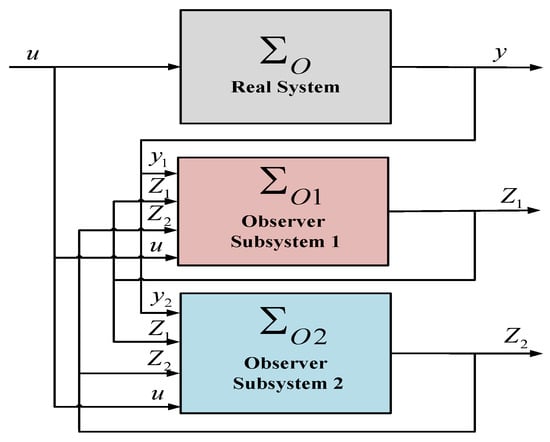
Figure 1.
Proposed cascade nonlinear observer block diagram.
3.3. Analysis of Cascade Nonlinear Observer Stability
In this subsection, we present the stability analysis of the designed cascade nonlinear observer. We define the estimate errors and as , . The first derivatives of and are given by
We make the definitions and . The first derivatives of and are
where and are
Assumption 2.
In this paper, the notation denotes the Euclidean norm (L2 norm) for vectors, defined as for the vector . For matrices, is defined as for the matrix . This assumption is verified because of the bounds of the considered state variables (Assumption 2) and the persistent. The norm notation used throughout this paper denotes the Euclidean norm for vectors and the Frobenius norm for matrices, unless otherwise specified.
Lemma 1.
Proof.
Consider the candidate Lyapunov function V as follows:
where and , and ; ; and .
We calculate the first time derivative of V and we obtain
With Assumptions 1 and 2 we get
Then
where and are positive constants that are chosen to satisfy the Lipschitz conditions, the inequalities in (37), and the following equation:
We rewrite the terms of the Lyapunov functions and as follows:
The above inequalities can be expressed with the following compact form:
with
Finally, with , we obtain
where is such that .
Taking , and letting , we then have
That is the end of the proof. □
4. Adaptive Twisting Controller Design
In the LIM system, the mathematical relationship between and and and can be expressed as
where is the induced-part flux angle, and is the induced-part flux vector rotational speed.
By using the indirect field-oriented control (IRFOC) strategy [30] in the LIM system (), the state-space Equations (1)–(5) of the LIM can be expressed in the inductor-part flux reference frame ( axis) as follows:
The control objective is to force the LIM speed v and rotor flux to track the desired LIM speed and rotor flux . By using IRFOC theory, twisting sliding mode controllers with an adaptation algorithm [21] are successfully applied to the LIM system. Here, we define two tracking errors, and , as
where , are the desired rotor flux and desired LIM speed, respectively; and ; is the estimated speed error; and is the estimated flux error, where and can be calculated:
From the stability analysis of the cascade nonlinear observer designed above, ; ; and . Obviously, we obtain and .
The first derivatives of and are
The second derivatives of and are
We define two new variables, and , as and ; we have
where the disturbances and are
where and are two bounded disturbances with the unknown boundaries , and , , which satisfy
The ATCs and are designed as follows:
where the adaptive gains and are obtained through [21]
with
where
By choosing appropriate parameters for the adaptation algorithm, the ATCs can achieve finite-time convergence to the vicinity of zero, despite the presence of two bounded disturbances, and , with unknown boundaries [21].
5. Hardware-in-the-Loop Experiment
The proposed cascade nonlinear observer-based adaptive twisting control scheme for the LIM was tested in a hardware-in-the-loop (HIL) experiment. The overall architecture of the proposed CNO-based ATC scheme for the LIM is shown in Figure 2. It mainly consists of two DS1104 Real-Time (RT) board cards: one for the LIM controller/observer application and the other for the emulation of the LIM [31,32]. The HIL experiment test bench was implemented in real time with the sampling frequency of 10 kHz. The nominal parameters of the LIM are given in Table 1.
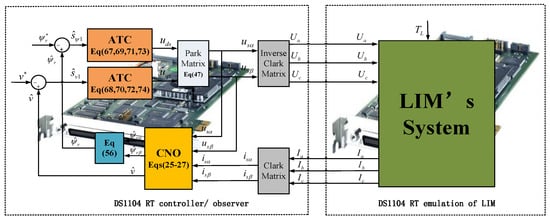
Figure 2.
Proposed CNO-ATC scheme of LIM.

Table 1.
Parameters of linear induction motor.
In the LIM system, the initial values of the state variables were set as A; A; Wb; and Wb. In the proposed cascade nonlinear observer, the designed parameters were chosen as ; ; and .
In the rotor flux adaptive twisting controller, the initial value of was set as , and the designed parameters of the adaptation algorithm were chosen as ; ; ; ; ; and , . In the LIM speed adaptive twisting controller, the initial value of was set as , and the designed parameters of the adaptation algorithm were chosen as ; ; ; ; ; ; and .
5.1. CNO Performance
To better reflect the observer performance of the designed cascade nonlinear observer, the initial values of the estimated currents and fluxes were chosen differently from those of the initial state variables, and their values were set as A; A; Wb; and Wb.
Figure 3a,b show the actual and the estimated rotor fluxes, obtained with the proposed cascade nonlinear observer, under speed square references of m/s. Correspondingly, the LIM speed estimation performance is shown in Figure 3c. In this comparative study, we conducted a systematic experimental analysis of the performance of three types of observation algorithms, namely the local cascade observation algorithm, the sliding mode observer (SMO), and the Luenberger observer. This cascade observation algorithm has higher estimation accuracy. This advantage mainly stems from its innovative multi-level signal coupling mechanism, which effectively suppresses noise interference and improves the accuracy of parameter identification.
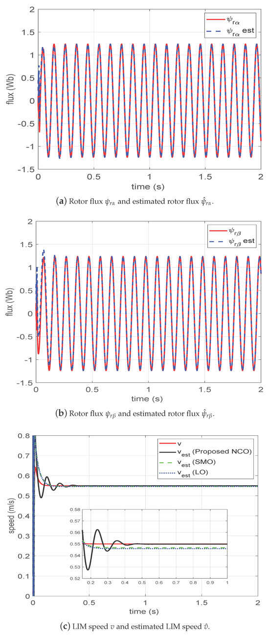
Figure 3.
Proposed CNO for LIM in nominal system with HIL experiment.
5.2. CNO-ATC Performance
In this subsection, we detail how the designed CNO-based STC scheme was implemented on a hardware-in-the-loop test bench. The reference speed signal was set as m/s, and the reference flux modulus signal was set as Wb2. The initial estimated states in the proposed cascade observer were set as A; A; Wb; and Wb.
To test the robustness property of the proposed CNO-ATC scheme, the value of the load torque was defined as follows:
5.2.1. Nominal System
Figure 4a presents the trajectories of the reference speed, the real speed, and the estimated speed in the proposed observer-based controller scheme. One can see that the estimated speed and tracking speed reached the steady state with a great dynamic response in less than 0.2 s. There existed little speed variation at s and s due to abrupt load variation, while the estimated speed accurately tracked the real speed with high estimation accuracy.
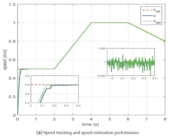
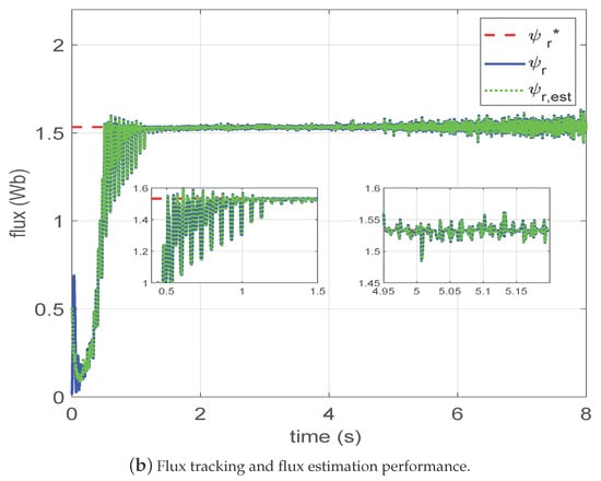
Figure 4.
Proposed CNO-ATC scheme for LIM in nominal system with HIL experiment.
Figure 4b presents the trajectories of the reference modulus flux, the real modulus flux, and the estimated modulus flux in the proposed cascade nonlinear observer-based ATC scheme. One can see that estimated modulus flux and tracking modulus flux reached the steady state with a good dynamic response in less than 0.8 s. Similarly, there existed little modulus flux variation at s and s, although the variation was very small and the estimation accuracy remained high.
5.2.2. Perturbed System
In this subsection, considering the influence of parametric uncertainties, we assume the actual to be , where .
Figure 5a presents the trajectories of the reference speed, the real speed, and the estimated speed in the proposed cascade nonlinear observer-based ATC scheme. One can see that the estimated speed and tracking speed reached the steady state with a great dynamic response in less than 0.2 s. There existed small speed variation at s and s due to abrupt load variation, while the estimated speed accurately tracked the real speed with high estimation accuracy.
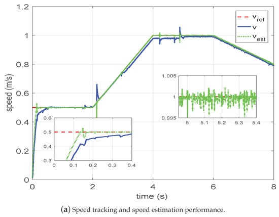
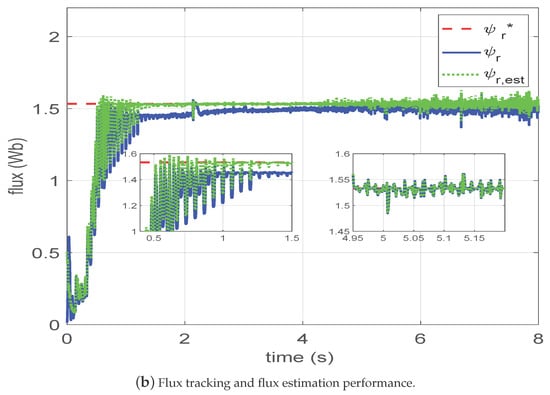
Figure 5.
Proposed CNO-ATC scheme for LIM in disturbance system with HIL experiment.
Figure 5b presents the trajectories of the reference modulus flux, the real modulus flux, and the estimated modulus flux in the proposed cascade nonlinear observer-based ATC scheme. One can see that estimated modulus flux and tracking modulus flux reached the steady state with a good dynamic response in less than 0.15 s. Similarly, there existed small modulus flux variation at s and s, although the variation was very small and the estimation accuracy was very high.
6. Conclusions
In this paper, two adaptive twisting controllers were designed for the LIM drive without mechanical sensors (speed and load torque sensors). A cascade observer was designed and applied to the linear induction motor, where the rotor fluxes and LIM speed were estimated. The proposed cascade nonlinear observer was utilized by the adaptive twisting controller in a closed loop to achieve LIM speed and flux tracking for the linear induction motor without requiring measurements of LIM speed and rotor fluxes. A detailed analysis of the convergence of the cascade nonlinear observer was presented. The CNO was tested and validated with the ATC in a closed-loop configuration using a hardware-in-the-loop experiment test bench. HIL results showed that the convergence of the designed observer was achieved, and excellent performance was obtained in the presence of variations in the rotor resistance. Moreover, the ATC-based CNO methodology can achieve accurate LIM speed and rotor flux tracking in the absence of mechanical sensors under different operating conditions.
Author Contributions
L.Z. led this research, conducted the investigation, and wrote the original draft. X.X. contributed to formal analysis and validation. D.W. and Z.W. assisted with software development and data curation. J.W., J.J., H.D., J.L., and J.H. (Jie Huang) supervised the project and provided critical revisions. J.H. (Jingli Huang), as the corresponding author, oversaw the conceptualization, funding acquisition, and overall project administration and finalized the manuscript. All authors have read and agreed to the published version of the manuscript.
Funding
This work was supported by Natural Science Foundation of China (92367109), Postdoctoral program in China (369446), Natural Science Youth Fund project of Henan Province (242300421439), Henan province key research and development and promotion of science and technology projects (232102240056), and Cultivation Programme for Young Backbone Teachers in Henan University of Technology.
Data Availability Statement
The data presented in this study are available on request from the corresponding author.
Conflicts of Interest
The authors declare no conflicts of interest.
References
- Ahmed, A.H.; Yahya, A.S.; Ali, A.J. Speed Control for Linear Induction Motor Based on Intelligent PI-Fuzzy Logic. J. Robot. Control 2024, 5, 1470–1478. [Google Scholar]
- Rametti, S.; Pierrejean, L.; Hodder, A.; Paolone, M. Pseudo-three-dimensional Analytical Model of Linear Induction Motors for high-speed applications. IEEE Trans. Transp. Electrif. 2024, 10, 9109–9120. [Google Scholar] [CrossRef]
- Shiri, A.; Tessarolo, A. Normal force elimination in single-sided linear induction motor using design parameters. IEEE Trans. Transp. Electrif. 2022, 9, 394–403. [Google Scholar] [CrossRef]
- Liu, X.; Zhao, H.; Ai, H.; Chen, Z. Design and Research on the Variable Polar Distance of the Double-Sided Linear Induction Motor for Electromagnetic Catapult. Energies 2024, 18, 33. [Google Scholar] [CrossRef]
- Wu, S.; Lu, Q. Eddy current analysis and optimization design of the secondary of the linear induction motor with an approximation and prediction method. IEEE Trans. Magn. 2021, 58, 8200105. [Google Scholar] [CrossRef]
- Xu, W.; Zou, J.; Liu, Y.; Zhu, J. Weighting factorless model predictive thrust control for linear induction machine. IEEE Trans. Power Electron. 2019, 34, 9916–9928. [Google Scholar] [CrossRef]
- Xu, W.; Ali, M.M.; Elmorshedy, M.F.; Allam, S.M.; Mu, C. One improved sliding mode DTC for linear induction machines based on linear metro. IEEE Trans. Power Electron. 2020, 36, 4560–4571. [Google Scholar] [CrossRef]
- Accetta, A.; Cirrincione, M.; Pucci, M.; Vitale, G. Closed-loop MRAS speed observer for linear induction motor drives. IEEE Trans. Ind. Appl. 2014, 51, 2279–2290. [Google Scholar] [CrossRef]
- Duncan, J. Linear induction motor-equivalent-circuit model. IEE Proc.-Electr. Power Appl. 1983, 130, 51–57. [Google Scholar] [CrossRef]
- Pucci, M. State space-vector model of linear induction motors. IEEE Trans. Ind. Appl. 2013, 50, 195–207. [Google Scholar] [CrossRef]
- Zhang, L.; Obeid, H.; Laghrouche, S.; Cirrincione, M. Second order sliding mode observer of linear induction motor. IET Electr. Power Appl. 2019, 13, 38–47. [Google Scholar] [CrossRef]
- Zhang, L.; Dong, Z.; Zhao, L.; Laghrouche, S. Sliding mode observer for speed sensorless linear induction motor drives. IEEE Access 2021, 9, 51202–51213. [Google Scholar] [CrossRef]
- Yildiz, R.; Barut, M.; Zerdali, E. A comprehensive comparison of extended and unscented Kalman filters for speed-sensorless control applications of induction motors. IEEE Trans. Ind. Inform. 2020, 16, 6423–6432. [Google Scholar] [CrossRef]
- Alonge, F.; Cirrincione, M.; D’Ippolito, F.; Pucci, M.; Sferlazza, A.; Vitale, G. Descriptor-type Kalman filter and TLS EXIN speed estimate for sensorless control of a linear induction motor. IEEE Trans. Ind. Appl. 2014, 50, 3754–3766. [Google Scholar] [CrossRef]
- Wu, L.; Liu, J.; Vazquez, S.; Mazumder, S.K. Sliding mode control in power converters and drives: A review. IEEE/CAA J. Autom. Sin. 2021, 9, 392–406. [Google Scholar] [CrossRef]
- Shi, Q.; He, S.; Wang, H.; Stojanovic, V.; Shi, K.; Lv, W. Extended state observer based fractional order sliding mode control for steer?by?wire systems. IET Control Theory Appl. 2024, 18, 2287–2295. [Google Scholar] [CrossRef]
- Mousavi, Y.; Bevan, G.; Kucukdemiral, I.B.; Fekih, A. Sliding mode control of wind energy conversion systems: Trends and applications. Renew. Sustain. Energy Rev. 2022, 167, 112734. [Google Scholar] [CrossRef]
- Zhang, J.; Zhu, D.; Jian, W.; Hu, W.; Peng, G.; Chen, Y.; Wang, Z. Fractional order complementary non-singular terminal sliding mode control of PMSM based on neural network. Int. J. Automot. Technol. 2024, 25, 213–224. [Google Scholar] [CrossRef]
- Laghrouche, S.; Harmouche, M.; Chitour, Y.; Obeid, H.; Fridman, L.M. Barrier function-based adaptive higher order sliding mode controllers. Automatica 2021, 123, 109355. [Google Scholar] [CrossRef]
- Ye, Z.; Zhang, D.; Cheng, J.; Wu, Z. Event-triggering and quantized sliding mode control of UMV systems under DoS attack. IEEE Trans. Veh. Technol. 2022, 71, 8199–8211. [Google Scholar] [CrossRef]
- Shtessel, Y.B.; Moreno, J.A.; Fridman, L.M. Twisting sliding mode control with adaptation: Lyapunov design, methodology and application. Automatica 2017, 75, 229–235. [Google Scholar] [CrossRef]
- Razmjooei, H.; Palli, G.; Abdi, E.; Terzo, M.; Strano, S. Design and experimental validation of an adaptive fast-finite-time observer on uncertain electro-hydraulic systems. Control Eng. Pract. 2023, 131, 105391. [Google Scholar] [CrossRef]
- Yan, Z.; Deng, S.; Yang, Z.; Zhao, X.; Yang, N.; Lu, Y. Improved nonlinear active disturbance rejection control for a continuous-wave pulse generator with cascaded extended state observer. Control Eng. Pract. 2024, 146, 105897. [Google Scholar] [CrossRef]
- Farza, M.; Hernández-González, O.; Ménard, T.; Targui, B.; M’Saad, M.; Astorga-Zaragoza, C. Cascade observer design for a class of uncertain nonlinear systems with delayed outputs. Automatica 2018, 89, 125–134. [Google Scholar] [CrossRef]
- Holakooie, M.H.; Ojaghi, M.; Taheri, A. Full-order Luenberger observer based on fuzzy-logic control for sensorless field-oriented control of a single-sided linear induction motor. Isa Trans. 2016, 60, 96–108. [Google Scholar] [CrossRef]
- Wang, Z.; Sun, W.; Jiang, D.; Qu, R. Observability Analysis of Q-MRAS Drive of Induction Motor With and Without Virtual Voltage Injection. In Proceedings of the 2019 22nd International Conference on Electrical Machines and Systems (ICEMS), Harbin, China, 11–14 August 2019; pp. 1–6. [Google Scholar]
- Paradowski, T.; Tibken, B.; Swiatlak, R. An approach to determine observability of nonlinear systems using interval analysis. In Proceedings of the 2017 American Control Conference (ACC), Seattle, WA, USA, 24–26 May 2017; pp. 3932–3937. [Google Scholar]
- Martinelli, A. Nonlinear unknown input observability: Extension of the observability rank condition. IEEE Trans. Autom. Control 2018, 64, 222–237. [Google Scholar] [CrossRef]
- Ran, M.; Li, J.; Xie, L. A new extended state observer for uncertain nonlinear systems. Automatica 2021, 131, 109772. [Google Scholar] [CrossRef]
- Zhang, L.; Obeid, H.; Laghrouche, S. Adaptive twisting controller for linear induction motor considering dynamic end effects. In Proceedings of the 2018 15th International Workshop on Variable Structure Systems (VSS), Graz, Austria, 9–11 July 2018. [Google Scholar]
- Gong, W.; Liu, C.; Zhao, X.; Xu, S. A model review for controller-hardware-in-the-loop simulation in EV powertrain application. IEEE Trans. Transp. Electrif. 2023, 10, 925–937. [Google Scholar] [CrossRef]
- Dai, X.; Ke, C.; Quan, Q.; Cai, K.-Y. RFlySim: Automatic test platform for UAV autopilot systems with FPGA-based hardware-in-the-loop simulations. Aerosp. Sci. Technol. 2021, 114, 106727. [Google Scholar] [CrossRef]
Disclaimer/Publisher’s Note: The statements, opinions and data contained in all publications are solely those of the individual author(s) and contributor(s) and not of MDPI and/or the editor(s). MDPI and/or the editor(s) disclaim responsibility for any injury to people or property resulting from any ideas, methods, instructions or products referred to in the content. |
© 2025 by the authors. Licensee MDPI, Basel, Switzerland. This article is an open access article distributed under the terms and conditions of the Creative Commons Attribution (CC BY) license (https://creativecommons.org/licenses/by/4.0/).