Coordinated Control for Stability of Four-Wheel Steering Vehicles Based on Game Theory

Abstract

To address the poor stability of four-wheel steering vehicles under extreme conditions, this paper proposes a coordinated control strategy for vehicles with four-wheel independent drive. The strategy combines the Active Four-Wheel Steering system with the Direct Yaw Moment Control system. First, a shared steering control model is constructed by considering both the vehicle’s path-tracking performance and handling stability. Based on this model, a control strategy for the four-wheel steering system is proposed using a non-cooperative Nash game. Next, a direct yaw moment controller is designed to improve vehicle lateral stability under dangerous driving conditions. To achieve synergy between rear-wheel steering and direct yaw moment control, a rule-based coordination strategy is introduced to optimize the working intervals of each sub-controller. Finally, experimental verification is performed under double-lane-change and slalom conditions using the CarSim/Simulink hardware-in-the-loop platform. All computations were done in MATLAB R2024a, using specific m-files and Simulink functions for implementation, and the controller was implemented using the Micro-Autobox tool. The results demonstrate that the proposed control strategy significantly enhances vehicle path-tracking accuracy and handling stability under extreme driving conditions.

1. Introduction

With the growing prominence of energy crises and traffic safety issues, electrification and intelligentization have become the core development directions of the automotive industry [1]. Among them, four-wheel steering/four-wheel independent drive vehicles have emerged as a research focus in the field of automotive engineering due to their advantages such as fast response speed, high control precision, and ease of implementing active chassis control.

At present, the technology of intelligent electric vehicles is advancing continuously, with their driving speed increasing and operating environment becoming increasingly complex [2]. As a typical highly nonlinear system, a vehicle, when driving at high speeds, is not only subject to its own dynamic constraints but also affected by external factors such as road adhesion conditions, crosswinds, and road curvature. In particular, when driving on roads with low adhesion coefficients and large curvatures, it is highly prone to instability. Therefore, ensuring the stability of path tracking for intelligent electric vehicles under extreme working conditions is of great research value.

Based on the steering control methods, vehicles can be categorized into Active Front Steering (AFS), Active Rear Steering (ARS), and Four-Wheel Steering (4WS) systems. Currently, the AFS system is the most commonly used steering control method. Although the AFS system provides excellent maneuverability at low speeds, as the vehicle speed increases, the lateral force on the front tires is prone to reach saturation, making it difficult to generate sufficient lateral force to maintain vehicle stability. In contrast, the 4WS system allows for the steering of the front and rear wheels in opposite directions at low speeds, resulting in a smaller turning radius and improved vehicle handling. At high speeds, the 4WS system coordinates the steering of the front and rear wheels in the same direction, enhancing vehicle stability, reducing body roll, and preventing skidding, thereby improving driving safety [3,4,5,6].

Currently, research on stability coordinated control for four-wheel steering/four-wheel drive vehicles mainly focuses on two directions: active rear-wheel steering and active four-wheel steering. Ref. [7] proposes an active rear-wheel steering control system composed of a radial basis function neural network controller and a single-neuron adaptive PSD (Proportional Sum Differential) controller; Ref. [8] designs a variable weight coefficient LQR (Linear Quadratic Regulator) active rear-wheel steering control strategy based on road adhesion coefficients; Ref. [9] constructs a non-sliding finite-time convergence controller for active four-wheel steering control of vehicles by improving the sliding mode control algorithm; Ref. [10] designs an active four-wheel steering control system with double-layer dynamic decoupling control based on diagonal decoupling methods and model predictive control theory; Ref. [11] puts forward a three-step active four-wheel steering controller consisting of quasi-steady-state control, feedforward control, and feedback control. Although the above studies have effectively improved the handling stability of vehicles during path tracking by combining the performance advantages of various systems, they all coordinate multiple control systems through integrated or hierarchical control strategies and fail to fully consider the reverse impact of stability control on the path-tracking system, that is, excessive additional yaw moments or rear-wheel angles may reduce path-tracking accuracy to a certain extent. Dynamic game theory, however, provides an effective approach to solving interaction problems between multiple agents [12,13].

Four-wheel steering vehicles can improve stability by controlling wheel angles to change tire lateral forces. Nevertheless, under extreme working conditions, when the tire lateral force reaches saturation, the four-wheel steering controller will lose its ability to regulate vehicle stability. Therefore, it is necessary to introduce tire longitudinal force control to enhance the stability of four-wheel steering vehicles under extreme working conditions. At present, research on Direct Yaw Moment Control (DYC) has been relatively mature, mostly adopting a hierarchical control architecture: the upper layer calculates the additional yaw moment, and the lower layer completes the optimal torque distribution through quadratic programming algorithms [14,15]. To improve vehicle response speed, most upper-layer controllers are designed based on linear tire models [16]; however, vehicle instability mostly occurs in the nonlinear region of tires, and such models have problems such as low control precision and poor control effect. Some scholars have proposed nonlinear MPC control strategies [17,18] and described the nonlinear characteristics of tires based on the magic formula, but this increases the complexity of the model [19,20,21]. Therefore, designing a simple and efficient DYC controller is of great significance for improving the lateral stability of vehicles.

Both the Active Rear-wheel Steering (ARS) system and the DYC system aim to improve the lateral stability of vehicles, and the coordinated control between them is a current research difficulty. Ref. [22] designs an adaptive optimal controller based on Lagrangian neural networks for the coordinated control of four-wheel steering and direct yaw moment, with the direct yaw moment distribution adopting a four-wheel drive/braking force coordinated distribution method; Ref. [23] designs a coordinated controller of active rear-wheel steering and direct yaw moment based on sliding mode control theory, with the direct yaw moment distribution using a four-wheel braking force distribution method; Ref. [24] designs an integrated control algorithm of four-wheel steering and direct yaw moment through sliding mode control, and simultaneously develops an electronic booster with both brake booster and wheel cylinder pressure regulation functions for the integrated control system, with the direct yaw moment distribution selecting a rule-based single-wheel braking method; Ref. [25] combines fuzzy control and sliding mode control theory to design a coordinated control system of active rear-wheel steering and direct yaw moment, with the direct yaw moment distribution adopting a two-front-wheel ABS (Anti-lock Brake System) braking force distribution method. Although the above studies have achieved good results in improving vehicle stability under extreme working conditions, they have ignored the problem of insufficient steering sensitivity of four-wheel steering vehicles under high-speed stable driving conditions, which will reduce the high-speed emergency obstacle avoidance capability of vehicles. Therefore, it is necessary to design a direct yaw moment controller to improve the steering sensitivity of four-wheel steering vehicles under high-speed stable driving conditions by adjusting their yaw rate response.

In existing studies, research on Active Front-wheel Steering (AFS), ARS, and DYC mainly focuses on uncoordinated control systems. The stability system only responds to the upper path-tracking system (AFS) and does not consider its impact on path-tracking performance. In fact, the yaw moment or rear-wheel angle determined by the stability system will change the vehicle driving path, and the AFS system will update the front-wheel angle control command to track the target path. Therefore, it is necessary to establish a coordinated controller between the path-tracking and stability systems to reflect the information interaction and transmission between agents. Based on this, the main research contents of this paper are as follows:

(1)

For the AFS and ARS systems, construct a new shared steering control model and propose an active 4WS control strategy based on the Nash game.

(2)

Design a DYC system based on sliding mode control to improve the maneuverability and stability of the vehicle under extreme working conditions.

(3)

Establish a rule-based ARS/DYC coordinated controller to realize the coordinated control of stability systems under dangerous driving conditions of the vehicle.

To emphasize the novelty and contributions of our work, we have included a comparison table (Table 1) that highlights the key differences between our research and other related works. This table summarizes the control strategies, methodologies, and innovations from the literature, as well as the limitations that each approach faces. By comparing these works, we demonstrate how our proposed coordinated control strategy based on the Active Four-Wheel Steering system and Direct Yaw Moment Control system offers distinct advantages in terms of vehicle stability and path-tracking accuracy under extreme driving conditions, as shown in Table 1.

Table 1. Comparison table.

Reference	Control Strategy	Key Methodology	Key Contributions/Innovations
Wang et al. (2020) [1]	Coordinated control of four-wheel steering	Nash game-based strategy for four-wheel steering and direct yaw moment control	Integration of 4WS and DYC for improved stability and handling accuracy
Li et al. (2016) [7]	Vehicle stability control	Integration of DYC with active rear steering	Focus on lateral stability enhancement in extreme conditions
Gao et al. (2017) [24]	Integrated stability control	Nash game for coordination of 4WS and DYC	Improved vehicle stability and maneuverability during extreme conditions
Demirci & Gokasan (2013) [22]	Adaptive control for 4WS-4WD vehicles	Lagrangian neural networks for stability control of 4WS	Adaptive optimal control strategy for improved stability
This Study	Coordinated control of 4WS and DYC	Nash game-based coordination, fuzzy neural network for ARS/DYC coordination	Effective path-tracking and stability control under extreme driving conditions

The remaining structure of the paper is as follows: Section 2 introduces the system model; Section 3 proposes the Coordinated Control for Stability of Four-Wheel Steering vehicles; Section 4 shows the simulation and experimental results and analysis; Section 5 summarizes the research conclusions.

2. Vehicle Dynamics Model

In this section, we present the vehicle dynamics model that underpins the development of the proposed control strategy. The model focuses on the essential aspects of vehicle motion, including lateral dynamics and yaw motion, which are critical for ensuring stability and accurate path tracking. To simplify the model and enhance computational efficiency, several assumptions are made, which form the foundation of the control strategy and help to address the complexities inherent in real-world driving conditions. The following subsection outlines these assumptions and their impact on the control system design.

2.1. Assumptions

To simplify the model derivation, enhance computational efficiency, and ensure the practicality of the study, several assumptions are made in this paper. These assumptions form the foundation of the control strategy and vehicle dynamics model. The specific assumptions are as follows:

Assumption 1. 

The road surface adhesion coefficient is assumed to be constant.

In the control system design, it is assumed that the road surface adhesion coefficient does not vary over time, which helps simplify the model. However, in reality, the adhesion coefficient can fluctuate.

Impact: This assumption simplifies the modeling of road condition changes, ensuring that the control algorithm performs effectively under stable adhesion conditions. However, in real-world applications, variations in the road adhesion coefficient may require adaptive control strategies to handle such changes.

Assumption 2. 

Wind effects on vehicle motion are neglected.

For simplicity, it is assumed that the vehicle is not influenced by external factors such as crosswinds during operation. However, in complex environments, wind conditions could affect vehicle stability.

Impact: Neglecting wind effects makes the analysis simpler, but under adverse weather conditions, wind could significantly impact vehicle stability. Future studies can consider incorporating wind effects into the model.

Assumption 3. 

The tire model is assumed to be linear.

The lateral and longitudinal forces of the tire are assumed to be linearly related, though in reality, the tire’s behavior may be nonlinear under high slip angles.

Impact: The linear tire model simplifies the system’s computation, but it may have limitations in high-slip scenarios where the tire’s nonlinearity becomes more pronounced. Future work could explore more complex nonlinear tire models.

Assumptions 4. 

The vehicle dynamic model is a 2-degree-of-freedom (2DOF) model. This model is applicable when the vehicle is in uniform circular motion, and in this state, the parameter values of the vehicle in a stable state can be obtained.

Impacts: The 2DOF model provides convenience for simplified analysis.

2.2. WS Dynamics Model

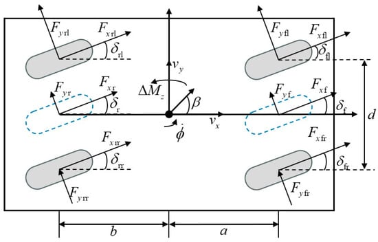
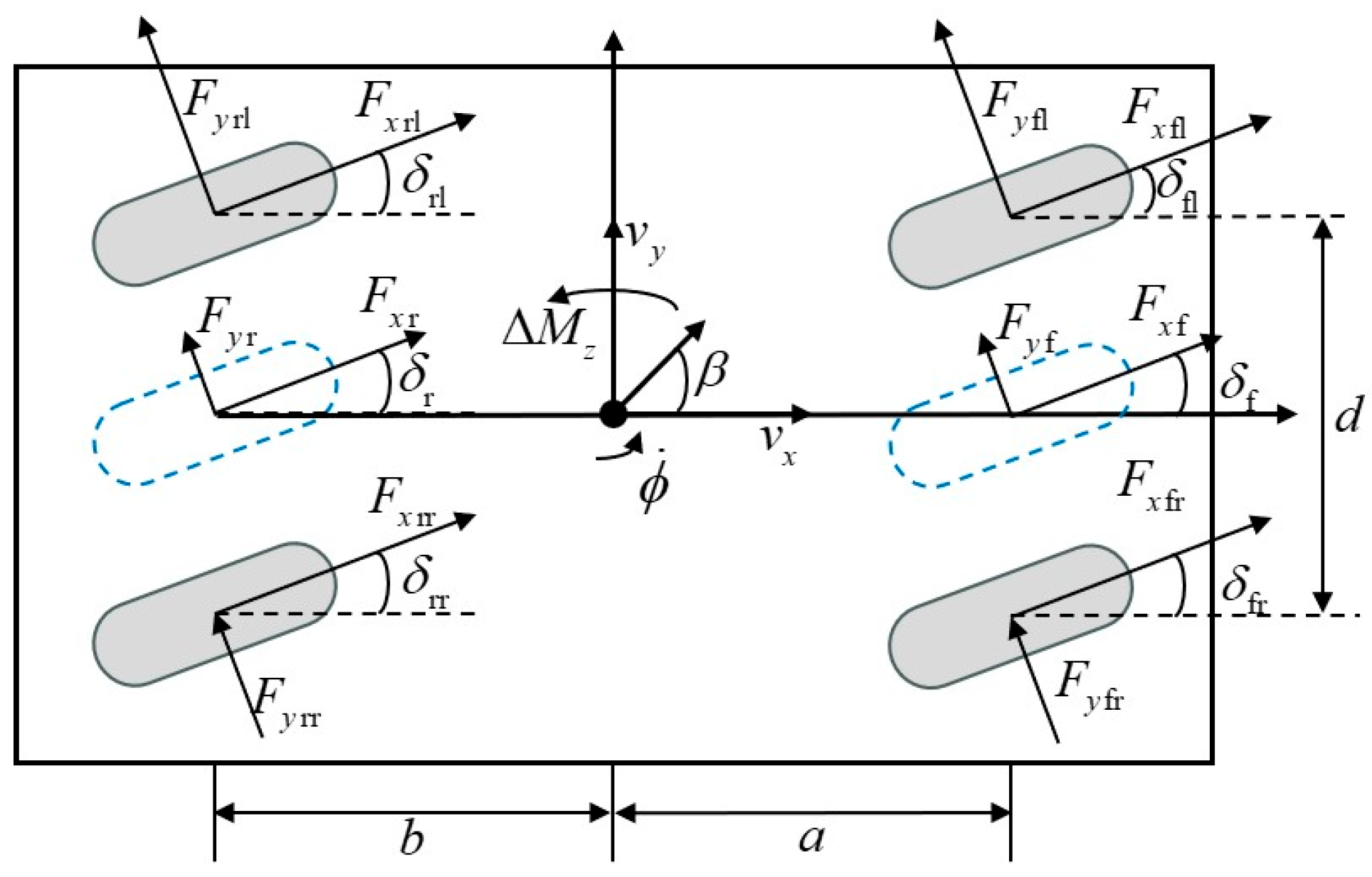
During the vehicle driving process, the linear 2-degree-of-freedom (2DOF) vehicle dynamics model can relatively accurately reflect the vehicle steering response characteristics under small steering angle conditions and within the linear working region of the tires. Based on this, this section limits the research focus to the influence of the vehicle lateral motion and yaw motion on driving stability, and the established 4WS vehicle dynamics model is shown in Figure 1.

Figure 1. Diagram of the 4WS Vehicle Model.

The state equation of linear two-degree-of-freedom (2DOF) vehicle dynamics is as follows:

$$\dot{X}=AX+BU+EW$$

(1)

In the Formula (1), $X=\left[\begin{array}{l}\beta \\ \dot{\varphi }\end{array}\right]$; $U=\left[\begin{array}{l}{\delta }_f\\ {\delta }_r\end{array}\right]$; $W=\left[\Delta M_z\right]$; $A=\left[\begin{array}{cc}{a}_{11}& a_{12}\\ a_{21}& a_{22}\end{array}\right]$; $B=\left[\begin{array}{cc}{b}_{11}& b_{12}\\ b_{21}& b_{22}\end{array}\right]$; $E=\left[\begin{array}{c}0\\ 1/I_z\end{array}\right]$.

The parameter definitions of the dynamic model are as follows:

$$\left\{\begin{array}{l}{a}_{11}=-{\displaystyle \frac{k_1+k_2}{m{v}_x}}\\ a_{12}={\displaystyle \frac{b{k}_2-a{k}_1}{m{v}_x^2}}-1\\ a_{21}={\displaystyle \frac{b{k}_2-a{k}_1}{I_z}}\\ a_{22}=-(a^2{k}_1+b^2{k}_2)/I_z{v}_x\end{array}\right.$$

(2)

$$\left\{\begin{array}{l}{b}_{11}=k_1/m{v}_x\\ b_{12}=k_2/m{v}_x\\ b_{21}=a{k}_1/I_z\\ b_{22}=-b{k}_2/I_z\end{array}\right.$$

(3)

In the Formula (3), m is the vehicle mass; $\beta$ and $\dot{\varphi }$ are the sideslip angle at the center of mass and the yaw rate, respectively; $I_z$ is the moment of inertia of the vehicle around the z-axis; $a$ and $b$ are the distances from the vehicle center of mass to the front axle and rear axle, respectively; ${\delta }_f$ and ${\delta }_r$ are the front wheel steering angle and rear wheel steering angle, respectively; $\Delta M_z$ is the additional yaw moment.

2.3. Path-Tracking Model

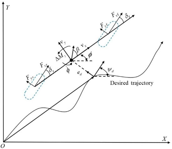
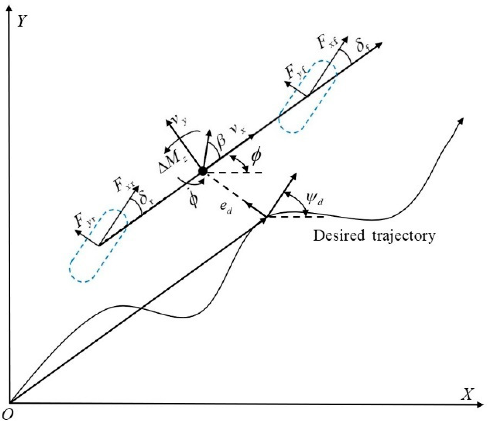
In this section, we present the path-tracking model used to describe the vehicle motion during trajectory tracking. The model is based on the displacement error $e_d$ and heading error $e_{\psi }$, which are essential for assessing the vehicle tracking performance. The following Figure 2 illustrates the path-tracking model used in this study.

Figure 2. Diagram of the Path-Tracking Model.

As shown in Figure 2, in the path-tracking system, the displacement error $e_d$ and heading error $e_{\psi }$ are primarily used to measure the vehicle path-tracking accuracy. $e_d$ represents the displacement deviation of the vehicle center of mass from the road centerline, and $e_{\psi }$ denotes the deviation between the vehicle yaw angle $\varphi$ at the center of mass and the road’s reference heading angle ${\psi }_d$. The path-tracking model is expressed as follows:

$$\left\{\begin{array}{l}{\dot{e}}_d=v_y+v_x{e}_{\psi }=v_x\beta +v_x{e}_{\psi }\\ {\dot{e}}_{\psi }=\dot{\varphi }-{\dot{\psi }}_d=\dot{\varphi }-k_r\dot{s}\end{array}\right.$$

(4)

In the Formula (4), $k_r$ is the curvature of the reference path; $s$ is the velocity projection of the vehicle center of mass in the natural coordinate system.

Equation (1) can be transformed into the following form:

$$\dot{z}=Az+F_1{\delta }_f+F_2{\delta }_r$$

(5)

In Formula (5), $F_1={\left[b_{11},b_{21}\right]}^T$; $F_2={\left[b_{12},b_{22}\right]}^T$; and $z=X$.

By combining the vehicle dynamics model Equation (5) and the path-tracking model Equation (4), a new state equation is constructed as follows:

$${\dot{z}}^{\ast }=E^{\ast }{z}^{\ast }+F_1^{\ast }{\delta }_f+F_2^{\ast }{\delta }_r+D^{\ast }{\dot{\psi }}_d$$

(6)

In Formula (6),

$$\left\{\begin{array}{l}{z}^{\ast }=\left[\begin{array}{l}{e}_d\\ e_{\psi }\\ \beta \\ \dot{\varphi }\end{array}\right];F_1^{\ast }=\left[\begin{array}{l}0\\ 0\\ b_{11}\\ b_{21}\end{array}\right];F_2^{\ast }=\left[\begin{array}{l}0\\ 0\\ b_{12}\\ b_{22}\end{array}\right]\\ E^{*}=\left[\begin{array}{cccc}0& v_x& v_x& 0\\ 0& 0& 0& 1\\ 0& 0& a_{11}& a_{12}\\ 0& 0& a_{21}& a_{22}\end{array}\right];D^{*}=\left[\begin{array}{l}0\\ -1\\ 0\\ 0\end{array}\right]\end{array}\right.$$

(7)

Due to the inherent nonlinear characteristics of automobiles, there exists a deviation between the actual driving state of the vehicle and the ideal state parameters. The rear wheel steering angle of the vehicle is controlled to track the target state parameters.

$${\dot{e}}_z=A{e}_e+F_2{\delta }_r$$

(8)

In Formula (8),

$$\left\{\begin{array}{l}{e}_z={\left[\begin{array}{cc}\beta -{\beta }_{ref}& \dot{\varphi }-{\dot{\varphi }}_{rref}\end{array}\right]}^T={\left[\begin{array}{cc}\Delta \beta & \Delta w\end{array}\right]}^T\\ w_{rref}=\min \left\{{\displaystyle \frac{v_x{\delta }_f}{(1+K{v}_v^2)l}},{\displaystyle \frac{0.85\mu g}{v_x}}\right\}\\ {\beta }_{ref}=\min \left\{{\displaystyle \frac{b+ma{v}_x/(k_{2}l)}{(1+K{v}_v^2)l}}{\delta }_f,({\displaystyle \frac{b}{v_v^2}}+{\displaystyle \frac{ma}{k_{2}l}})\mu g\right\}\end{array}\right.$$

(9)

By combining Equations (4) and (5), the shared steering model of the AFS/ARS system is obtained, which comprehensively reflects the path-tracking and handling stability performance of the vehicle:

$$\dot{x}=A_{d}x+B_1{\delta }_f+B_2{\delta }_r+Y{\dot{\psi }}_d$$

(10)

where $B_1=\left[\begin{array}{ccc}{F}_1^{*}& 0& 0\end{array}\right]$, $B_2=\left[\begin{array}{cc}{F}_2^{*}& F_2\end{array}\right]$, $Y={\left[\begin{array}{ccc}{D}^{*}& 0& 0\end{array}\right]}^T$, $x={\left[\begin{array}{cc}{z}^{*}& e_z\end{array}\right]}^T$, $A_d=\mathrm{diag}(E^{*},A)$.

3. Control System Design

In this section, the design of the control system for the vehicle is presented, with a focus on the integration of the 4WS control and stability management. The key components and methodologies used in the design, which are crucial for enhancing vehicle stability and performance, will be discussed.

3.1. Control System Structure

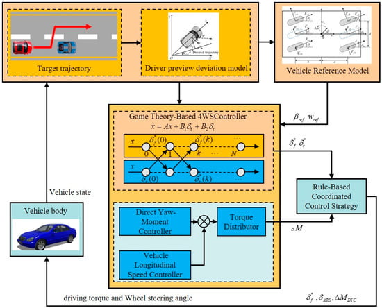
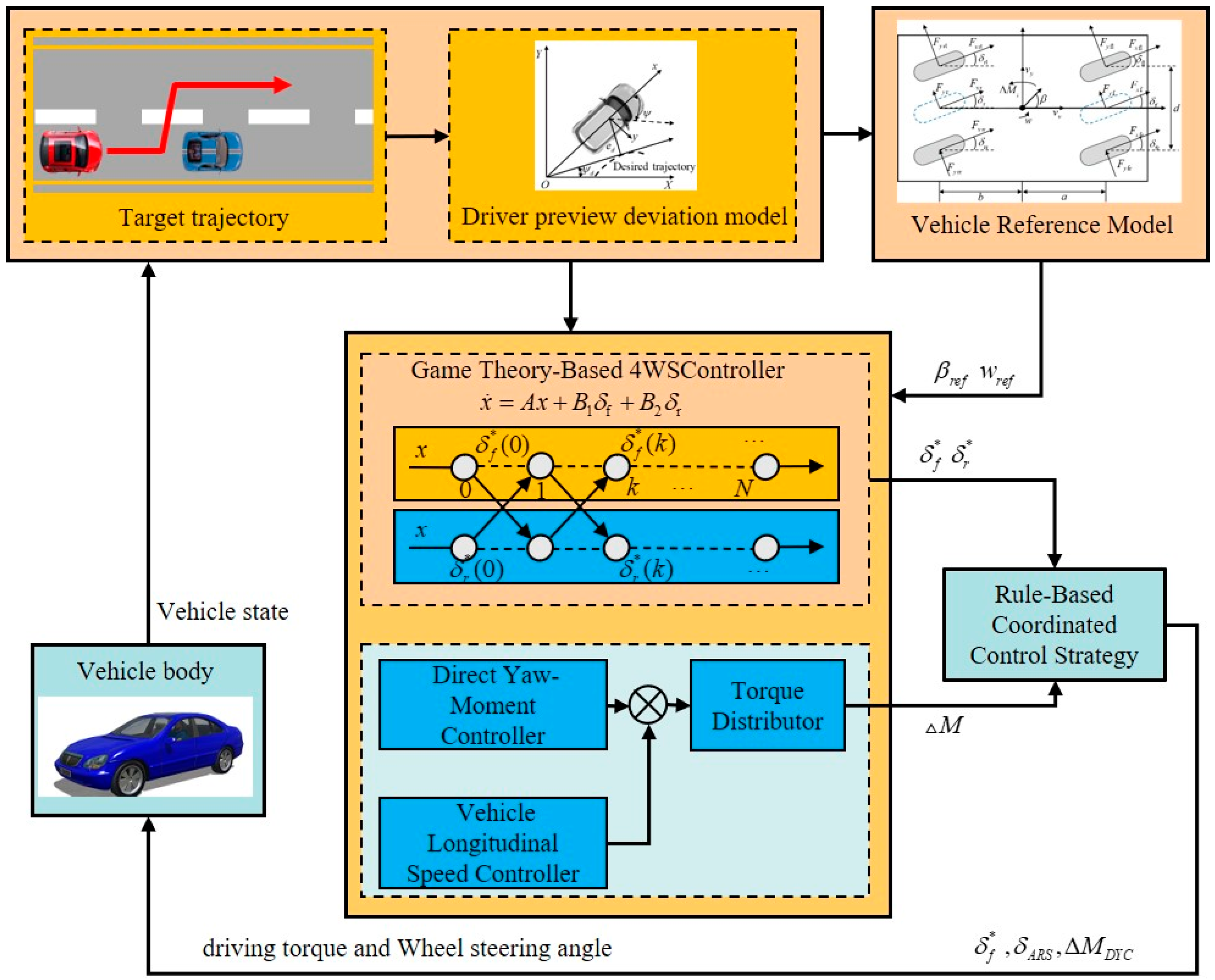
The architecture of the control system, as shown in Figure 3, mainly consists of three parts: the signal input layer, the control decision—making layer, and the control execution layer.

Figure 3. Architecture Diagram of the Control System.

The signal input layer is responsible for processing the input signals of the control system, and its input information mainly includes the driver’s input and the desired state quantities calculated by the vehicle reference model.

The control decision—making layer contains three core controllers: a 4WS controller based on Nash game, a DYC controller, and a rule—based ARS/DYC coordination controller. Among them, the 4WS controller dynamically determines the front and rear wheel angles ${\delta }_r^{*}$ and ${\delta }_f^{*}$ of the vehicle through the Nash game, realizing the sharing of steering control between the AFS and ARS systems; the DYC controller works in coordination with the 4WS controller to improve the driving stability of the vehicle. The ${\delta }_r^{*}$ determined by the 4WS controller and the $\Delta M$ control command generated by the DYC controller are jointly transmitted to the coordination controller, which calculates the weighted control quantities ${\delta }_{ARS}$ and $\Delta M_{DYC}$. The control quantities calculated by the control strategy layer will be transmitted to the control execution layer.

The control execution layer takes the vehicle model as the carrier, receives the control signals output by the control allocation layer, and feeds back the actual state information of the vehicle in real time, thus forming a hierarchical and coordinated closed-loop control process.

3.2. WS Control Based on Game Theory

Game theory can be divided into cooperative games and non-cooperative games according to the differences in the control objectives of the game subjects. Cooperative games aim to maximize collective interests. In contrast, non-cooperative games focus solely on maximizing individual interests. This distinction plays a crucial role in the coordination of steering control strategies. The AFS system is mainly used for path-tracking control, which improves the path-tracking accuracy by calculating the optimal front wheel steering angle ${\delta }_f$. The ARS system is mainly used for stability control, which improves the vehicle handling stability by deciding the optimal rear wheel steering angle ${\delta }_r$. At the same time, the ARS can compensate for vehicle instability caused by incorrect steering operations of the AFS, and the AFS can better maintain the vehicle attitude by estimating the impact of the ARS angle on vehicle state parameters. There is a relationship of information interaction and transmission between the two systems. Therefore, this section establishes a 4WS control strategy based on non-cooperative Nash game.

The AFS is defined as Game Object 1, and the ARS is defined as Game Object 2, respectively. The quadratic cost functions of both game parties are defined to represent the objective functions of the game control.

$$\left\{\begin{array}{l}{J}_1({\delta }_f,{\delta }_r)={\displaystyle \frac{1}{2}}{\displaystyle {\int }_0^{\infty }\left\{x^T(t)Q_{1}x(t)+{\delta }_f^T(t)R_{11}{\delta }_f(t)+{\delta }_r^T(t)R_{12}{\delta }_r(t)\right\}dt}\\ J_2({\delta }_f,{\delta }_r)={\displaystyle \frac{1}{2}}{\displaystyle {\int }_0^{\infty }\left\{x^T(t)Q_{2}x(t)+{\delta }_f^T(t)R_{21}{\delta }_f(t)+{\delta }_r^T(t)R_{22}{\delta }_r(t)\right\}dt}\end{array}\right.$$

(11)

where $Q_1=\mathrm{diag}\left[{\xi }^{e_d},{\xi }^{e_{\psi }},0,0,0.01,0.01\right]$; $Q_2=\mathrm{diag}\left[0.01,0.01,0,0,{\xi }^{\Delta \beta },{\xi }^{\Delta {\omega }_r}\right]$; $R_{11}=r_{11}$; $R_{12}=r_{12}$; $R_{21}=r_{21}$; $R_{22}=r_{22}$; $Q_i$ and $R_{ij}$ are weight matrices, respectively; ${\xi }^{e_d}$, ${\xi }^{e_{\psi }}$, ${\xi }^{\Delta \beta }$ and ${\xi }^{\Delta {\omega }_r}$ represent the weight coefficients of state variables; and $r_{ij}$ denotes the weight coefficient of control variables.

When ${\delta }_f^{*}$ and ${\delta }_r^{*}$ represent the Nash equilibrium solutions of the two game objects, respectively, their respective objective functions satisfy the following conditions:

$$\left\{\begin{array}{l}{J}_1({\delta }_f^{*},{\delta }_r^{*})\le J_1({\delta }_f,{\delta }_r^{*})\\ J_2({\delta }_f^{*},{\delta }_r^{*})\le J_1({\delta }_f^{*},{\delta }_r)\end{array}\right.$$

(12)

To calculate the Nash equilibrium state feedback control quantity, the Hamiltonian function is established based on the optimal control theory as follows:

$$\left\{\begin{array}{l}{H}_1={\displaystyle \frac{1}{2}}(x^T{Q}_{1}x+{\delta }_f^T{R}_{11}{\delta }_f+{\delta }_r^T{R}_{12}{\delta }_r)+{\lambda }_1^T(t)(A{x}_n+B_1{\delta }_f+B_2{\delta }_r)\\ H_2={\displaystyle \frac{1}{2}}(x^T{Q}_{2}x+{\delta }_f^T{R}_{21}{\delta }_f+{\delta }_r^T{R}_{22}{\delta }_r)+{\lambda }_2^T(t)(A{x}_n+B_1{\delta }_f+B_2{\delta }_r)\end{array}\right.$$

(13)

In Equation (13), the partial derivative of the control quantity is obtained by using the minimum principle as follows:

$$\left\{\begin{array}{l}{\displaystyle \frac{\partial H_1}{\partial {\delta }_f}}=R_{11}{\delta }_f+B_1^T{\lambda }_1(t)=0\\ {\displaystyle \frac{\partial H_2}{\partial {\delta }_f}}=R_{22}{\delta }_r+B_2^T{\lambda }_2(t)=0\end{array}\right.$$

(14)

The feedback Nash equilibrium solution can be obtained by sorting out as follows:

$$\left\{\begin{array}{l}{\delta }_f^{*}=-R_{11}^{-1}{B}_1^T{\lambda }_1(t)\\ {\delta }_r^{*}=-R_{22}^{-1}{B}_2^T{\lambda }_2(t)\end{array}\right.$$

(15)

According to the necessary conditions of optimal control, the equation is obtained as follows:

$$\left\{\begin{array}{l}{\dot{\lambda }}_1=-{\displaystyle \frac{\partial H_1}{\partial x}}=-Q_{1}x-A^T{\lambda }_1(t)\\ {\dot{\lambda }}_2=-{\displaystyle \frac{\partial H_2}{\partial x}}=-Q_{2}x-A^T{\lambda }_2(t)\end{array}\right.$$

(16)

Substituting Equation (14) into Equation (8) and sorting out, the following equation can be obtained:

$$\dot{x}=Ax-B_1{R}_{11}^{-1}{B}_1^T{\lambda }_1(t)-B_2{R}_{22}^{-1}{B}_2^T{\lambda }_1(t)$$

(17)

Equations (13) and (14) are combined to form the state matrix:

$$\left[\begin{array}{l}{\dot{\lambda }}_1(t)\\ {\dot{\lambda }}_2(t)\\ \dot{x}\end{array}\right]=\left[\begin{array}{ccc}-A^T& 0& -Q_1\\ -A^T& 0& -Q_2\\ -B_1{R}_{11}^{-1}{B}_1^T& -B_2{R}_{22}^{-1}{B}_2^T& A\end{array}\right]\left[\begin{array}{l}{\lambda }_1(t)\\ {\lambda }_2(t)\\ x\end{array}\right]$$

(18)

The coefficients ${\lambda }_1(t)$ and ${\lambda }_2(t)$ can be expressed by the vehicle state variable x as:

$$\left\{\begin{array}{l}{\lambda }_1(t)=K_{1}x\\ {\lambda }_1(t)=K_{2}x\end{array}\right.$$

(19)

The Nash equilibrium solution of the 4WS control system can be expressed as

$$\left\{\begin{array}{l}{\delta }_f^{*}=-R_{11}^{-1}{B}_1^T{K}_{1}x\\ {\delta }_r^{*}=-R_{22}^{-1}{B}_2^T{K}_{2}x\end{array}\right.$$

(20)

It can be known from Equation (20) that the feedback Nash equilibrium solution is actually a negative feedback coefficient independent of the initial state value of the vehicle. Therefore, when adopting the Nash equilibrium control strategy, the front and rear wheel steering control systems of the vehicle always execute the control commands calculated at the initial moment.

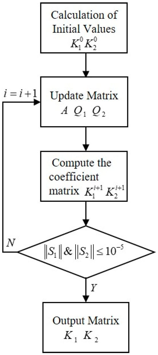
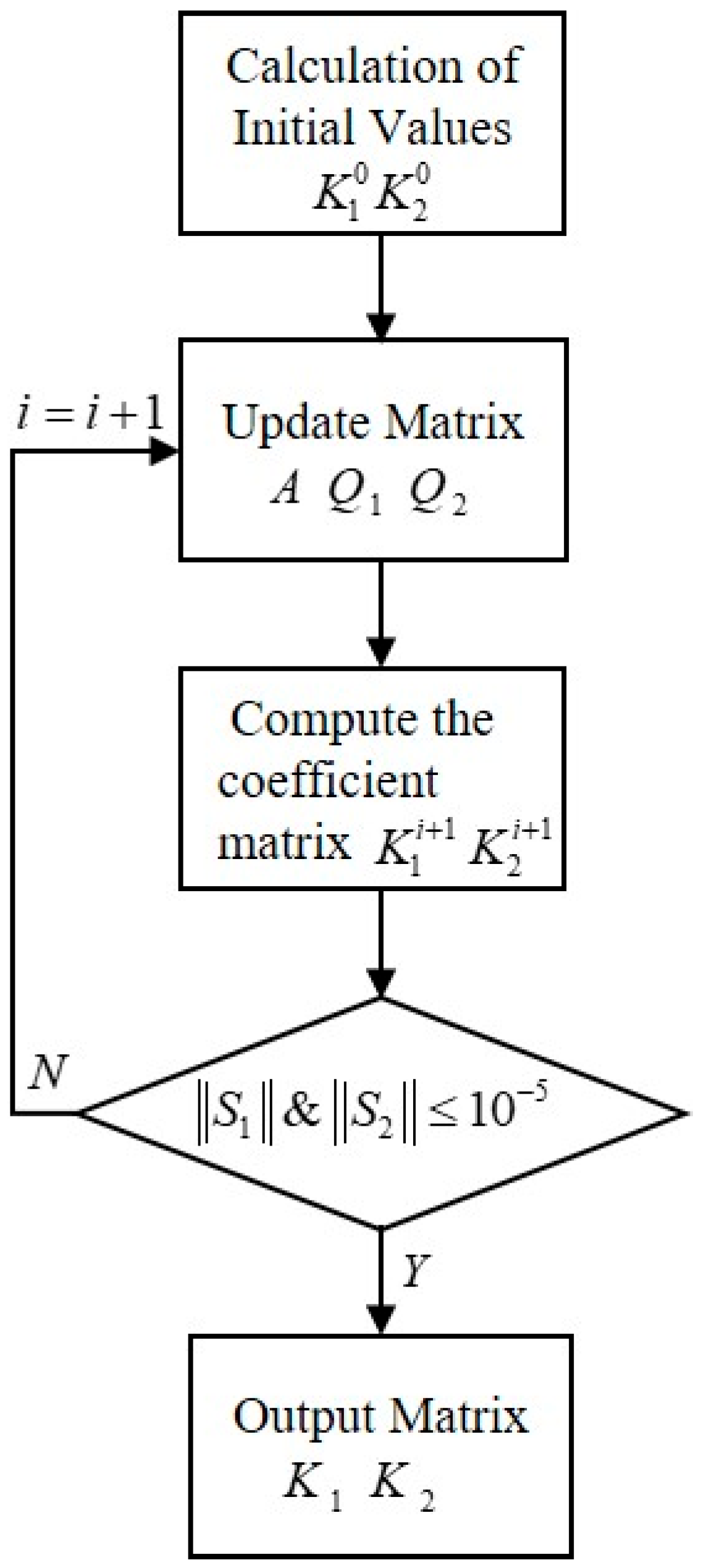
The coefficient matrices $K_1$ and $K_2$ in Equation (20) can be calculated offline through the following coupled Riccati equations:

$$\left\{\begin{array}{l}{K}_1(A-S_2{K}_2)+{(A-S_2{K}_2)}^T{K}_1+Q_1+K_2{S}_{12}{K}_2-K_1{S}_1{K}_1=0\\ K_2(A-S_1{K}_1)+{(A-S_1{K}_1)}^T{K}_2+Q_2+K_1{S}_{21}{K}_1-K_2{S}_2{K}_2=0\end{array}\right.$$

(21)

where $S_i=B_i{R}_{ii}^{-1}{B}_i^T$$S_{ij}=B_j{R}_{jj}^{-1}{R}_{ij}{R}_{jj}^{-1}{B}_j^T$.

To calculate the coupled equations, an iterative algorithm is adopted in this section to continuously update the values of the coefficient matrices $K_1$ and $K_2$, and the specific process is shown in Figure 4 [26]. Figure 4 shows the flowchart for the computation of coupled equations used to calculate the Nash equilibrium solutions in the 4WS control strategy. The process starts with calculating initial values for the coefficient matrices $K_1$ and $K_2$, followed by an iterative algorithm that continuously updates the values of these matrices until convergence is achieved. This flowchart illustrates how the iterative calculation process is applied to solve for the optimal front and rear wheel steering angles.

Figure 4. Flowchart for the computation of coupled equations.

3.3. Direct Yaw Moment Control

Under normal circumstances, during four-wheel steering, the driver’s expected driving experience should be the same as that of a front-wheel steering vehicle. That is, under the same front-wheel angle input, the same yaw rate response as that of the front-wheel steering vehicle is expected. The steady-state yaw rate of the four-wheel steering vehicle can be replaced by the steady-state yaw rate value of the front-wheel steering vehicle with the same parameters [27]. Therefore, the steady-state yaw rate of the four-wheel steering vehicle can be expressed as

$$w_{rm}=G_f{\delta }_f={\displaystyle \frac{v_x}{L(1+K{v}_x^2)}}{\delta }_f$$

(22)

where $G_f$ is the steady-state yaw rate gain from the front-wheel angle ${\delta }_f$ to the yaw rate $\dot{\varphi }$ response; $K$ is the stability coefficient, and $K=m(a/k_2-b/k_1)/L^2$.

Considering the limitation of road surface adhesion conditions and reserving a 15% road surface adhesion margin, the ideal yaw rate can be expressed as

$${\dot{\varphi }}_{rd}=min(\left|{\dot{\varphi }}_{rm}\right|,0.85\mu \mathrm{g}/v_x)\mathrm{sgn}{\delta }_f$$

(23)

where $\mu$ is the road adhesion coefficient; $g$ is the gravitational acceleration. The sliding mode surface presented in Equation (23) is selected due to its robustness against model uncertainties and external disturbances, which are inherent in vehicle dynamics, especially under extreme driving conditions. Sliding mode control (SMC) is known for its ability to handle uncertainties while ensuring fast convergence and minimizing chattering. This is particularly important in maintaining vehicle stability and achieving precise path tracking.

One of the key advantages of SMC is its robustness in handling variations in vehicle parameters. Vehicle dynamics are sensitive to changes in parameters such as tire-road friction coefficients, vehicle mass, inertia, and suspension characteristics. SMC has the capability to effectively adapt to these variations, maintaining control performance even when these parameters fluctuate. For example, changes in tire-road friction, such as in wet or icy conditions, or variations in vehicle mass or inertia, do not significantly degrade the system’s performance. The sliding mode control surface allows the system to adjust to these changes, ensuring stable and reliable vehicle performance under diverse driving conditions.

Therefore, the sliding mode surface not only provides robustness against model uncertainties but also enables the system to remain adaptive to varying vehicle parameters, making it well-suited for the coordinated control strategy, where balancing path-tracking accuracy and stability is crucial [28].

The yaw rate tracking error is defined as

$$e_{\dot{\varphi }}=\dot{\varphi }-{\dot{\varphi }}_{rref}$$

(24)

By differentiating Equation (23), considering the influence of parameter perturbation, and combining with Equation (1), it can be obtained that

$${\dot{e}}_{\dot{\varphi }}=a_{21}{v}_y+a_{22}\dot{\varphi }+b_{21}{\delta }_r+b_{22}(\Delta M_z+d(x,t))+e_{21}{\delta }_f-{\ddot{\varphi }}_{rref}$$

(25)

where $d(x,t)$ is the sum of parameter perturbations in the control system, $e_{21}={\displaystyle \frac{-a{k}_1}{I_z}}$.

Based on the yaw rate tracking error, an integral sliding mode surface is constructed, and the sliding mode surface switching function can be expressed as

$$s=e_{\dot{\varphi }}+\lambda {\displaystyle {\int }_0^t{e}_{\dot{\varphi }}dt}$$

(26)

In the Formula (26), $\lambda$ is a positive weighting coefficient, and $\lambda =7$.

When there is no parameter perturbation in the system, i.e., $d(x,t)=0$, and letting $\dot{s}=0$, the equivalent input of the additional yaw moment can be obtained as:

$$\Delta M_{z\_eq}=-{\displaystyle \frac{1}{b_{22}}}(a_{21}{v}_y+a_{22}\dot{\varphi }+b_{21}{\delta }_r+e_{21}{\delta }_f-{\ddot{\varphi }}_{rref}+\lambda e_{\dot{\varphi }})$$

(27)

When there is parameter perturbation in the system, in order to ensure that the system can still converge to the sliding mode surface, it is necessary to design a robust control law to maintain the stability of the system. The designed robust control law can be expressed as

$$\Delta M_{z\_rob}=-{\displaystyle \frac{1}{b_{22}}}(k_r\mathrm{sgn}s+k_{q}s)$$

(28)

In the Formula (28), $k_r$ and $k_q$ are the control coefficients of the exponential approaching law, with $k_r=0.1$ and $k_q=0.5$.

To verify the closed-loop stability of the control system, a Lyapunov function is defined as

$$V={\displaystyle \frac{1}{2}}{s}^2$$

(29)

Let $f(x,t)=b_{22}d(x,t)$. By differentiating Equation (28) and combining it with Equations (26) and (27), it can be obtained that

$$\dot{V}=-s{k}_r\mathrm{sgn}s-s{k}_{q}s+sf(x,t)\le -k_r\left|s\right|-k_q{s}^2+\left|s\right||f(x,t)|=-(k_r-|f(x,t)|)\left|s\right|-k_q{s}^2$$

(30)

It can be seen from Equation (30) that since both $k_r$ and $k_q$ are positive numbers, when $k_r>\left|f(x,t)\right|$, there is $\dot{V}<0$. At this point, the system is asymptotically stable in the Lyapunov sense, and the robustness of the system can be guaranteed by adjusting the parameters of the sliding mode control law.

To suppress the chattering problem occurring in the sliding mode control adjustment process, a saturation function is defined as

$$\mathrm{sat}{\displaystyle \frac{s}{\phi }}=\left\{\begin{array}{l}\mathrm{sgn}{\displaystyle \frac{s}{\phi }},|s|>\phi \\ {\displaystyle \frac{s}{\phi }},|s|\le \phi \end{array}\right.$$

(31)

In the Formula (31), $\phi$ is the boundary layer thickness, and $\phi =0.7$ [29].

Based on the above analysis, the final additional yaw moment can be obtained as

$$\Delta M_z=-{\displaystyle \frac{1}{b_{22}}}(a_{21}{v}_y+a_{22}\dot{\varphi }+b_{21}{\delta }_r+e_{21}{\delta }_f-{\ddot{\varphi }}_{rref}+\lambda e_{\dot{\varphi }}+k_r\mathrm{sat}{\displaystyle \frac{s}{\phi }}+k_{q}s)$$

(32)

3.4. Design of Longitudinal Velocity Controller

The longitudinal velocity controller is used to track the driver’s desired vehicle speed. Based on the deviation between the desired longitudinal velocity and the actual longitudinal velocity during vehicle driving, a speed-tracking PID controller is designed. The additional driving torque for tracking the desired longitudinal vehicle speed can be expressed as

$$\Delta T_v=K_P{e}_v+K_I{\displaystyle \int e_{v}dt}+K_D{\displaystyle \frac{d{e}_v}{dt}}$$

(33)

In the Formula (33), $e_v$ is the longitudinal vehicle speed deviation; $K_P$, $K_I$, and $K_D$ are the proportional coefficient, integral coefficient, and differential coefficient of the speed controller, respectively.

3.5. Design of Wheel Torque Distributor

The idea of wheel torque distribution is as follows: on the basis of the distribution of additional driving torque, the additional yaw moment is distributed, and the constraints of adhesion conditions and the external characteristics of hub motors should also be considered.

To reduce the impact of the distribution of $\Delta T_v$ on the distribution of $\Delta M_z$, $\Delta T_v$ is allocated in a four-wheel average manner. Therefore, the additional torque of each wheel for maintaining the stability of longitudinal vehicle speed can be expressed as:

$$T_{\mathrm{Basic}}={\displaystyle \frac{\Delta T_v}{4}}$$

(34)

$\Delta M_z$ is distributed through the coordinated control of driving/braking torque between the left and right wheels, and the specific torque distribution method is as follows:

$$\left\{\begin{array}{l}{T}_{a1}=-{\displaystyle \frac{F_{z1}}{F_{z1}+F_{z3}}}{\displaystyle \frac{\Delta M_{z}R}{B}}\\ T_{a2}={\displaystyle \frac{F_{z2}}{F_{z2}+F_{z4}}}{\displaystyle \frac{\Delta M_{z}R}{B}}\\ T_{a3}=-{\displaystyle \frac{F_{z3}}{F_{z1}+F_{z3}}}{\displaystyle \frac{\Delta M_{z}R}{B}}\\ T_{a4}={\displaystyle \frac{F_{z4}}{F_{z2}+F_{z4}}}{\displaystyle \frac{\Delta M_{z}R}{B}}\end{array}\right.$$

(35)

In the Formula (35), $T_{ai}$ is the additional torque of each wheel for vehicle stability control, with $i=1,2,3,4$ corresponding to the positions of the left front, right front, left rear, and right rear wheels, respectively; $F_{zi}$ is the vertical load of each wheel; $R$ is the wheel rolling radius; and $B$ is the vehicle track width.

From Equations (30) and (31), the output torque at each wheel end can be obtained as

$$T_{wi}=T_{\mathrm{Basic}}+T_{ai}$$

(36)

After being constrained by the adhesion conditions and the external characteristics of the hub motor, the final output torques at the four-wheel ends can be obtained as

$$T_{Oi}=\min (|T_{wi}|,\mu F_{zi}R,|T_{\max }|i_g)\mathrm{sgn}{T}_{wi}$$

(37)

where $T_{Oi}$ are the final output torques at the four wheel ends; $T_{\max }$ is the maximum output torque of the hub motor; $i_g$ is the reduction ratio of the hub motor reducer.

3.6. Design of Rule-Based Coordinated Control Strategy

Considering that the control target of the direct yaw moment controller is the yaw rate and it only intervenes when necessary, the yaw rate and its deviation can be used as the basis for formulating the control rules of the coordinated controller. Based on the above analysis, the control rules are formulated according to parameters such as the characteristic vehicle speed $v_{ch}$, the vehicle yaw rate $\dot{\varphi }$, the absolute value of the error of $\left|\dot{\varphi }\right|$, and four set positive control thresholds $e_1$, $e_2$, $e_4$, as shown in Table 2, where ${\dot{\varphi }}_{r\_th}=0.85\mu g/v_x$.

Table 2. Rules for coordinated control.

Judgment of Vehicle Speed	Judgment of Yaw Rate	Judgment of Yaw Rate Deviation	Control Execution Command
$v_x<v_{ch}$			ARS
$v_x\ge v_{ch}$	$\left|\dot{\varphi }\right|<\left|{\dot{\varphi }}_{r\_th}\right|$	$\left|e_{\omega }\right|\le e_1$	ARS
		$e_1<\left|e_{\omega }\right|<e_2$	ARS + DYC
		$\left|e_{\omega }\right|\ge e_2$	DYC
	$\left|\dot{\varphi }\right|\ge \left|{\dot{\varphi }}_{r\_th}\right|$	$\left|e_{\omega }\right|<e_4$	ARS + DYC
		$\left|e_{\omega }\right|\ge e_4$	DYC

The coordinated control rules are explained as follows:

(1)

When $v_x<v_{ch}$, the ARS controller works normally to improve the steering maneuverability of the vehicle under low-speed conditions; the DYC controller does not intervene.

(2)

When $v_x\ge v_{ch}$: ① When $\left|\dot{\varphi }\right|<\left|{\dot{\varphi }}_{r\_th}\right|$ and $\left|e_{\omega }\right|<e_1$, the ARS controller works normally to improve the driving stability of the vehicle under medium and high-speed conditions, while the DYC controller does not intervene. ② When $\left|\dot{\varphi }\right|<\left|{\dot{\varphi }}_{r\_th}\right|$ and $e_1<\left|e_{\omega }\right|<e_2$, the ARS controller intervenes to improve the driving stability of the vehicle under medium and high-speed conditions; the DYC controller intervenes to enhance the steering sensitivity of the vehicle. ③ When $\left|\dot{\varphi }\right|<\left|{\dot{\varphi }}_{r\_th}\right|$ and $\left|e_{\omega }\right|\ge e_2$, the ARS controller stops working; the DYC controller works normally to improve the steering sensitivity of the vehicle. ④ When $\left|\dot{\varphi }\right|\ge \left|{\dot{\varphi }}_{r\_th}\right|$ and $\left|e_{\omega }\right|<e_4$, the ARS controller intervenes to improve the driving stability of the vehicle under medium and high-speed conditions; the DYC controller intervenes to enhance the stability of the vehicle. ⑤ When $\left|\dot{\varphi }\right|\ge \left|{\dot{\varphi }}_{r\_th}\right|$ and $\left|e_{\omega }\right|\ge e_4$, the ARS controller stops working; the DYC controller works normally to ensure the stability of the vehicle.

The coordinated control strategy consists of coordinated control rules and control output functions. The coordinated control rules are intended to divide the working intervals of the two sub-controllers and determine which sub-controllers participate in vehicle control. The purpose of setting the control output functions is to eliminate chattering in the control system caused by frequent switching between different working intervals, and to improve the performance of the coordinated control system by adjusting the output weights of control variables such as the rear wheel steering angle ${\delta }_r$ and the additional yaw moment $\Delta M_z$.The output functions are set as follows:

(1)

When $\left|\dot{\varphi }\right|<\left|{\dot{\varphi }}_{r\_th}\right|$, the output function of the rear wheel steering angle control quantity is

$$f_1(\left|e_{\omega }\right|)=\left\{\begin{array}{cc}1,\hfill & \hfill \left|e_{\omega }\right|\le e_1\\ {\rho }_1(\left|e_{\omega }\right|),\hfill & \hfill e_1<\left|e_{\omega }\right|<e_2\\ 0,\hfill & \hfill \left|e_{\omega }\right|\ge e_2\end{array}\right.$$

(38)

In the Formula (38), ${\rho }_1(\left|e_{\omega }\right|)$ is a monotonically decreasing function with respect to $\left|e_{\omega }\right|$, and its range is $(0,1)$ when $e_1<\left|e_{\omega }\right|<e_2$.

The output function of the additional yaw moment control variable can be expressed as:

$$g_1(\left|e_{\omega }\right|)=\left\{\begin{array}{cc}0,\hfill & \hfill \left|e_{\omega }\right|\le e_1\\ {\displaystyle \frac{\left|e_{\omega }\right|-e_1}{e_2-e_1}},\hfill & \hfill e_1<\left|e_{\omega }\right|<e_2\\ 1,\hfill & \hfill \left|e_{\omega }\right|\ge e_2\end{array}\right.$$

(39)

At this point, the final output of the control variable calculated by the control system is

$$\left\{\begin{array}{l}{\delta }_{rf}=f_1(\left|e_{\omega }\right|){\delta }_r\\ \Delta M_{\mathrm{zf}}=g_1(\left|e_{\omega }\right|)\Delta M_{\mathrm{z}}\end{array}\right.$$

(40)

(2)

When $\left|\dot{\varphi }\right|\ge \left|{\dot{\varphi }}_{r\_th}\right|$, the output function of the rear wheel steering angle control variable is

$$f_2(\left|e_{\omega }\right|)=\left\{\begin{array}{cc}1,\hfill & \hfill \left|e_{\omega }\right|\le e_3\\ {\rho }_2(\left|e_{\omega }\right|),\hfill & \hfill e_4<\left|e_{\omega }\right|<e_4\\ 0,\hfill & \hfill \left|e_{\omega }\right|\ge e_4\end{array}\right.$$

(41)

In the Formula (41), ${\rho }_2(\left|e_{\omega }\right|)$ is a monotonically decreasing function with respect to $\left|e_{\omega }\right|$, and when $e_4<\left|e_{\omega }\right|<e_4$, its range is $(0,1)$.

The output function of the additional yaw moment control variable is

$$g_2(\left|e_{\omega }\right|)=\left\{\begin{array}{cc}{\displaystyle \frac{\left|e_{\omega }\right|}{e_4}},\hfill & \hfill \left|e_{\omega }\right|\le e_4\\ 1,\hfill & \hfill \left|e_{\omega }\right|\ge e_4\end{array}\right.$$

(42)

At this point, the final output of the control variable calculated by the control system is

$$\left\{\begin{array}{l}{\delta }_{rf}=f_2(\left|e_{\omega }\right|){\delta }_r\\ \Delta M_{\mathrm{zf}}=g_2(\left|e_{\omega }\right|)\Delta M_{\mathrm{z}}\end{array}\right.$$

(43)

4. Hardware-in-the-Loop Experiment

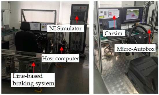
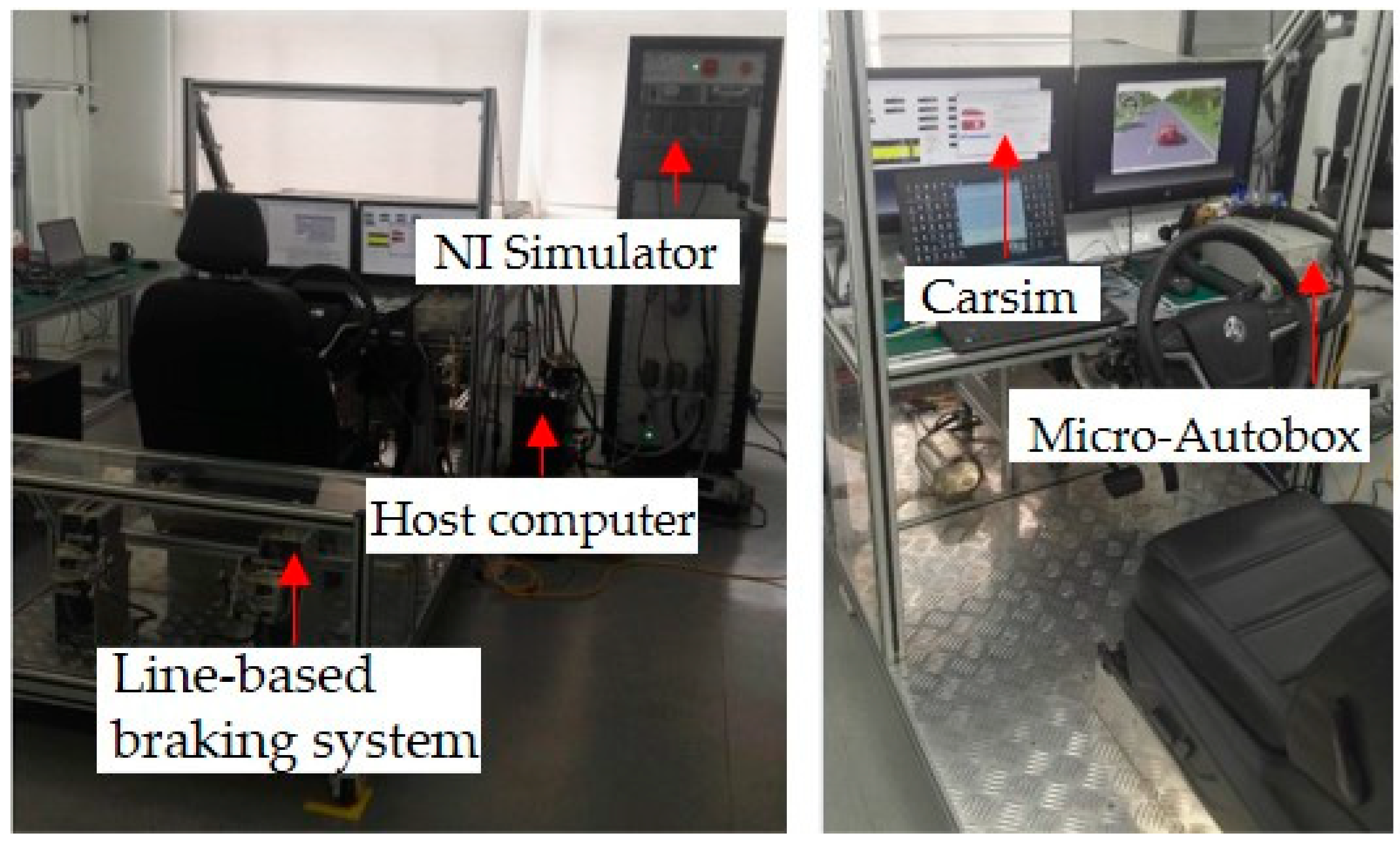
To verify the effectiveness of the control strategy proposed in this paper, a hardware-in-the-loop (HIL) test platform was established, as shown in Figure 5. Figure 5 presents the operational architecture diagram of the HIL test platform, which consists of three components: a rapid prototyping controller, an NI simulator, and simulation scenarios. A vehicle dynamics model was configured in the simulation software CarSim 2021 and downloaded to the NI simulator, enabling the real-time operation of the vehicle dynamics model within the NI simulator. Prescan 2021 was used to construct simulated lane-changing scenarios, and CAN communication with the NI simulator was realized through a CAN analyzer manufactured by Vector, ensuring that the vehicle in the NI simulator achieves accurate dynamic responses under specific scenarios. The control strategy involved in this paper was downloaded to AUTOBOX 2021, a rapid prototyping controller. Two lane-changing conditions were set in Prescan for algorithm verification, namely the double-lane-change scenario and the slalom maneuver scenario.

Figure 5. Hardware-in-the-loop test platform.

To demonstrate the advantages of the control strategy established in this paper, two additional control models are selected for comparison. Specifically, Controller A is defined as the path-tracking and handling stability coordination strategy proposed in this study; Controller B refers to a standalone 4WS (Four-Wheel Steering) controller based on the Nash game; and Controller C denotes a feedforward + feedback path-tracking controller [30]. The parameters of the vehicle and controllers are provided in Table 3.

Table 3. The parameters of the whole vehicle.

Parameter Name	Symbol	Value
Vehicle mass	$m$	1235 kg
Distance from CG to front axle	$a$	1.2 m
Distance from CG to rear axle	$b$	1.35
The peak value of torque	$T_{\max }$	180 Nm
The peak value of power	$P_{\max }$	100 kW
Wheel base	$d$	2.4 m
Maximum rotational speed of the motor	$n_{\max }$	3850 r/min

4.1. Double Lane Change Test on High Adhesion Coefficient Road Surface

The double lane change scenario is selected for verification, where the vehicle speed is set to 90 km/h and the road surface adhesion coefficient is set to 0.85. The simulation results are shown in Figure 6. As depicted in Figure 6a, which presents the trajectory tracking path results, all three control methods can achieve tracking of the desired trajectory. Under the control of Controller A, the deviation between the actual vehicle trajectory and the reference trajectory is the smallest, which is particularly evident at the two lane-changing positions. It can be known from Figure 6b,c that the yaw rate and sideslip angle corresponding to the algorithm proposed in this paper are smaller and have a better convergence trend. Figure 6d shows the phase plane curve. It can be observed that the phase plane curve corresponding to the algorithm proposed in this paper is more uniformly concentrated near the origin, indicating that the algorithm of Controller A has improved the handling stability of the vehicle under the double lane change scenario. Figure 6e,f show the data of the control variable rear wheel and the control variable front wheel, respectively. It can be seen from Figure 6e that the rear wheel steering angle of Controller A is smaller than that of Controller B, which is due to the intervention of the DYC (Direct Yaw Control) system in the control, improving the motion states of the front and rear wheels. Figure 6g,h display the statistical results of lateral errors.

Figure 6. Test results of double lane change working condition on high-adhesion road surface.

It can be observed from the simulation results that the maximum values of the vehicle sideslip angle and yaw rate occur at approximately 4.8 s. Under the three control methods, the variation ranges of the sideslip angle corresponding to Controller A, Controller B, and Controller C are −0.0682 rad to 0.0797 rad, −0.0736 rad to 0.0891 rad, and −0.2083 rad to 0.1374 rad, respectively; while the ranges of the yaw rate are −0.5340 rad/s to 0.4819 rad/s, −0.5764 rad/s to 0.6824 rad/s, and −0.6241 rad/s to 0.8001 rad/s, respectively. In terms of the tracking accuracy of the ideal trajectory, the mean values of lateral displacement deviations are 0.1832 m, 0.2244 m, and 0.2564 m, respectively, with the root mean square (RMS) errors being 0.058 m, 0.0683 m, and 0.1103 m, respectively. For the heading angle, the mean values of deviations are 0.0478 rad, 0.0527 rad, and 0.1101 rad, respectively, and the corresponding RMS errors are 0.0130 rad, 0.0128 rad, and 0.0251 rad, respectively. Compared with Controller B and Controller C, the peak values of the sideslip angle under Controller A are reduced by 10.5% and 67.3%, respectively; meanwhile, the peak values of the yaw rate are decreased by 29.4% and 39.8%, respectively. As shown in Table 4, the simulation results for different control strategies under the double lane change condition on a high-adhesion road surface are compared. The table presents the maximum values of the sideslip angle, yaw rate, and the lateral displacement deviation for each control strategy.

Table 4. Comparison of simulation results for different control strategies under double lane change conditions on high-adhesion road surface.

Control Method	Sideslip Angle (rad)	Yaw Rate (rad/s)	Lateral Displacement Deviation (m)	Root Mean Square (RMS) Error (m)	Heading Angle Deviation (rad)	RMS Error for Heading (rad)
Controller A	−0.0682 to 0.0797	−0.5340 to 0.4819	0.1832	0.0580	0.0478	0.0130
Controller B	−0.0736 to 0.0891	−0.5764 to 0.6824	0.2244	0.0683	0.0527	0.0128
Controller C	−0.2083 to 0.1374	−0.6241 to 0.8001	0.2564	0.1103	0.1101	0.0251

4.2. Double Lane Change Test on Low Adhesion Coefficient Road Surface

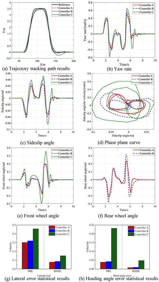
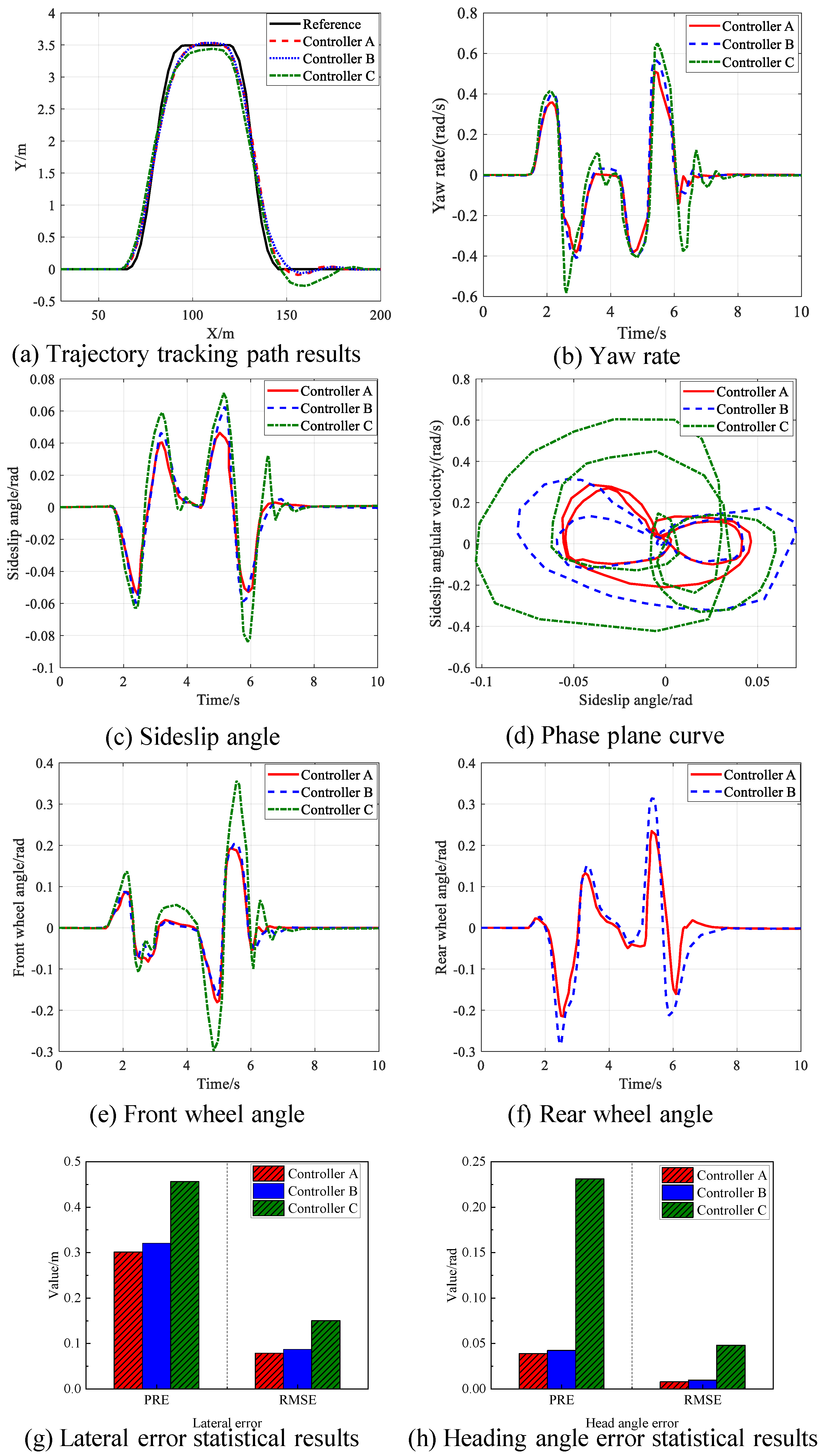
Figure 7 shows the vehicle state data at a vehicle speed of 75 km/h with a road surface adhesion coefficient of 0.3. As can be seen from Figure 7a, the vehicle can track the desired trajectory under all three control methods. However, under the control of the algorithm proposed in this paper, the deviation between the actual trajectory and the reference trajectory is the smallest. Figure 7b–d present the simulation results of handling stability. Both Controller A and Controller B exhibit excellent convergence effects in their stability response curves. Compared with Controller B and Controller C, Controller A reduces the peak values of the sideslip angle by 6.8% and 39.0%, respectively, and the peak values of the yaw rate by 16.2% and 32.5%, respectively. Additionally, the convergence region of the phase trajectory of Controller A is the smallest. It can be observed from Figure 7e,f that the steering angles of the front and rear wheels of the vehicle basically maintain the same steering trend, which improves the driving safety of the vehicle. Meanwhile, Controller A has the smallest rear-wheel steering angle control input. Figure 7g,h show the statistical results of the maximum lateral deviation and heading angle deviation under the three control methods.

Figure 7. Test results of double lane change working condition on low-adhesion road surface.

It can be seen from the simulation results that the maximum values of the vehicle sideslip angle and yaw rate occur at approximately 5.7 s. Under the three control methods, the variation ranges of the sideslip angle corresponding to Controller A, Controller B, and Controller C are −0.0579 rad to 0.0459 rad, −0.0621 rad to 0.0676 rad, and −0.0829 rad to 0.0753 rad, respectively; and the ranges of the yaw rate are −0.3928 rad/s to 0.5010 rad/s, −0.4202 rad/s to 0.5981 rad/s, and −0.5819 rad/s to 0.6582 rad/s, respectively. In terms of the tracking accuracy of the ideal trajectory, the mean values of lateral displacement deviations are 0.3011 m, 0.3211 m, and 0.4562 m, respectively, with the root mean square (RMS) errors being 0.0787 m, 0.0874 m, and 0.1501 m, respectively. The mean values of heading angle deviations are 0.0387 rad, 0.0423 rad, and 0.2310 rad, respectively, and the corresponding RMS errors of the heading angle are 0.0078 rad, 0.0098 rad, and 0.0481 rad, respectively. As shown in Table 5, the simulation results for different control strategies under the double lane change condition on a low-adhesion road surface are compared.

Table 5. Comparison of simulation results for different control strategies under double lane change conditions on low-adhesion road surface.

Control Method	Sideslip Angle (rad)	Yaw Rate (rad/s)	Lateral Displacement Deviation (m)	Root Mean Square (RMS) Error (m)	Heading Angle Deviation (rad)	RMS Error for Heading (rad)
Controller A	−0.0579 to 0.0459	−0.3928 to 0.5010	0.3011	0.0787	0.0387	0.0078
Controller B	−0.0621 to 0.0676	−0.4202 to 0.5981	0.3211	0.0874	0.0423	0.0098
Controller C	−0.0829 to 0.0753	−0.5819 to 0.6582	0.4562	0.1501	0.2310	0.0481

4.3. Slalom Condition Test on Low Adhesion Coefficient Road Surface

The slalom maneuver scenario is mainly designed to verify the vehicle’s stability during continuous obstacle avoidance when the vehicle is traveling at high speeds. The vehicle speed is set to 80 km/h, and the road surface adhesion condition is 0.3. Simulations are conducted under three control methods, and the simulation results are shown in Figure 8. As shown in Figure 8a, all three control methods can effectively track the target path, with the error ranges falling within reasonable limits. Compared with Controller B, the maximum displacement error of Controller A is reduced by 10.8%. However, the maximum displacement error of Model 3 reaches 0.6432 m, indicating the worst path-tracking performance. Figure 8b,c show the yaw rate curve and the sideslip angle curve, respectively. Compared with Controller B and Controller C, Controller A reduces the peak sideslip angle by 17.4% and 38.4%, respectively, and the peak yaw rate by 14.2% and 26.1%, respectively. Figure 8d presents the phase plane curve, from which it can be seen that the stability response curve of Controller A has the best convergence effect. As can be observed from Figure 8e,f, the steering angles of the front and rear wheels of the vehicle basically maintain the same steering trend, which improves the driving safety of the vehicle. Meanwhile, Controller A has the smallest rear-wheel steering angle control input. Figure 8g,h show the statistical results of the maximum lateral deviation and heading angle deviation under the three control methods.

Figure 8. Test results of slalom condition on low-adhesion road surface.

It can be seen from the simulation results that the maximum values of the vehicle sideslip angle and yaw rate appear at approximately 7.6 s. Under the three control methods, the variation ranges of the sideslip angle corresponding to Controller A, Controller B, and Controller C are −0.0521 rad to 0.0496 rad, −0.0633 rad to 0.0621 rad, and −0.0846 rad to 0.0681 rad, respectively; and the ranges of the yaw rate are −0.3291 rad/s to 0.3012 rad/s, −0.3571 rad/s to 0.3505 rad/s, and −0.3842 rad/s to 0.4071 rad/s, respectively. In terms of the tracking accuracy of the ideal trajectory, the mean values of lateral displacement deviations are 0.2011 m, 0.2422 m, and 0.2611 m, respectively, and the root mean square (RMS) errors are 0.0811 m, 0.0911 m, and 0.1362 m, respectively. The mean values of heading angle deviations are 0.0410 rad, 0.0478 rad, and 0.1971 rad, respectively, and the RMS errors of the heading angle are 0.0089 rad, 0.0098 rad, and 0.0397 rad, respectively. Therefore, the path-tracking and handling stability coordinated controller proposed in this paper achieves the highest path-tracking accuracy. As shown in Table 6, the comparison of simulation results for different control strategies under the double lane change condition reveals significant differences in vehicle performance. The table highlights the maximum values of sideslip angle, yaw rate, and lateral displacement deviation, as well as the corresponding RMS errors for lateral displacement and heading angle. These results underscore the advantages of the proposed control strategy in achieving superior path-tracking accuracy and handling stability.

Table 6. Comparison of simulation results for different control strategies under slalom conditions on low-adhesion road surface.

Control Method	Sideslip Angle (rad)	Yaw Rate (rad/s)	Lateral Displacement Deviation (m)	Root Mean Square (RMS) Error (m)	Heading Angle Deviation (rad)	RMS Error for Heading (rad)
Controller A	−0.0521 to 0.0496	−0.3291 to 0.3012	0.2011	0.0811	0.0410	0.0089
Controller B	−0.0633 to 0.0621	−0.3571 to 0.3505	0.2422	0.0911	0.0478	0.0098
Controller C	−0.0846 to 0.0681	−0.3842 to 0.4071	0.2611	0.1362	0.1971	0.0397

4.4. Slalom Condition Test on High Adhesion Coefficient Road Surface

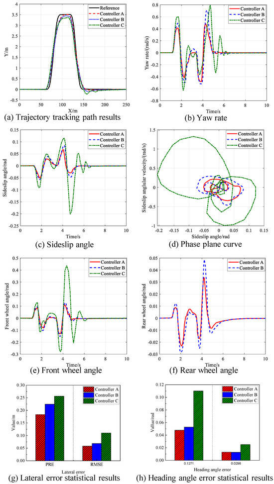
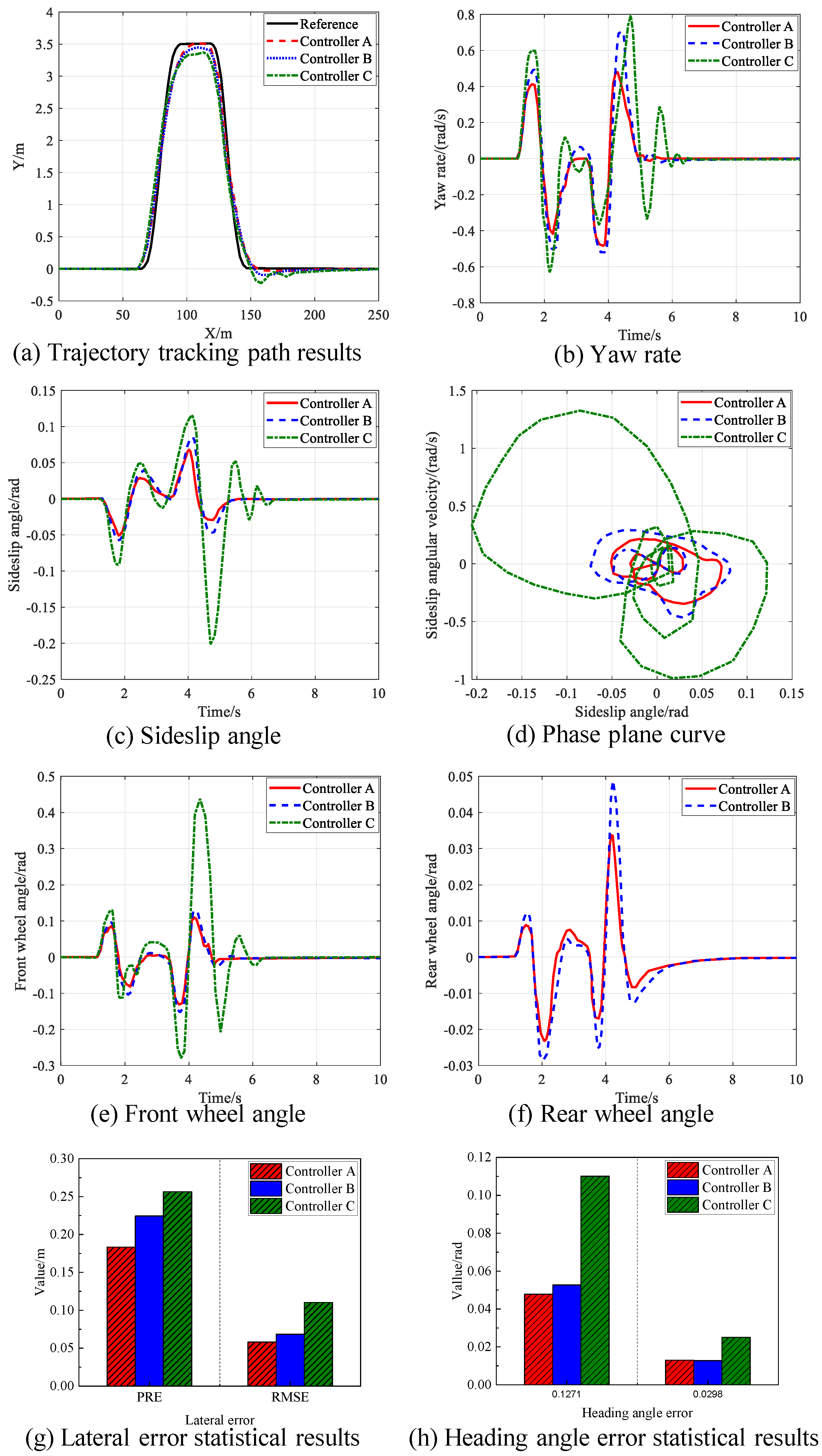
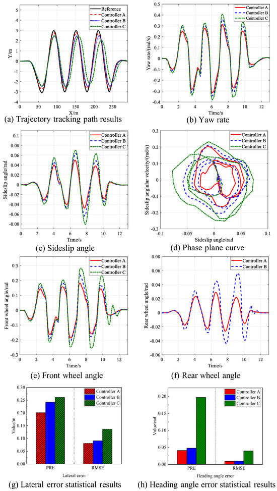
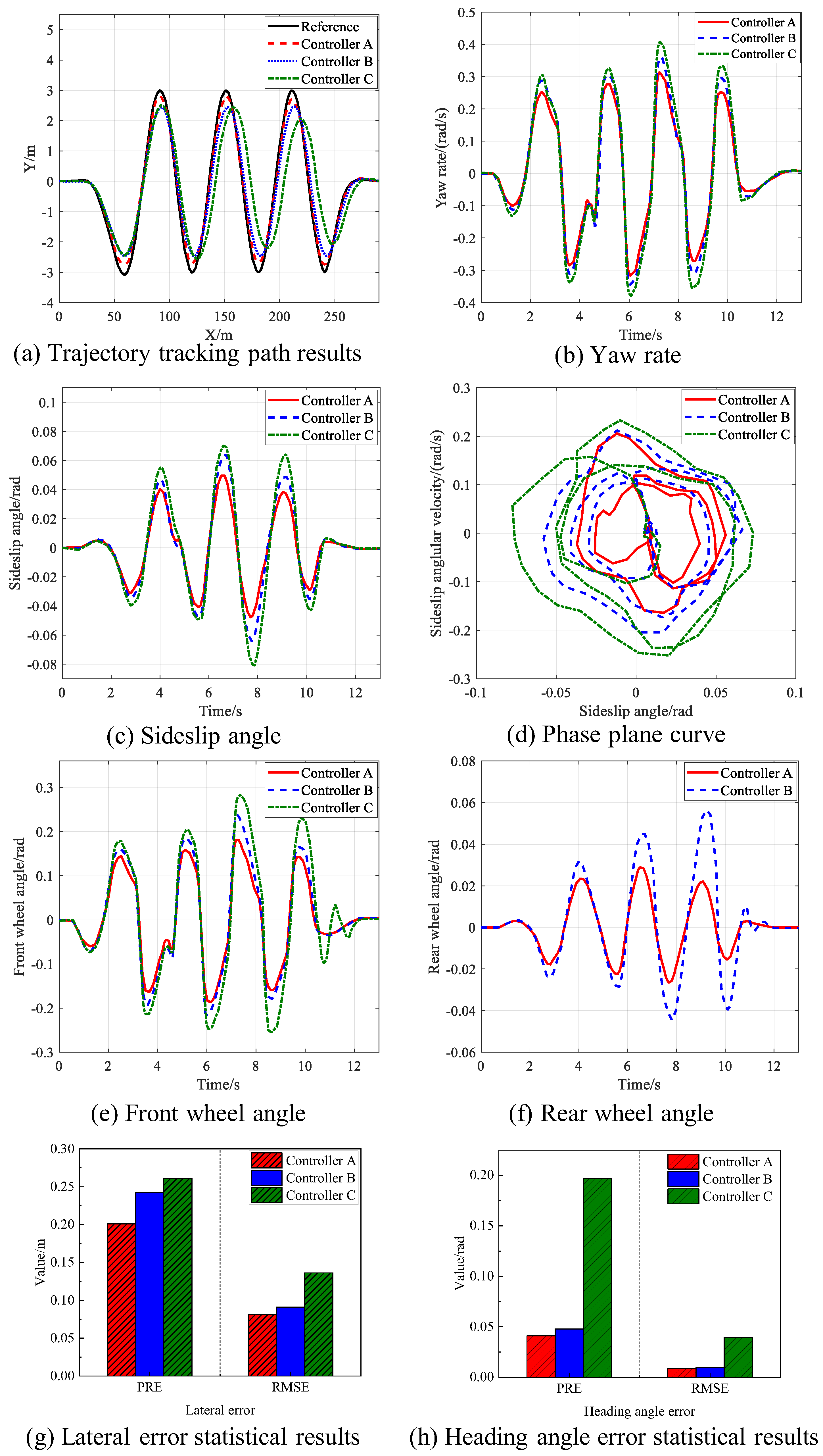
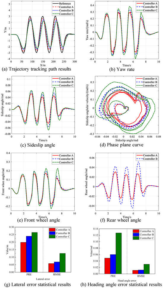
In this working condition, the vehicle speed is set to 90 km/h, and the road surface adhesion coefficient is set to 0.8. The simulation results are shown in Figure 9. As presented in Figure 9a, which illustrates the trajectory tracking path results, all three control methods can achieve the tracking of the desired trajectory. Under the control of Controller A, the deviation between the actual vehicle trajectory and the reference trajectory is the smallest. It can be seen from Figure 9b,c that the yaw rate and sideslip angle corresponding to the algorithm proposed in this paper are smaller and show a favorable convergence trend. Figure 9d displays the phase plane curve. It is evident that the phase plane curve corresponding to the proposed algorithm is more uniformly concentrated near the origin, indicating that the algorithm of Controller A has improved vehicle handling stability. Figure 9e,f show the data of the control variable (rear wheel) and the control variable (front wheel), respectively. It can be observed from Figure 9e that the rear wheel steering angle of Controller A is smaller than that of Controller B, which demonstrates that the method proposed in this paper has improved the motion states of the front and rear wheels. Figure 9g,h present the statistical results of lateral errors.

Figure 9. Test results of slalom condition on high-adhesion road surface.

It can be observed from the simulation results that the maximum values of the vehicle sideslip angle and yaw rate occur at approximately 6.2 s. Under the three control methods, the variation ranges of the sideslip angle corresponding to Controller A, Controller B, and Controller C are −0.0436 rad to 0.0521 rad, −0.0593 rad to 0.0589 rad, and −0.0663 rad to 0.0764 rad, respectively; while the ranges of the yaw rate are −0.3264 rad/s to 0.3011 rad/s, −0.3593 rad/s to 0.3265 rad/s, and −0.3905 rad/s to 0.3571 rad/s, respectively. In terms of the tracking accuracy of the ideal trajectory, the mean values of lateral displacement deviations are 0.1988 m, 0.2396 m, and 0.2645 m, respectively, with the root mean square (RMS) errors being 0.0581 m, 0.0689 m, and 0.1254 m, respectively. For the heading angle, the mean values of deviations are 0.0489 rad, 0.0601 rad, and 0.1271 rad, respectively, and the corresponding RMS errors of the heading angle are 0.0110 rad, 0.0123 rad, and 0.0298 rad, respectively. Compared with Controller B and Controller C, the peak values of the sideslip angle under Controller A are reduced by 26.5% and 34.2%, respectively, and the peak values of the yaw rate are decreased by 7.8% and 16.4%, respectively. As shown in Table 7, the simulation results for different control strategies under the double lane change condition on a high-adhesion road surface are compared. The table presents the maximum values of the sideslip angle, yaw rate, and the lateral displacement deviation for each control strategy, along with the corresponding root mean square (RMS) errors for lateral displacement and heading angle.

Table 7. Comparison of simulation results for different control strategies under slalom conditions on high-adhesion road surface.

Control Method	Sideslip Angle (rad)	Yaw Rate (rad/s)	Lateral Displacement Deviation (m)	Root Mean Square (RMS) Error (m)	Heading Angle Deviation (rad)	RMS Error for Heading (rad)
Controller A	−0.0436 to 0.0521	−0.3264 to 0.3011	0.1988	0.0581	0.0489	0.0110
Controller B	−0.0593 to 0.0589	−0.3593 to 0.3265	0.2396	0.0689	0.0601	0.0123
Controller C	−0.0663 to 0.0764	−0.3905 to 0.3571	0.2645	0.1254	0.1271	0.0298

5. Conclusions

This paper establishes a 4WS and DYC coordinated control strategy for in-wheel motor-driven electric vehicles to address the challenges of path-tracking performance and handling stability under extreme working conditions. The following conclusions are drawn:

(1)

Based on the shared steering model, a 4WS controller is designed using the Nash game, which fully considers the interaction between AFS and ARS.

(2)

The coordinated controller integrated with DYC effectively utilizes the respective advantages of the 4WS and DYC systems, further enhancing the handling stability of the vehicle during path tracking.

(3)

Tests under double-lane-change and slalom working conditions were carried out using a hardware-in-the-loop test platform. The results showed that under high-adhesion road conditions, the proposed control strategy reduced the peak values of the vehicle’s centroid sideslip angle by 17.4% and 38.4%, respectively, and the peak values of the yaw rate by 14.2% and 26.1%, respectively. Under low-adhesion road conditions, the proposed strategy reduced the peak values of the sideslip angle and the yaw rate significantly compared to other control strategies.

6. Limitations and Future Work

While the proposed strategy has shown promising results, several limitations exist. The model assumes constant road adhesion, which may not hold true in all real-world conditions. Future work will consider incorporating adaptive methods to handle variations in road conditions. Additionally, an extension of the finite-time sliding surface (used in Equation (22) to a fixed-time controller, which offers better robustness and faster convergence, could be explored in future studies. A comparison with fixed-time control methods, such as those discussed by Polyakov (2012) [31] and Ning et al. (2019) [32], will help highlight the differences and advantages of the proposed approach.

Furthermore, the parameter sensitivity of the system and possible extensions to rule-free adherence estimation and coordination will be investigated to improve the adaptability of the control system in dynamic environments.

References

- Wang, H.; Huang, Y.; Khajepour, A.; Cao, D.; Lv, C. Ethical decision-making platform in autonomous vehicles with lexicographic optimization based model predictive controller. IEEE Trans. Veh. Technol. 2020, 69, 8164–8175. [Google Scholar] [CrossRef] [Scilit]
- Christ, F.; Wischnewski, A.; Heilmeier, A.; Lohmann, B. Time-optimal trajectory planning for a race car considering variable tyre-road friction coefficients. Veh. Syst. Dyn. 2021, 59, 588–612. [Google Scholar] [CrossRef] [Scilit]
- Sano, S.; Furukawa, Y.; Shiraishi, S. Four wheel steering system with rear wheel steer angle controlled as a function of steering wheel angle. SAE Trans. 1986, 95, 880–893. [Google Scholar]
- Russell, H.E.B.; Gerdes, J.C. Design of variable vehicle handling characteristics using four wheel steer-by-wire. IEEE Trans. Control Syst. Technol. 2016, 24, 1529–1540. [Google Scholar] [CrossRef] [Scilit]
- Hiraoka, T.; Nishihara, O.; Kumamoto, H. Automatic path-tracking controller of a four-wheel steering vehicle. Veh. Syst. Dyn. 2009, 47, 1205–1227. [Google Scholar] [CrossRef] [Scilit]
- Chatzikomis, C.I.; Spentzas, K.N. Comparison of a vehicle equipped with electronic stability control to a vehicle with four wheel steering(4WS). Forsch. Im Ingenieurwesen 2014, 78, 13–25. [Google Scholar] [CrossRef] [Scilit]
- Gao, L.; Jin, L.; Zheng, Y.; Li, K.Y. Design of radial basis function neural network compound controller for four wheel steering vehicle. J. Jilin Univ. 2016, 46, 366–372. [Google Scholar]
- Xie, X.Y.; Jin, L.S.; Gao, L.L.; Xia, H.P. Study on rear wheel active steering control based on variable weight coefficient of LQR. J. Zhejiang Univ. (Eng. Sci.) 2018, 52, 446–452. [Google Scholar]
- Meng, Q.; Sun, Z.Y.; Li, Y. Finite-time controller design for four-wheel-steering of electric vehicle driven by four in-wheel motors. Int. J. Control Autom. Syst. 2018, 16, 1814–1823. [Google Scholar] [CrossRef] [Scilit]
- Shi, K.; Yuan, X.; He, Q. Double-layer dynamic decoupling control system for the yaw stability of four-wheel steering vehicle. Int. J. Control Autom. Syst. 2019, 17, 1255–1263. [Google Scholar] [CrossRef] [Scilit]
- Yu, S.; Tan, L.; Wang, W.; Chen, H. Control of active four-wheel steering vehicle based on triple-step method. J. Jilin Univ. (Eng. Technol. Ed.) 2019, 49, 934–942. (In Chinese) [Google Scholar]
- Yin, H.; Zhao, C.; Li, M.; Ma, C.; Chow, M.Y. A game theory approach to energy management of an engine-generator/battery/ultracapacitor hybrid energy system. IEEE Trans. Ind. Electron. 2016, 63, 4266–4277. [Google Scholar] [CrossRef] [Scilit]
- Na, X.; Cole, D.J. Game-theoretic modeling of the steering interaction between a human driver and a vehicle collision avoidance controller. IEEE Trans. Hum. -Mach. Syst. 2015, 45, 25–38. [Google Scholar] [CrossRef] [Scilit]
- He, Y.L.; Ma, J.; Yang, S.K.; Zheng, W.; Xue, Q.F. Research on stability model predictive control of intelligent electric vehicle with preview characteristics. Automot. Eng. 2023, 45, 719–734. [Google Scholar]
- Lin, C.; Liang, S.; Gong, X.L. Integrated dynamic control strategy for extreme maneuvers of 4WIDEVs. Automot. Eng. 2022, 44, 1372–1385. [Google Scholar]
- Zong, C.; Zheng, H.; Tian, C.; Pan, Z.; Dong, Y.; Yuan, D. Vehicle stability control strategy based on direct yaw moment control. J. Jilin Univ. (Eng. Technol. Ed.) 2008, 5, 1010–1014. [Google Scholar]
- Guo, H.; Liu, F.; Xu, F.; Chen, H.; Cao, D.; Ji, Y. Nonlinear model predictive lateral stability control of active chassis for intelligent vehicles and its FPGA implementation. IEEE Trans. Syst. Man Cybern. Syst. 2019, 49, 1–13. [Google Scholar] [CrossRef] [Scilit]
- Guo, N.; Lenzo, B.; Zhang, X.; Zou, Y.; Zhai, R.; Zhang, T. A real-time nonlinear model predictive controller for yaw motion optimization of distributed drive electric vehicles. IEEE Trans. Veh. Technol. 2020, 69, 4935–4946. [Google Scholar] [CrossRef] [Scilit]
- Pacejka, H.B.; Bakker, E. The Magic Formula Tyre Model. Veh. Syst. Dyn. 1993, 19, 1–20. [Google Scholar] [CrossRef] [Scilit]
- Bakker, E.; Pacejka, H.B. Tyre modelling for use in vehicle dynamics simulations. Veh. Syst. Dyn. 1991, 20, 281–296. [Google Scholar]
- Liu, X.; Wang, L. Vehicle Dynamic Control Based on a Tire Force Model with Magic Formula. Int. J. Automot. Technol. 2011, 12, 519–526. [Google Scholar]
- Demirci, M.; Gokasan, M. Adaptive optimal control allocation using Lagrangian neural networks for stability control of a 4WS-4WD electric vehicle. Trans. Inst. Meas. Control 2013, 35, 1139–1151. [Google Scholar] [CrossRef] [Scilit]
- Li, B.; Rakheja, S.; Feng, Y. Enhancement of vehicle stability through integration of direct yaw moment and active rear steering. Proc. Inst. Mech. Eng. Part D J. Automob. Eng. 2016, 230, 830–840. [Google Scholar] [CrossRef] [Scilit]
- Yong, J.; Gao, F.; Ding, N.; He, Y. An integrated algorithm for vehicle stability improvement with the coordination of direct yaw moment and four-wheel steering control. Int. J. Veh. Des. 2017, 74, 231–256. [Google Scholar] [CrossRef] [Scilit]
- Song, J. Integrated vehicle dynamic controls using active rear wheel steering and four-wheel braking. Int. J. Veh. Syst. Model. Test. 2018, 13, 26–43. [Google Scholar] [CrossRef] [Scilit]
- Alimorad, H. An iterative method and maximal solution of Coupled algebraic Riccati equations. J. Algorithms Comput. 2022, 54, 109–123. [Google Scholar]
- Wang, Y.; Chen, G.; Jiang, H.; Zhou, J.; Zhang, T.; Zhou, G.; Wang, C.; Zhao, W. Coordination Control for Path Tracking and Stability of 4WS-4WID Automated Vehicles: A Game Theory-Based Approach. IEEE Trans. Veh. Technol. 2025, 74, 7392–7403. [Google Scholar] [CrossRef] [Scilit]
- Chen, J.; Shuai, Z.; Zhang, H.; Zhao, W. Path following control of autonomous four-wheel-independent-drive electric vehicles via second-order sliding mode and nonlinear disturbance observer techniques. IEEE Trans. Ind. Electron. 2021, 68, 2460–2469. [Google Scholar] [CrossRef] [Scilit]
- Huang, Y.; Xie, Y.; Huang, W. Complementary Sliding Mode Speed Control with Saturation Function Boundary Layer Optimization. J. Harbin Inst. Technol. (New Ser.) 2019, 26, 67–71. [Google Scholar]
- Liu, G.; Shao, W. Coordinated Control Strategy for Stability Control and Trajectory Tracking with Wheel-Driven Autonomous Vehicles Under Harsh Situations. World Electr. Veh. J. 2025, 16, 163. [Google Scholar] [CrossRef] [Scilit]
- Polyakov, A. Nonlinear feedback design for fixed-time stabilization of linear control systems. IEEE Trans. Autom. Control 2012, 57, 2106–2110. [Google Scholar] [CrossRef] [Scilit]
- Ning, B.; Han, Q.L. Prescribed finite-time consensus tracking for multi-agent systems with nonholonomic chained-form dynamics. IEEE Trans. Autom. Control 2019, 64, 1686–1693. [Google Scholar] [CrossRef] [Scilit]
Disclaimer/Publisher’s Note: The statements, opinions and data contained in all publications are solely those of the individual author(s) and contributor(s) and not of MDPI and/or the editor(s). MDPI and/or the editor(s) disclaim responsibility for any injury to people or property resulting from any ideas, methods, instructions or products referred to in the content. |
© 2025 by the author. Licensee MDPI, Basel, Switzerland. This article is an open access article distributed under the terms and conditions of the Creative Commons Attribution (CC BY) license (https://creativecommons.org/licenses/by/4.0/).