Design and Implementation of Decoupling Controllers for Vertical Suspension System of Magnetic Suspension and Balance System

Abstract

The Magnetic Suspension Balance System (MSBS) serves as a core apparatus for interference-free aerodynamic testing in wind tunnels, where its high-precision levitation control performance directly determines the reliability of aerodynamic force measurements. This paper addresses the strong coupling issues induced by rigid-body motion in the MSBS vertical suspension system and proposes a decoupling control framework integrating classical decoupling methods with geometric feature transformation. First, a nonlinear dynamic model of the six-degree-of-freedom MSBS is established. Through linearization analysis of the vertical suspension system, the intrinsic mechanism of displacement-pitch coupling is revealed. Building upon this foundation, a state feedback decoupling controller is designed to achieve decoupling among dynamic channels. Simulation results demonstrate favorable control performance under ideal linear conditions. To further overcome its dependency on model parameters, a decoupling strategy based on geometric feature transformation is proposed, which significantly enhances system robustness in nonlinear operating conditions through state-space reconstruction. Finally, the effectiveness of the proposed method in vertical suspension control is validated through both numerical simulations and a physical MSBS experimental platform.

1. Introduction

Wind tunnels represent critical ground-based simulation facilities, providing indispensable data support for aircraft aerodynamic design and performance evaluation [1]. Unlike traditional wind tunnel testing techniques employing mechanical supports and strain-gauge balances, MSBS constitutes a breakthrough contactless support and measurement technology [2]. The fundamental principle involves utilizing actively closed-loop controlled electromagnetic forces to apply precise suspension forces to test models incorporating permanent magnets or ferromagnetic structures. This enables stable levitation of model within the wind tunnel test section flow field without mechanical contact [3,4]. Simultaneously, the system computes aerodynamic forces and moments acting on the suspension model by real-time monitoring of driving coil currents and six-degree-of-freedom position and orientation data of the suspension model [5,6,7]. The MSBS completely eliminates mechanical support structures, thereby fundamentally removing physical flow-field interference caused by support struts. This technology offers a promising pathway for acquiring high-fidelity aerodynamic test data [8,9].

The development of high-performance controllers is essential for the engineering application of MSBS, enabling stable model suspension in strongly disturbed flows [10]. Existing research has primarily focused on decentralized control architectures. Various control strategies have been explored, including independent PD controllers for each degree of freedom [11], PID control applied to magnetically suspended re-entry vehicle models [12], IFT adaptive control [13], and PI controllers for error elimination [14]. Some studies have specifically addressed decoupling challenges, proposing methods such as feedforward control with decoupling scaling factors [15]. Other notable contributions include a high-frequency synchronous PI control system that improved response times [16], a dual-loop digital controller for enhanced stability [17], and an FTD-based algorithm for noise suppression [18].

Despite these advancements, decentralized control remains predominant. This approach faces fundamental limitations in systems like the high-aspect-ratio missile-type configuration studied herein, which differs significantly from re-entry vehicle models investigated by NASA Langley Research Center and Old Dominion University [19,20,21]. The elongated geometry creates substantial offsets between electromagnetic force application points and the center of mass, inducing strong translational-rotational coupling that can provoke destabilizing oscillations without precise compensation. Although decoupling strategies have been proposed [14], research specifically addressing five-pair coil MSBS configurations under strong coupling conditions remains limited. Therefore, advancing research on coupled dynamic modeling and decoupling control for high-aspect-ratio missile-type models in MSBS is of both significant theoretical importance and practical engineering value.

Based on the observations above, this paper addresses the vertical suspension control of a MSBS by adopting a six-degree-of-freedom dynamic modeling, analysis, and decoupling control approach for a high-aspect-ratio missile-type model. Main contributions of this paper are as follows:

(1)

For the MSBS applied to high-aspect-ratio missile configurations, a six-degree-of-freedom dynamic model is established. Taking the vertical suspension system as an example, linearization-based analysis reveals the inherent translational-rotational coupling mechanism caused by the deviation between electromagnetic force application points and the model’s center of mass.

(2)

A model-based feedback decoupling controller is designed and evaluated specifically for the vertical suspension system. Both simulation and experimental results demonstrate that this method exhibits high sensitivity to parameter variations, revealing its fundamental limitation of insufficient robustness in practical MSBS applications.

(3)

A decoupling control strategy based on geometric feature transformation is proposed. This method eliminates the dependency on precise system parameters and demonstrates effective decoupling performance through comparative simulations and experimental validation on an actual MSBS.

The paper structure is as follows: Section 2 describes the MSBS, establishes the six-degree-of-freedom dynamic model, and presents the linearization process. Section 3 analyzes coupling mechanisms and presents the feedback decoupling controller alongside the geometric-feature-transformation-based decoupling control strategy. Section 4 details simulation and experimental validation. Section 5 summarizes conclusions and outlines directions for future work.

2. System Modeling and Linearization

2.1. MSBS Description and Six-Degree-of-Freedom Dynamic Equations

The MSBS comprises electromagnetic coils, a connecting frame, a controller, a position sensor system, and a model with embedded cylindrical magnets. The system structure is illustrated in Figure 1. The coil system consists of eight electromagnets (#1 to #8) and two solenoids (#0 and #9), arranged in a point-symmetrical distribution centered at the origin of the test section [18]. A right-handed Cartesian coordinate system is fixed relative to the wind tunnel. The origin of this coordinate system is defined at the reference center (typically the center of mass of the test model) [22]. The positive x-axis is aligned with the freestream flow direction, the y-axis lies in the horizontal plane perpendicular to the x-axis, and the z-axis completes the right-handed system by pointing vertically upward.

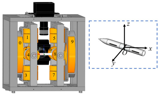
Figure 1. Schematic diagram of the MSBS structure and coordinate system.

In the MSBS, the electromagnetic array achieves precise control over the six-degree-of-freedom motion of the magnetically suspended model through the application of three-dimensional electromagnetic forces and moments. The electromagnetic force components are defined as follows: the axial force along the wind tunnel axis, the vertical force in the vertical direction, and the lateral force in the horizontal transverse direction. The electromagnetic moment components include the pitching moment, yawing moment and rolling moment. The specific current combinations required to generate these forces and moments are summarized in Table 1.

Table 1. Coil current combinations.

Form of Resultant Force	Current Combination	Form of Resultant Force	Current Combination
Axial force	$\left(I_0+I_9\right)$	Pitching moment	$\left(I_1+I_3-I_5-I_7\right)$
Vertical force	$\left(I_1+I_3+I_5+I_7\right)$	Yawing moment	$\left(I_2+I_4-I_6-I_8\right)$
Lateral force	$\left(I_2+I_4+I_6+I_8\right)$	Rolling moment	$-\left(I_2-I_4+I_6-I_8\right)$

Note: $I_0$ to $I_9$ represent the currents passing through electromagnets 0 to 9, respectively.

The position and attitude sensor system employs optical position sensors integrated with five high-resolution CCD linear array sensors [23]. As shown in Figure 2, CCD linear array sensors capture images of the model illuminated by LED light sources. Model position and orientation are derived by detecting model edges and marker boundaries.

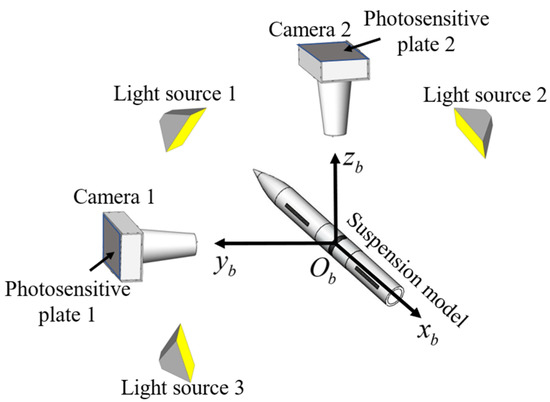
Figure 2. Position and attitude sensor system (where $O_b-x_b{y}_b{z}_b$ is body coordinate system).

The magnetic excitation array of the MSBS is primarily configured at the nose and tail sections of the suspension model. Spatial magnetic flux density distributions exhibit significantly higher field strength near the suspension model ends compared to the mid-section. This non-uniform field distribution allows simplification of the electromagnetic resultant force into concentrated forces acting at the suspension model nose and tail. Simultaneously, the gravitational vector acts at the suspension model center of mass. Additionally, spatial electromagnetic fields generated by excitation coils induce restoring moments on the suspension model.

As shown in Figure 3, the suspension model of MSBS can be treated as a lightweight rigid rod with specific moments of inertia. This equivalent model provides a simplified basis for analyzing six-degree-of-freedom motion (particularly translation-rotation coupling). The differential equations for six-degree-of-freedom motion are expressed as:

$$\left\{\begin{array}{l}m{\displaystyle \frac{\mathrm{d}{V}_{\mathrm{model}}}{\mathrm{d}t}}=F_{\mathrm{total}}\\ {\displaystyle \frac{\mathrm{d}{H}_{\mathrm{model}}}{\mathrm{d}t}}+{\omega }_x\times H_{\mathrm{model}}=T_{\mathrm{model}}\end{array}\right.$$

(1)

where $V_{\mathrm{model}}$ is the velocity of the suspension model, ${\omega }_x$ is the angular velocity about the x-axis in the rotating coordinate system, and $H_{\mathrm{model}}$ is the angular momentum of the rotor about the center of mass. $F_{\mathrm{total}}$ and $T_{\mathrm{model}}$ are the total external force and moment acting on the magnetically suspension model, respectively.

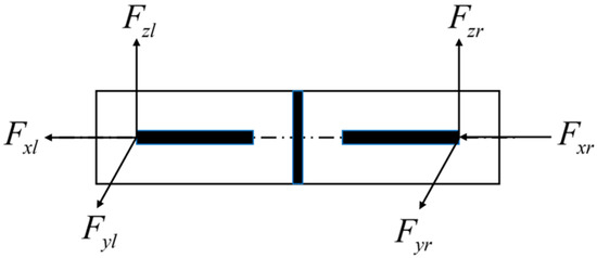
Figure 3. Schematic of force acting on the suspension model (where $F_{xl}$, $F_{yl}$, $F_{zl}$ are the external forces on the front/left end. $F_{xr}$, $F_{yr}$, and $F_{zr}$ are the external forces on the rear/right end of the model).

Constructing the dynamic model of the suspension model requires analyzing its force state along three axes. In the vertical degree of freedom, the model is governed by gravity and the vertical resultant force generated by the front and rear vertical electromagnets. The lateral degree of freedom is dominated by the resultant force from the front and rear lateral electromagnetic actuators. The axial degree of freedom is influenced by both the resultant force from the front and rear axial electromagnetic actuators and aerodynamic disturbances. To achieve accurate control modeling of the model in the absolute coordinate system, the force balance relationship must be transformed into this coordinate system. This coordinate transformation ultimately leads to the differential equations characterizing the translational motion of the model:

$$\left\{\begin{array}{l}m{\ddot{x}}_o=F_{x\_total}\\ m{\ddot{y}}_o=F_{y\_total}\\ m{\ddot{z}}_o=F_{z\_total}\end{array}\right.$$

(2)

where $x_o$, $y_o$ and $z_o$ are the coordinates of the center of mass of the magnetically suspension model along the $x$, $y$, and $z$ axes in the absolute coordinate system. $F_{x\_total}$, $F_{y\_total}$, $F_{z\_total}$ are the resultant forces acting on the model along the $x$, $y$, and $z$ axes, respectively. The expressions for the resultant forces along each axis are as follows:

$$\left\{\begin{array}{l}{F}_{x\_total}=F_{e,0}+F_{e,9}+F_D\\ F_{y\_total}=F_{e,2}+F_{e,4}+F_{e,6}+F_{e,8}-F_Y\\ F_{z\_total}=F_{e,1}+F_{e,3}+F_{e,5}+F_{e,7}+F_L-mg\end{array}\right.$$

(3)

where $F_{e,i},i=0,1,\dots ,9$ represents the electromagnetic force exerted by the i-th electromagnet on the model, $F_D$ is the drag force experienced by the model in the flow field, $F_Y$ is the side force, and $F_L$ is the lift force.

By projecting the rotational equations from (1) into the body-fixed coordinate system, the rotational equations in the absolute coordinate system are obtained as:

$$\left\{\begin{array}{l}{J}_x\ddot{\varphi }=T_x\\ J_z\ddot{\psi }-J_x\dot{\varphi }\dot{\theta }=T_y\\ J_y\ddot{\theta }+J_x\dot{\varphi }\dot{\psi }=T_z\end{array}\right.$$

(4)

where $J_x$, $J_y$, $J_z$ are the moments of inertia about the x, y, and z axes, respectively. $\theta$ is the pitch angle of the magnetically suspension model, $\psi$ is the yaw angle, and $\varphi$ is the roll angle. $T_x$, $T_y$, and $T_z$ are the resultant moments about the x, y, and z axes, respectively.

2.2. Linearization of Vertical Dynamics Equations

Ignoring the additional moment generated by the electromagnetic coils on the magnetically suspension model, it can be observed that the angular rate of the model about the x-axis couples the rotational motions of the y and z axes, causing the lateral moment to induce dynamic responses in the orthogonal direction. Since the roll degree of freedom is released during suspension and the roll angular velocity is very small [24], it can be assumed that $\dot{\varphi }\approx 0$. Therefore, the terms $J_x\dot{\varphi }\dot{\psi }$ and $J_x\dot{\varphi }\dot{\theta }$ in the equations can be neglected, meaning that the rotational motions about the y and z axes are decoupled from each other. The vertical dynamics equations can thus be further simplified as follows:

$$z:\left\{\begin{array}{l}m{\ddot{z}}_o=F_{e,1}+F_{e,3}+F_{e,5}+F_{e,7}-mg\\ J_y\ddot{\theta }=(F_{e,1}+F_{e,3}-F_{e,5}-F_{e,7}){\displaystyle \frac{L_{\mathrm{per}}}{2}}\end{array}\right.$$

(5)

where $L_{\mathrm{per}}$ is the length of the embedded permanent magnet.

When the center of the embedded permanent magnet rod is located at $\left(x_{e1},0,z_{e1}\right)$, the electromagnetic force acting on the model is given by:

$$\begin{array}{ll}{F}_{e,1}& =k_{m1}{I}_1\left(3z_{e1}^2{\left(z_{e1}^2+{\left(x_{e1}+L_{\mathrm{per}}/2\right)}^2\right)}^{-{\displaystyle \frac{5}{2}}}-{\left(z_{e1}^2+{\left(x_{e1}+L_{\mathrm{per}}/2\right)}^2\right)}^{-{\displaystyle \frac{3}{2}}}\right.\\ & \left.-3z_{e1}^2{\left(z_{e1}^2+{\left(x_{e1}-L_{\mathrm{per}}/2\right)}^2\right)}^{-{\displaystyle \frac{5}{2}}}+{\left(z_{e1}^2+{\left(x_{e1}-L_{\mathrm{per}}/2\right)}^2\right)}^{-{\displaystyle \frac{3}{2}}}\right)\\ & =k_{m1}{I}_{1}G(z_{e1})\end{array}$$

(6)

where $k_{m1}$ is the electromagnetic force coefficient of electromagnet 1, and $G(z_{e1})$ is an auxiliary function of $z_{e1}$.

Under static suspension conditions, it is assumed that the center of mass of the model fluctuates within a small range near $x_{e1}$. Thus, $\left(x_{e1}+L_{\mathrm{per}}/2\right)$ and $\left(x_{e1}-L_{\mathrm{per}}/2\right)$ can be regarded as constants, and their influence on the vertical electromagnetic force acting on the model can be neglected. The electromagnetic force $F_{e,1}$ is linearized at the equilibrium point $z_{e1}=z_1$, $I_1=I_{v1}$:

$$\begin{array}{ll}{F}_{e,1}& \approx k_{m1}{I}_{v1}G(z_1)+k_{m1}G(z_1)(I_1-I_{v1})+k_{m1}{I}_{v1}{\left.{\displaystyle \frac{\mathit{\partial }G}{\mathit{\partial }{z}_{e1}}}\right|}_{z_1}(z_{e1}-z_1)\\ & =k_{m1}G(z_1)I_1+k_{m1}{G}^{\prime }\left(z_1\right)I_{v1}(z_{e1}-z_1)\end{array}$$

(7)

where $G^{\prime }\left(z_1\right)$ is the partial derivative of $G(z_{e1})$ with respect to $z_{e1}$ evaluated at the equilibrium point $z_{e1}=z_1$, and $I_{v1}$ is the current flowing through electromagnet 1 at the equilibrium point.

Similarly, the linearized expression of the electromagnetic force exerted by electromagnet 3 on the model at the equilibrium point $\left(z_3,I_{v3}\right)$ is:

$$F_{e,3}\approx k_{m3}G(z_3)I_3+k_{m3}{G}^{\prime }\left(z_3\right)I_{v3}(z_{e3}-z_3)$$

(8)

where $k_{m3}$ denotes the electromagnetic force coefficient of Electromagnet 3, and $I_{v3}$ represents the current through Electromagnet 3 at the equilibrium point.

Assuming the distance between the outer surface of the core of electromagnet 1 and the x-axis of the absolute coordinate system is $L_{\mathrm{v}}$, it can be obtained that $z_3=2L_{\mathrm{v}}-z_1$, $I_1=I_3=I_{\mathrm{vf}}$, and $I_{v3}=I_{v1}={\overline{I}}_{\mathrm{vf}}$. Therefore, the total electromagnetic force acting on the front end of the model along the vertical direction, $F_{e,13}$, is:

$$\begin{array}{ll}{F}_{e,13}& =F_{e,1}+F_{e,3}\\ & =k_{\mathrm{vfi}}{I}_{\mathrm{vf}}+k_{\mathrm{vfz}}(z_1-z_{e1})\end{array}$$

(9)

where $k_{\mathrm{vfi}}$ and $k_{\mathrm{vfz}}$ correspond to the current stiffness and positional stiffness of the front vertical segment, respectively.

Following the same linearization procedure, the electromagnetic force acting on the rear vertical segment of the model, $F_{e,57}$, is derived as:

$$F_{e,57}=k_{\mathrm{vbi}}{I}_{\mathrm{vb}}+k_{\mathrm{vbz}}(z_5-z_{e5})$$

(10)

where $k_{\mathrm{vbi}}$ and $k_{\mathrm{vbz}}$ are the current stiffness and positional stiffness of the front vertical segment, respectively, and $I_{\mathrm{vb}}=I_5=I_7$ holds. Under static suspension conditions in the absence of flow, the boundary conditions satisfy:

$$k_{\mathrm{vfz}}{z}_1=k_{\mathrm{vbz}}{z}_5=mg/2$$

(11)

Thus, introducing the linearized electromagnetic forces given by Equations (9) and (10) into the system of Equation (5) yields:

$$z:\left\{\begin{array}{l}m{\ddot{z}}_o=k_{\mathrm{vfi}}{I}_{\mathrm{vf}}-k_{\mathrm{vfz}}{z}_{e1}+k_{\mathrm{vbi}}{I}_{\mathrm{vb}}-k_{\mathrm{vbz}}{z}_{e5}\\ J_y\ddot{\theta }=(k_{\mathrm{vfi}}{I}_{\mathrm{vf}}-k_{\mathrm{vfz}}{z}_{e1}-k_{\mathrm{vbi}}{I}_{\mathrm{vb}}+k_{\mathrm{vbz}}{z}_{e5}){\displaystyle \frac{L_{\mathrm{per}}}{2}}\end{array}\right.$$

(12)

3. Design of the Decoupling Controller for Vertical Suspension System

3.1. Coupling Term Analysis

Based on the rigid-body properties of the magnetically suspension model, it is obtained that:

$$\begin{array}{cc}{z}_{e1}=z_o+{\displaystyle \frac{L_{\mathrm{per}}}{2}}\sin \theta ,& z_{e5}=z_o-{\displaystyle \frac{L_{\mathrm{per}}}{2}}\sin \theta \end{array}$$

(13)

It should be noted that near the equilibrium point, the pitch angle remains sufficiently small [25]; hence, $\sin \theta \approx \theta$. Accordingly, Equation (13) reduces to:

$$\begin{array}{cc}{z}_{e1}=z_o+{\displaystyle \frac{L_{\mathrm{per}}}{2}}\theta ,& z_{e5}=z_o-{\displaystyle \frac{L_{\mathrm{per}}}{2}}\theta \end{array}$$

(14)

Let $u_{\mathrm{vf}}$ and $u_{\mathrm{vb}}$ denote the control voltages applied to electromagnet pairs (1, 3) and (5, 7), respectively. $R_{\mathrm{vf}}$ and $R_{\mathrm{vb}}$ represent their respective series resistances. $L_{\mathrm{vf}}$ and $L_{\mathrm{vb}}$ represent their corresponding series inductances. The voltage–current relationship for each electromagnet pair is described by:

$$u_{\mathrm{vf}}=I_{\mathrm{vf}}{R}_{\mathrm{vf}}+L_{\mathrm{vf}}{\dot{I}}_{\mathrm{vf}}$$

(15)

$$u_{\mathrm{vb}}=I_{\mathrm{vb}}{R}_{\mathrm{vb}}+L_{\mathrm{vb}}{\dot{I}}_{\mathrm{vb}}$$

(16)

The state vector is defined as:

$${\mathit{X}}_{\mathrm{v}}={\left[\begin{array}{cccccc}{x}_1& x_2& x_3& x_4& x_5& x_6\end{array}\right]}^{\mathrm{T}}={\left[\begin{array}{cccccc}{z}_{e1}& {\dot{z}}_{e1}& I_{\mathrm{vf}}& z_{e5}& {\dot{z}}_{e5}& I_{\mathrm{vb}}\end{array}\right]}^{\mathrm{T}}$$

(17)

By incorporating the dynamic equations and geometric constraints, it can be derived that:

$$\begin{array}{cc}{\ddot{z}}_{e1}={\ddot{z}}_o+{\displaystyle \frac{L_{\mathrm{per}}}{2}}\ddot{\theta },& {\ddot{z}}_{e5}={\ddot{z}}_o-{\displaystyle \frac{L_{\mathrm{per}}}{2}}\ddot{\theta }\end{array}$$

(18)

Substitution into the governing dynamic Equation (11) leads to:

$$\left\{\begin{array}{l}{\ddot{z}}_o={\displaystyle \frac{1}{m}}\left(k_{\mathrm{vfi}}{x}_3-k_{\mathrm{vfz}}{x}_1+k_{\mathrm{vbi}}{x}_6-k_{\mathrm{vbz}}{x}_4\right)\\ \ddot{\theta }={\displaystyle \frac{1}{J_z}}\left(k_{\mathrm{vfi}}{x}_3-k_{\mathrm{vfz}}{x}_1-k_{\mathrm{vbi}}{x}_6+k_{\mathrm{vbz}}{x}_4\right){\displaystyle \frac{L_{\mathrm{per}}}{2}}\end{array}\right.$$

(19)

Substituting Equations (13) and (18) into Equation (19) yields:

$$\begin{array}{cc}\hfill {\ddot{z}}_{e1}& =\left(-{\displaystyle \frac{k_{\mathrm{vfz}}}{m}}-{\displaystyle \frac{L_{\mathrm{per}}^2{k}_{\mathrm{vfz}}}{4J_z}}\right)x_1+\left({\displaystyle \frac{k_{\mathrm{vfi}}}{m}}+{\displaystyle \frac{L_{\mathrm{per}}^2{k}_{\mathrm{vfi}}}{4J_z}}\right)x_3\hfill \\ \hfill & +\left(-{\displaystyle \frac{k_{\mathrm{vbz}}}{m}}+{\displaystyle \frac{L_{\mathrm{per}}^2{k}_{\mathrm{vbz}}}{4J_z}}\right)x_4+\left({\displaystyle \frac{k_{\mathrm{vbi}}}{m}}-{\displaystyle \frac{L_{\mathrm{per}}^2{k}_{\mathrm{vbi}}}{4J_z}}\right)x_6\hfill \end{array}$$

(20)

$$\begin{array}{cc}\hfill {\ddot{z}}_{e5}& =\left(-{\displaystyle \frac{k_{\mathrm{vfz}}}{m}}+{\displaystyle \frac{L_{\mathrm{per}}^2{k}_{\mathrm{vfz}}}{4J_z}}\right)x_1+\left({\displaystyle \frac{k_{\mathrm{vfi}}}{m}}-{\displaystyle \frac{L_{\mathrm{per}}^2{k}_{\mathrm{vfi}}}{4J_z}}\right)x_3\hfill \\ \hfill & +\left(-{\displaystyle \frac{k_{\mathrm{vbz}}}{m}}-{\displaystyle \frac{L_{\mathrm{per}}^2{k}_{\mathrm{vbz}}}{4J_z}}\right)x_4+\left({\displaystyle \frac{k_{\mathrm{vbi}}}{m}}+{\displaystyle \frac{L_{\mathrm{per}}^2{k}_{\mathrm{vbi}}}{4J_z}}\right)x_6\hfill \end{array}$$

(21)

Defining the input vector as $u_{\mathrm{v}}={\left[\begin{array}{cc}{u}_{\mathrm{vf}}& u_{\mathrm{vb}}\end{array}\right]}^{\mathrm{T}}$ and the output vector as ${\mathit{Y}}_{\mathrm{v}}={\left[\begin{array}{cc}{z}_{e1}& z_{e5}\end{array}\right]}^{\mathrm{T}}$, the state-space representation of the vertical motion is obtained as:

$$\begin{array}{l}{\dot{\mathit{X}}}_{\mathrm{v}}={\mathit{A}}_{\mathrm{v}}{\mathit{X}}_{\mathrm{v}}+{\mathit{B}}_{\mathrm{v}}{\mathit{u}}_{\mathrm{v}}\\ {\mathit{Y}}_{\mathrm{v}}={\mathit{C}}_{\mathrm{v}}{\mathit{X}}_{\mathrm{v}}\end{array}$$

(22)

where ${\mathit{A}}_{\mathrm{v}}$ is the state matrix, ${\mathit{B}}_{\mathrm{v}}$ is the input matrix, and ${\mathit{C}}_{\mathrm{v}}$ is the output matrix, expressed, respectively, as:

$${\mathit{A}}_{\mathrm{v}}=\left[\begin{array}{cccccc}0& 1& 0& 0& 0& 0\\ a_{21}& 0& a_{23}& a_{24}& 0& a_{26}\\ 0& 0& a_{33}& 0& 0& 0\\ 0& 0& 0& 0& 1& 0\\ a_{51}& 0& a_{53}& a_{54}& 0& a_{56}\\ 0& 0& 0& 0& 0& a_{66}\end{array}\right], B_{\mathrm{v}}=\left[\begin{array}{cc}0& 0\\ 0& 0\\ b_{31}& 0\\ 0& 0\\ 0& 0\\ 0& b_{62}\end{array}\right], C_{\mathrm{v}}=\left[\begin{array}{cccccc}1& 0& 0& 0& 0& 0\\ 0& 0& 0& 1& 0& 0\end{array}\right]$$

where $a_{23}={\displaystyle \frac{k_{\mathrm{vfi}}}{m}}+{\displaystyle \frac{L_{\mathrm{per}}^2{k}_{\mathrm{vfi}}}{4J_z}}$, $a_{24}=-{\displaystyle \frac{k_{\mathrm{vbz}}}{m}}+{\displaystyle \frac{L_{\mathrm{per}}^2{k}_{\mathrm{vbz}}}{4J_z}}$, $a_{26}={\displaystyle \frac{k_{\mathrm{vbi}}}{m}}-{\displaystyle \frac{L_{\mathrm{per}}^2{k}_{\mathrm{vbi}}}{4J_z}}$, $a_{51}=-{\displaystyle \frac{k_{\mathrm{vfz}}}{m}}+{\displaystyle \frac{L_{\mathrm{per}}^2{k}_{\mathrm{vfz}}}{4J_z}}$, $a_{33}=-{\displaystyle \frac{R_{\mathrm{vf}}}{L_{\mathrm{vf}}}}$, $a_{53}={\displaystyle \frac{k_{\mathrm{vfi}}}{m}}-{\displaystyle \frac{L_{\mathrm{per}}^2{k}_{\mathrm{vfi}}}{4J_z}}$, $a_{54}=-{\displaystyle \frac{k_{\mathrm{vbz}}}{m}}-{\displaystyle \frac{L_{\mathrm{per}}^2{k}_{\mathrm{vbz}}}{4J_z}}$, $a_{56}={\displaystyle \frac{k_{\mathrm{vbi}}}{m}}+{\displaystyle \frac{L_{\mathrm{per}}^2{k}_{\mathrm{vbi}}}{4J_z}}$, $a_{66}=-{\displaystyle \frac{R_{\mathrm{vb}}}{L_{\mathrm{vb}}}}$, $b_{31}={\displaystyle \frac{1}{L_{\mathrm{vf}}}}$, $b_{62}={\displaystyle \frac{1}{L_{\mathrm{vb}}}}$.

The non-zero off-diagonal elements in matrix $\mathit{A}$ reveal that the expression for ${\ddot{z}}_{e1}$ includes terms $a_{21}$, $a_{23}$, $a_{24}$, and $a_{26}$, which depend on $z_{e1}$, $I_{\mathrm{vf}}$, $z_{e5}$, and $I_{\mathrm{vb}}$, respectively. This indicates that ${\ddot{z}}_{e1}$ is related not only to its own state but also to the rear vertical displacement $z_{e5}$ and the rear electromagnet current $I_{\mathrm{vb}}$. Similarly, ${\ddot{z}}_{e5}$ is influenced by $z_{e1}$ and $I_{\mathrm{vf}}$. Therefore, a strong mechanical coupling exists between the front vertical displacement $z_{e1}$ and the rear vertical displacement $z_{e5}$ in the suspension system. This coupling arises from the rigid-body motion (translation and rotation) of the system, where $z_{e1}$ and $z_{e5}$ are related to the center-of-mass displacement $z$ and the pitch angle $\phi$ through kinematic relations. In the state-space equation, this coupling is manifested through the non-zero off-diagonal elements. Such mechano-electromagnetic coupling introduces dynamic off-diagonal terms [26], altering the system pole distribution and readily inducing low-frequency oscillations or high-frequency instability [27,28]. Furthermore, strong coupling between the front and rear displacement channels renders single-channel independent control ineffective, causing interactive disturbances during command tracking and significantly increasing steady-state error and settling time.

Furthermore, the dynamic coupling intensity of the vertical suspension system varies dynamically with operating conditions, with key influencing factors including wind speed, angle of attack (pitch angle), sideslip angle, and stable suspension state. Specifically, under low-wind-speed conditions, aerodynamic forces are relatively weak, and the vertical motion is primarily balanced by electromagnetic forces and gravity. As wind speed increases, aerodynamic forces become significantly stronger, making the vertical motion more sensitive to changes in pitch angle, which leads to a sharp increase in coupling intensity.

3.2. Feedback Decoupling Controller Design

To address the complex strong coupling in multivariable systems, the state feedback-based decoupling controller [29,30] provides a systematic solution. The core idea involves precisely analyzing the dynamic response relationship between system inputs and outputs, particularly the relative degree property, and constructing critical decoupling matrices to achieve complete dynamic decoupling between output channels.

For the $i$-th output $y_i$ shown in Equation (22), $d_i$ is the smallest non-negative integer $j$ that satisfies the following condition:

$$\begin{array}{cc}{\mathbf{c}}_i{\mathbf{A}}_{\mathrm{v}}^j{\mathbf{B}}_{\mathrm{v}}\ne 0,& j=1,2,\dots ,n-1\end{array}$$

(23)

where $c_i$ denotes the $i$-th row vector of the output matrix ${\mathit{C}}_{\mathrm{v}}$, and $d_i$ denotes the relative degree of the $i$-th output $y_i$ with respect to the system input. Specifically, if $c_i{\mathbf{A}}_{\mathrm{v}}^j{\mathbf{B}}_{\mathrm{v}}=0$ holds for all $j=0,1,\dots ,n-1$, then the relative degree is defined as $d_i=n-1$.

The decoupling matrix ${\mathbf{E}}_{\mathrm{v}}$ can be formed as

$${\mathbf{E}}_{\mathrm{v}}=\left[\begin{array}{c}{\mathbf{c}}_1{\mathbf{A}}_{\mathrm{v}}^{d_1}{\mathbf{B}}_{\mathrm{v}}\\ {\mathbf{c}}_2{\mathbf{A}}_{\mathrm{v}}^{d_2}{\mathbf{B}}_{\mathrm{v}}\end{array}\right]=\left[\begin{array}{c}{\mathbf{c}}_1{\mathbf{A}}_{\mathrm{v}}^2{\mathbf{B}}_{\mathrm{v}}\\ {\mathbf{c}}_2{\mathbf{A}}_{\mathrm{v}}^2{\mathbf{B}}_{\mathrm{v}}\end{array}\right]=\left[\begin{array}{cc}{b}_{31}{a}_{23}& b_{62}{a}_{26}\\ b_{31}{a}_{53}& b_{62}{a}_{56}\end{array}\right]$$

(24)

For the system ${\mathbf{\Sigma }}_{O_{\mathrm{v}}}({\mathbf{A}}_{\mathrm{v}},{\mathbf{B}}_{\mathrm{v}},{\mathbf{C}}_{\mathrm{v}})$, a necessary and sufficient condition for achieving integral decoupling via state feedback is that the decoupling matrix ${\mathbf{E}}_{\mathrm{v}}$ is nonsingular. Thus, the system parameters must satisfy the following assumption:

$$\det ({\mathbf{E}}_{\mathrm{v}})\ne 0\Rightarrow \Delta =a_{23}{a}_{56}-a_{26}{a}_{53}\ne 0$$

(25)

The matrix $L_{\mathrm{v}}$ is defined as:

$$L_{\mathrm{v}}=\left[\begin{array}{c}{c}_1{A}^{d_1+1}\\ c_2{A}^{d_2+1}\end{array}\right]=\left[\begin{array}{cccccc}0& a_{21}& a_{23}{a}_{33}& 0& a_{24}& a_{26}{a}_{66}\\ 0& a_{51}& a_{53}{a}_{33}& 0& a_{54}& a_{56}{a}_{66}\end{array}\right]$$

(26)

The state feedback decoupling control law is given by:

$${\mathbf{u}}_{\mathrm{v}}=-{\overline{K}}_{\mathrm{v}}{\mathit{X}}_{\mathrm{v}}+{\overline{F}}_{\mathrm{v}}{v}_{\mathrm{v}}$$

(27)

where ${\overline{K}}_{\mathrm{v}}={\mathbf{E}}_{\mathrm{v}}^{-1}{\mathbf{L}}_{\mathrm{v}}$ is the state feedback matrix, ${\overline{F}}_{\mathrm{v}}={\mathbf{E}}_{\mathrm{v}}^{-1}$ is the input transformation matrix, and ${\mathbf{v}}_{\mathrm{v}}={\left[\begin{array}{cc}{\mathbf{v}}_{\mathrm{v}1}& {\mathbf{v}}_{\mathrm{v}2}\end{array}\right]}^{\mathrm{T}}$ is the new reference input vector for controlling the decoupled system.

After applying feedback decoupling controller, the closed-loop system becomes ${\mathbf{\Sigma }}_{\overline{\mathrm{K}}\overline{\mathrm{F}},\mathrm{v}}({\mathbf{A}}_{\mathrm{v}}-{\mathbf{B}}_{\mathrm{v}}{\overline{K}}_{\mathrm{v}},{\mathbf{B}}_{\mathrm{v}}{\overline{F}}_{\mathrm{v}},{\mathbf{C}}_{\mathrm{v}})$, which satisfies:

$$G_{\overline{\mathrm{K}}\overline{\mathrm{F}},\mathrm{v}}(s)=\left[\begin{array}{cc}{G}_{\overline{\mathrm{K}}\overline{\mathrm{F}},\mathrm{v},11}(s)& 0\\ 0& G_{\overline{\mathrm{K}}\overline{\mathrm{F}},\mathrm{v},22}(s)\end{array}\right]=\left[\begin{array}{cc}{\displaystyle \frac{1}{s^3}}& 0\\ 0& {\displaystyle \frac{1}{s^3}}\end{array}\right]$$

(28)

However, the decoupled subsystems remain open-loop unstable. To ensure global stability and dynamic performance, additional closed-loop controllers must be designed for each independent channel [31]. Nominal controllers $K_{\mathrm{vn},11}$ and $K_{\mathrm{vn},22}$ are designed for the decoupled system, yielding the closed-loop transfer function matrix:

$${\mathit{G}}_{\mathrm{CL},\mathrm{v}}(s)=\left[\begin{array}{cc}{\displaystyle \frac{G_{\overline{\mathrm{K}}\overline{\mathrm{F}},\mathrm{v},11}(s)}{1+G_{\overline{\mathrm{K}}\overline{\mathrm{F}},\mathrm{v},11}(s)K_{\mathrm{vn},11}}}& 0\\ 0& {\displaystyle \frac{G_{\overline{\mathrm{K}}\overline{\mathrm{F}},\mathrm{v},22}(s)}{1+G_{\overline{\mathrm{K}}\overline{\mathrm{F}},\mathrm{v},22}(s)K_{\mathrm{vn},22}}}\end{array}\right]$$

(29)

By selecting the form and parameters of the controllers such that the characteristic roots of the closed-loop transfer function lie in the left half-plane [32], the system can be stabilized, ultimately achieving synergistic optimization of decoupling and stability.

While the feedback decoupling controller offers an elegant and high-performance solution under ideal linear time-invariant conditions with precise modeling, its practical application is limited by high sensitivity to model errors and insufficient robustness. In real MSBS vertical suspension systems, modeling uncertainties, parameter variations, unmodeled dynamics, and external disturbances often degrade decoupling performance and may cause instability.

Moreover, the coupling characteristics vary dynamically with operating conditions, further increasing the risk of control failure. During stable suspension, weak coupling allows effective decoupling control near equilibrium. However, when the system deviates due to wind speed changes, angle of attack variations, or external disturbances, coupling intensifies significantly. The fixed-model decoupling controller cannot adapt to these dynamic changes, leading to performance degradation and potential instability.

3.3. Design of Decoupling Controller Based on Geometric Feature Transformation

To reduce sensitivity to model dependence, nonlinearities, and modeling errors, this article proposes a decoupling control method based on geometric feature transformation, building upon feedback decoupling control. Considering that the key geometric state variables of the vertical suspension system include vertical displacement, center-of-mass position, and pitch attitude angle, the core idea of this method is to transform the vertical displacements at the front and rear of the model into the center-of-mass position and pitch angle of suspension model via geometric relationships. The control law is then designed based on these transformed geometric state variables. The schematic diagram of the principle is shown in Figure 4.

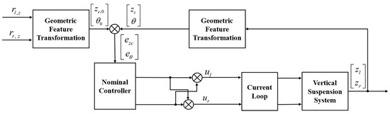
Figure 4. Schematic Diagram of Decoupling Control Based on Geometric Feature Transformation.

Specifically, for the vertical suspension system in Equation (22), the control process is as follows: the setpoint inputs are the target positions of the left and right ends, denoted as $r_{l,z}$ and $r_{r, z}$. First, a predefined geometric transformation module converts the measured position values at the left and right ends into feature quantities representing the overall motion of the magnetically suspension model—namely, the center-of-mass position $z_c$ and the pitch angle $\theta$. Then, a nominal controller receives the deviation signals between the target and measured values of the transformed features $\left(z_c,\theta \right)$. This controller outputs two independent control signals $\left(u_{c,z},u_{c,\theta }\right)$, corresponding to the control requirements for the center-of-mass position and the pitch angle, respectively. Finally, these two control signals are differentially allocated (i.e., $u_l=u_{c,z}+u_{c,\theta }$ and $u_r=u_{c,z}-u_{c,\theta }$), processed through the current loop, and used to drive the corresponding electromagnetic actuators.

The definition of the vertical geometric features of the MSBS is illustrated in Figure 5. The suspension model centroid target position, $z_{c,0}$, is defined as the arithmetic mean of the target positions of the front and rear ends, $z_{l,0}$ and $z_{r,0}$:

$$z_{c,0}={\displaystyle \frac{z_{l,0}+z_{r,0}}{2}}$$

(30)

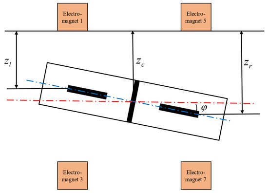
Figure 5. Geometric Features of the Vertical Suspension System.

The target attitude angle ${\theta }_0$ of the system is calculated using the inverse tangent function of the ratio between the difference in the target positions at the two ends and the distance between the suspension points:

$${\theta }_0=\arctan \left({\displaystyle \frac{z_{l,0}-z_{r,0}}{L_{\mathrm{per}}}}\right)$$

(31)

Similarly, the actual position of the center of mass $z_c$ is determined as the arithmetic mean of the actual positions at the left and right ends, $z_l$ and $z_r$:

$$z_c={\displaystyle \frac{z_l+z_r}{2}}$$

(32)

The actual attitude angle of the system is calculated using the inverse tangent function of the ratio between the difference in the actual positions at the two ends and the distance between the suspension points:

$$\theta =\arctan \left({\displaystyle \frac{z_l-z_r}{L_{\mathrm{per}}}}\right)$$

(33)

Based on the above, the geometric coordinate transformation matrix is defined as:

$${\overline{F}}_1=\left[\begin{array}{cc}{\displaystyle \frac{1}{2}}& {\displaystyle \frac{1}{2}}\\ {\displaystyle \frac{1}{L_{\mathrm{per}}}}& -{\displaystyle \frac{1}{L_{\mathrm{per}}}}\end{array}\right]$$

(34)

where ${\overline{F}}_1$ is the geometric coordinate transformation matrix.

PID controller is selected as the nominal controller, and the control law for the center-of-mass geometric feature is:

$$u_{bc}=k_{pc}{e}_{zc}+k_{dc}{\dot{e}}_{zc}+k_{ic}{{\displaystyle \int }}_0^t{e}_{zc}\mathrm{d}t$$

(35)

where $u_{bc}$ is the controller output for center-of-mass, $e_{zc}$ is the error in the center-of-mass geometric feature, and $k_{pc}$, $k_{dc}$ and $k_{ic}$ are the proportional, derivative, and integral gains of the controller for center-of-mass, respectively.

The nominal control law for the attitude angle geometric feature is:

$$u_{b\theta }=k_{p\theta }{e}_{\theta }+k_{d\theta }{\dot{e}}_{\theta }+k_{i\theta }{{\displaystyle \int }}_0^t{e}_{\theta }\mathrm{d}t$$

(36)

where $u_{b\theta }$ is the controller output for attitude angle and $e_{\theta }$ is the error in the attitude angle geometric feature. $k_{d\theta }$ and $k_{i\theta }$ are the proportional, derivative, and integral gains of the controller for attitude angle, respectively.

The expressions for $e_{zc}$ and $e_{\theta }$ are:

$$\left[\begin{array}{c}{e}_{zc}\\ e_{\theta }\end{array}\right]={\overline{F}}_1\left[\begin{array}{c}{z}_l\\ z_r\end{array}\right]-{\overline{F}}_1\left[\begin{array}{c}{r}_{zl}\\ r_{zr}\end{array}\right]$$

(37)

The feedback decoupling strategy based on geometric feature transformation, as developed in this work, deliberately architectures the control system through structural reshaping of the coupled dynamics. This approach fundamentally redefines the interaction mechanisms among control commands. Unlike conventional PID or multivariate control schemes that treat vertical coupling as an external disturbance requiring passive compensation, the proposed method embeds an analytical model of the system coupling directly into the coordinate transformation framework. This enables proactive cancelation of anticipated coupling effects at the control command formulation stage, thereby achieving a paradigm shift from reactive suppression to proactive structural decoupling.

4. Simulation and Experimental Validation

In this section, both experimental studies and simulation results are presented to illustrate the effectiveness of the proposed approach.

4.1. Simulation and Analysis Based on Linear Model

Based on the linearized vertical suspension control system model from Section 2.2 and Section 3.1, simulation verification of the feedback decoupling controller is conducted. First, independent PID controllers are used as the nominal controllers for the front and rear vertical attitude control:

$$K_{\mathrm{vn},11}=k_{P_1}+k_{I_1}{\displaystyle \frac{1}{s}}+k_{D_1}{\displaystyle \frac{k_{N_1}}{1+k_{N_1}\frac{1}{s}}}$$

(38)

$$K_{\mathrm{vn},22}=k_{P_2}+k_{I_2}{\displaystyle \frac{1}{s}}+k_{D_2}{\displaystyle \frac{k_{N_2}}{1+k_{N_2}\frac{1}{s}}}$$

(39)

where $k_{P_1}$, $k_{I_1}$, $k_{D_1}$ and $k_{N_1}$ are the proportional, integral, derivative, and filter coefficients for the left controller $K_{\mathrm{vn},11}$. $k_{P_2}$, $k_{I_2}$, $k_{D_2}$, $k_{N_2}$ are the corresponding coefficients for the right controller $K_{\mathrm{vn},22}$.

The PID controller parameters are set as $k_{P_1}=k_{P_2}=17$, $k_{I_1}=k_{I_2}=53$, $k_{D_1}=k_{D_2}=0.95$, $k_{N_1}=k_{N_2}=373$. Figure 6 shows the curves of the front vertical position $x_1$ and rear vertical position $x_4$ of the magnetically suspension model without decoupling. Both the front and rear ends exhibit oscillations with an amplitude of approximately 0.002 m. A magnified view clearly reveals that the displacement curves at both ends exhibit nearly sinusoidal fluctuations with a period of about 0.005 s (corresponding to a frequency of 200 Hz) and a phase difference of 180°. This further confirms the presence of significant dynamic coupling between the front and rear vertical degrees of freedom in the MSBS. When independent control is applied to the electromagnets at both ends, the front and rear ends show periodic vibrations with equal amplitude and opposite phase (180° phase difference), indicating that the vertical suspension system exhibits a typical pitch vibration mode without decoupling. This mode oscillates persistently at a natural frequency of about 200 Hz, causing disturbances on one side to trigger cooperative oscillations on both sides. This phenomenon profoundly reveals the strong coupling between the mechanical structural dynamics and the control loops. Therefore, a decoupling controller must be designed to suppress this inherent vibrational mode and improve the stability of the vertical suspension system.

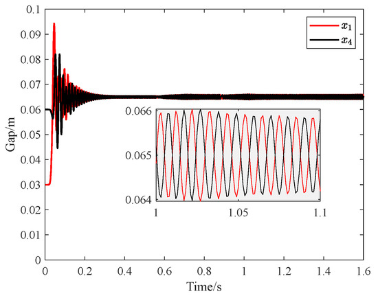
Figure 6. Vertical Positions of the Front and Rear Ends Without Decoupling.

Combining the parameters of the vertical electromagnet array and the magnetically suspension model, the expressions for the state feedback matrix ${\overline{K}}_{\mathrm{v}}$ and input transformation matrix ${\overline{F}}_{\mathrm{v}}$ are obtained as:

$$\left\{\begin{array}{l}{\overline{K}}_{\mathrm{v}}=\left[\begin{array}{cccccc}0& -0.0179& 0.23& 0& 0.0118& 0\\ 0& 0.0118& 0& 0& -0.0179& 0.23\end{array}\right]\\ {\overline{F}}_{\mathrm{v}}=\left[\begin{array}{cc}1.0393\times {10}^{-4}& -2.5362\times {10}^{-5}\\ -2.5362\times {10}^{-5}& 1.0393\times {10}^{-4}\end{array}\right]\end{array}\right.$$

(40)

For the decoupled system, controllers $K_{\mathrm{vn},11}$ and $K_{\mathrm{vn},22}$ are still used as nominal controllers. Figure 7 shows a comparison of the front and rear vertical position responses of the model under the decoupling control strategy and the nominal control strategy. Both control laws enable stable convergence from the initial position to the target setpoint. Notably, compared to the independent nominal controller, the designed decoupling controller demonstrates performance improvements. The displacement response curves at both ends show no trace of the previously observed coupling-induced anti-phase sinusoidal oscillations. The steady-state error is minimal, and the settling time is significantly reduced, indicating excellent dynamic performance and steady-state accuracy under decoupling control. Detailed comparative results are summarized in Table 2 and Table 3. These results strongly validate the effectiveness of the decoupling control strategy in suppressing the vertical-pitch coupled dynamic modes and enhancing the overall stability of the closed-loop system.

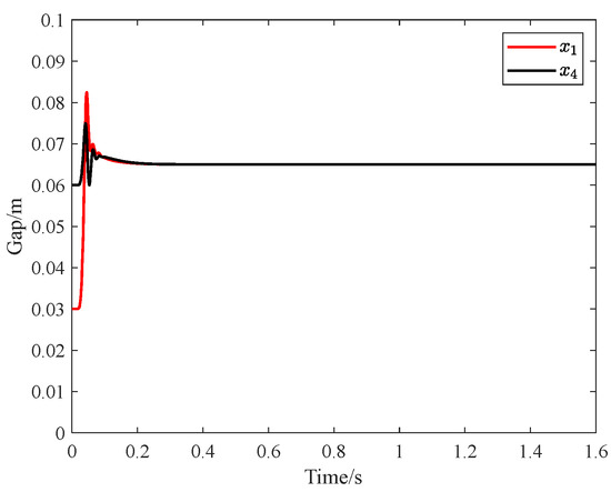
Figure 7. Control Performance Based on Feedback Decoupling.

Table 2. Detailed comparative results of $x_1$.

Indicator	Steady-State Error	Peak Value	Vibration Frequency
Without Decoupling	0.001033	0.0943	200 Hz
Feedback Decoupling	0	0.0824	0 Hz

Table 3. Detailed comparative results of $x_4$.

Indicator	Steady-State Error	Peak Value	Vibration Frequency
Without Decoupling	0.001016	0.0820	200 Hz
Feedback Decoupling	0	0.0749	0 Hz

4.2. Simulation and Analysis Based on Nonlinear Model

From Section 3.2, the design of the feedback decoupling controller relies on the linearized system model. However, the actual vertical suspension system of the MSBS exhibits unmodeled nonlinear dynamics and parameter uncertainties, leading to significant degradation of the theoretical decoupling performance in practical closed-loop control. To verify its robustness, the designed feedback decoupling controller is applied to a nonlinear system model for testing, yielding the position curves shown in Figure 8. The simulation results show that although the controller achieves stable tracking of the target setpoint, the response curves exhibit sustained low-amplitude oscillations, and the front and rear vertical displacements show asymmetric fluctuation characteristics. Therefore, under strongly nonlinear conditions, the feedback decoupling mechanism based on ideal linear assumptions cannot fully eliminate the inherent vertical-pitch coupling mode, and its decoupling effectiveness is significantly reduced due to model mismatch.

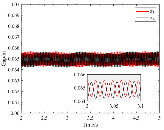
Figure 8. The impact of model nonlinearity on decoupling controller.

To verify the performance of the geometric feature transformation-based decoupling controller under nonlinear conditions, the simulation directly used the full-order nonlinear magnetic suspension model as the controlled plant (i.e., without linear approximation). The controller parameters in Equations (35) and (36) are set as $k_{pc}=290$, $k_{dc}=25$, $k_{ic}=20$, $k_{p\theta }=22$, $k_{d\theta }=2$, $k_{i\theta }=1.5$. Figure 9 shows a comparison of the results under two control strategies. Under the independent control strategy, the pitch attitude angle exhibits sustained constant-amplitude oscillations with a steady-state amplitude of 1.8°, indicating that the pitch-vertical coupling mode of the un-decoupled system is not effectively suppressed. In contrast, under the geometric feature transformation-based decoupling controller, the pitch angle rapidly converges from an initial offset of 0.57° to the target value of 0° without overshoot or oscillation. The response curve shows strictly monotonic convergence characteristics throughout both the transient adjustment and steady-state phases. Thus, the proposed decoupling controller overcomes the stability limitations of traditional independent control and achieves dynamic decoupling of the vertical/pitch channels in a strongly nonlinear system.

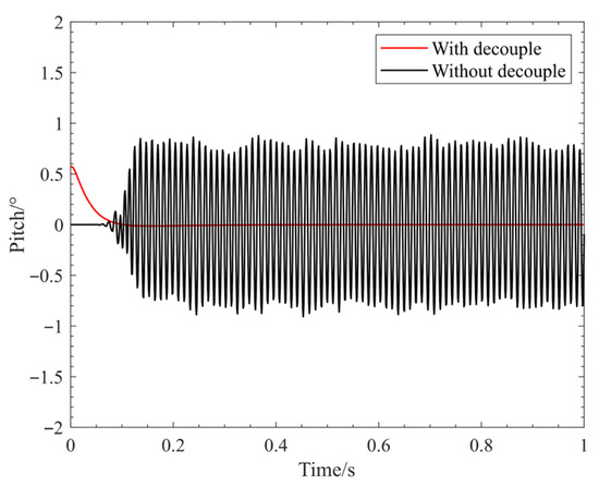
Figure 9. Attitude Angle Under Geometric Feature Transformation-Based Decoupling Control.

Figure 10 shows the vertical displacements of the left/right endpoints and the center-of-mass vertical displacement of the model under geometric feature transformation-based decoupling control. The results indicate that all three curves converge to the target position with small steady-state errors. The transient trajectories of the three positions change in strict synchrony, and no significant oscillations occur in the steady-state phase. The vertical-pitch coupled vibrations are completely suppressed.

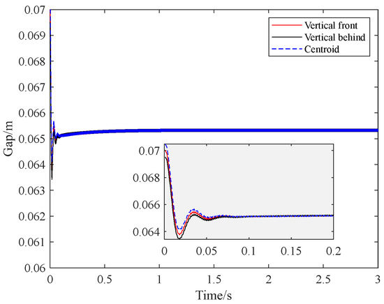
Figure 10. Vertical Position Curves Under Geometric Feature Transformation-Based Decoupling Control.

4.3. Experimental Validation and Analysis

This section verifies the effectiveness of the proposed estimation method using suspension data from the axial suspension system of a MSBS, as shown in Figure 11, developed by the College of Intelligence Science and Technology, National University of Defense Technology. Through an H-type linear CCD attitude detection system and current sensors, real-time acquisition of the suspension model’s positional data and current signals is performed. This data is transmitted to the controller for computation. The controller outputs PWM signals to the silicon carbide (SiC) chopper, actuating the power supply to energize the electromagnets. The resulting electromagnetic force counteracts the gravitational and aerodynamic loads on the model.

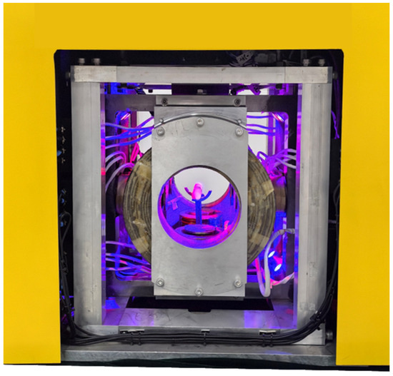
Figure 11. Physical Setup of the Wind Tunnel MSBS.

Vertical suspension control experiments were conducted on a dedicated MSBS experimental test platform. The sampling time of the vertical suspension control system is set to 0.5 ms. Independent PID controllers are used to control the front and rear ends of the experimental model, with controller parameters set as $k_{P_1}=k_{P_2}=1$, $k_{I_1}=k_{I_2}=0.15$, $k_{D_1}=k_{D_2}=0.05$, $k_{N_1}=k_{N_2}=800$. Figure 12 shows the vertical position curves of the front and rear ends of the magnetically suspension model without decoupling. As illustrated, the displacement curves of both the front and rear ends exhibit periodic fluctuations. The fluctuation amplitude of the front end is 0.006 m, which is larger than that of the rear end which is 0.005 m.

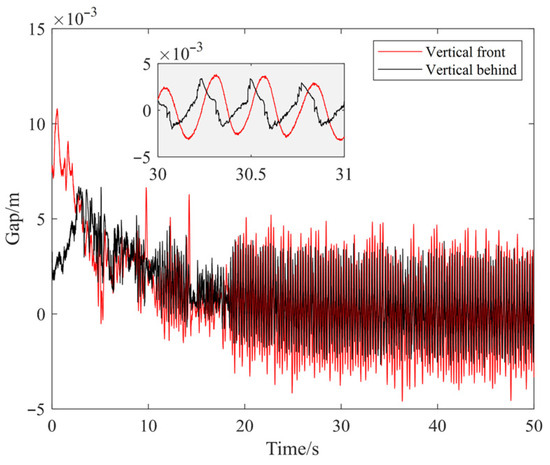
Figure 12. Vertical Position Without Decoupling.

From the zoomed-in section between 30 s and 31 s, it can be clearly observed that both exhibit a vibration pattern approximating a sinusoidal waveform, with a vibration period of approximately 0.015 s, corresponding to a frequency of about 66.7 Hz. Furthermore, the phase difference between the vibrations of the front and rear ends is close to 180°, meaning they move in opposite directions, demonstrating a clear anti-phase oscillation mode. This anti-phase vibration is a typical manifestation of vertical coupling, indicating strong dynamic coupling effects within the system. Therefore, the vertical suspension system of the MSBS exhibits significant coupled vibration, with the front and rear ends demonstrating anti-phase sinusoidal oscillation, necessitating effective decoupling strategies.

Figure 13 shows the vertical position of the suspension model under the geometric feature transformation-based decoupling controller. The vertical motion characteristics of the MSBS are significantly improved under this controller. After 10 s, the vertical position of the model rapidly reaches a stable state, with the steady-state error maintained within a small range. Specifically, the fluctuation amplitude of the front end ranged from −1 mm to 1.5 mm, while that of the rear end ranged from −0.5 mm to 0.5 mm. The displacement curves of the front and rear ends show highly consistent and synchronous variation characteristics during both transient and steady-state phases, with no significant phase difference or anti-phase oscillation observed between their trajectories. This result clearly indicates that the original vertical-pitch coupled vibration has been effectively suppressed, further demonstrating that the controller not only possesses excellent decoupling capability but also ensures system stability and dynamic response performance. Consequently, these experimental results fully validate the effectiveness of the geometric feature transformation-based decoupling control strategy for the magnetic suspension system, providing a reliable experimental basis for the decoupling control of complex multi-degree-of-freedom systems like the MSBS.

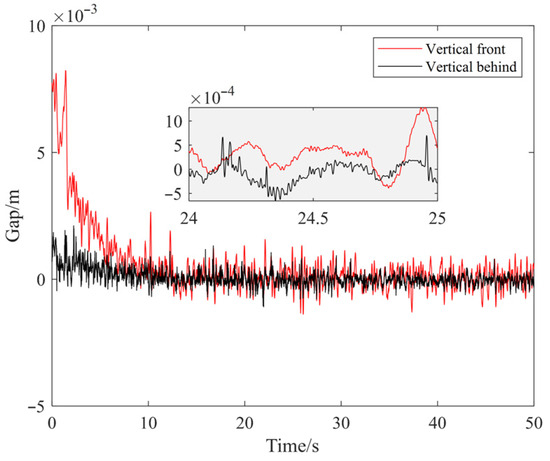
Figure 13. Vertical Position Under Geometric Feature Transformation-based Decoupling Controller.

5. Conclusions

This study addresses the strong mechanical coupling in the vertical suspension system of a supersonic wind tunnel magnetic suspension balance by establishing a six-degree-of-freedom nonlinear dynamic model. Through linearization analysis of the vertical subsystem, the coupling mechanism between rigid body translation and rotation induced by the off-diagonal terms in the state equation is revealed. Simulations and experiments demonstrate that this coupling excites a high-frequency pitch oscillation at 200 Hz in the linearized model, with a simulated amplitude of 0.002 m, while manifesting as a low-frequency beat vibration at 66.7 Hz in the actual nonlinear system, with an experimental amplitude of 0.006 m. Such an anti-phase vibration mode leads to unsatisfactory performance of independent control strategies and makes the system prone to instability.

Based on above analysis, a state feedback decoupling control method is investigated, which completely suppresses the oscillation in the ideal linear model, achieving smooth, overshoot-free stable convergence. However, its performance heavily depends on model parameters, resulting in limited decoupling effectiveness in the practical system. Subsequently, a geometric feature transformation-based decoupling controller is proposed. Simulations with the full-order nonlinear model demonstrate oscillation-free convergence of the pitch angle from 0.57° to 0°, and experiments confirm its efficacy in suppressing the 66.7 Hz vibration, significantly reducing vertical displacement fluctuations. This method successfully eliminates the vertical-pitch coupled mode, enabling the system to stabilize within 10 s. By reconstructing the state space, it overcomes the limitations of traditional methods under nonlinear conditions, providing a more robust control framework for the MSBS and enhancing the reliability of aerodynamic testing.

References

- Liu, Y.; Wang, Y.; Yuan, C.; Luo, C.; Jiang, Z. Aerodynamic force and moment measurement of 10° half-angle cone in JF12 shock tunnel. Chin. J. Aeronaut. 2017, 30, 983–987. [Google Scholar] [CrossRef]
- Oshima, R.; Sawada, H.; Obayashi, S. A development of dynamic wind tunnel test technique by using a magnetic suspension and balance system. In Proceedings of the American Institute of Aeronautics and Astronautics Inc, AIAA, San Diego, CA, USA, 4–8 January 2016; pp. 1541–1555. [Google Scholar]
- Park, K.; Sung, Y.; Han, J. Cable suspension and balance system with low support interference and vibration for effective wind tunnel tests. Int. J. Aeronaut. Space Sci. 2021, 22, 1048–1061. [Google Scholar] [CrossRef]
- Kai, D.; Sugiura, H.; Tezuka, A. Magnetic suspension and balance system for high-subsonic wind tunnel. AIAA J. 2019, 57, 2489–2495. [Google Scholar] [CrossRef]
- Lee, D.K.; Lee, J.S.; Han, J.H.; Kawamura, Y. Dynamic calibration of magnetic suspension and balance system for sting-free measurement in wind tunnel tests. J. Mech. Sci. Technol. 2013, 27, 1963–1970. [Google Scholar] [CrossRef]
- Kobayashi, T.; Seo, K.; Kaneda, S.; Sasaki, K.; Shinji, K.; Oyama, S.; Okuizumi, H.; Konishi, Y.; Hasegawa, H.; Obayashi, S. Measurement of the aerodynamic forces acting on a non-spinning javelin using an MSBS. Proceedings 2020, 49, 144–152. [Google Scholar] [CrossRef]
- Shehata, H.; Cox, D.; Schoenenberger, M.; Britcher, C.P.; Shellabarger, E.; Schott, T.; McGovern, B. The Feasibility of Motion Tracking Camera System for Magnetic Suspension Wind Tunnel Tests. In Proceedings of the AIAA SCITECH 2024 Forum, Orlando, FL, USA, 8–12 January 2024; p. 1918. [Google Scholar]
- Tashiro, K.; Yokota, S.; Zigunov, F.; Ozawa, Y.; Asai, K.; Nonomura, T. Slanted cylinder afterbody aerodynamics measured by 0.3-m magnetic suspension and balance system with six-degrees-of-freedom control. Exp. Fluids 2022, 63, 119. [Google Scholar] [CrossRef]
- Senda, H.; Sawada, H.; Okuizumi, H.; Konishi, Y.; Obayashi, S. Aerodynamic measurements of AGARD-B model at high angles of attack by 1-m magnetic suspension and balance system. In Proceedings of the 2018 AIAA Aerospace Sciences Meeting, Kissimmee, FL, USA, 8–12 January 2018; p. 0302. [Google Scholar]
- Xia, W.; Dou, F.; Long, Z. A disturbance force compensation framework for a magnetic suspension balance system. Actuators 2023, 12, 98. [Google Scholar] [CrossRef]
- Lee, D.K.; Lee, J.S.; Han, J.H.; Kawamura, Y.; Chung, S.J. Development of a simulator of a magnetic suspension and balance system. Int. J. Aeronaut. Space Sci. 2010, 11, 175–183. [Google Scholar] [CrossRef]
- Neill, C.K. Comparison of Support Methods for Static Aerodynamic Testing and Validation of a Magnetic Suspension and Balance System. Master’s Thesis, Old Dominion University, Norfolk, VA, USA, 2019. [Google Scholar]
- Lee, D. Design of robust control system of magnetic suspension and balance system through harmonic excitation simulation. Aerospace 2021, 8, 304–318. [Google Scholar] [CrossRef]
- Sawada, H.; Umezawa, K.; Yokozeki, T.; Watanabe, A. Wind tunnel test of Japanese arrows with the JAXA 60-cm magnetic suspension and balance system. Exp. Fluids. 2012, 53, 451–466. [Google Scholar] [CrossRef]
- Kai, D.; Sugiura, H.; Tezuka, A. Development of magnetic suspension and balance system for high-subsonic wind tunnel. In Proceedings of the 2018 AIAA Aerospace Sciences Meeting, Kissimmee, FL, USA, 8–12 January 2018; pp. 304–317. [Google Scholar]
- Takagi, Y.; Sawada, H.; Obayashi, S. Development of magnetic suspension and balance system for intermittent supersonic wind tunnels. AIAA J. 2016, 54, 1277–1286. [Google Scholar] [CrossRef]
- Wang, H.; Liu, G.; Yin, L.M. Discrete Sliding mode variable structure control of MSBS. Control. Theory Appl. 2004, 23, 13–14. [Google Scholar]
- Xia, W.; Long, Z.; Dou, F. System modeling and control system performance optimization of magnetic suspension and balance system. Int. J. Appl. Electromagn. Mech. 2022, 68, 105–122. [Google Scholar] [CrossRef]
- Britcher, C.; McGovern, B.; Cox, D.; Schoenenberger, M. An investigation of bluff body corrections using the NASA/ODU 6-inch MSBS. In Proceedings of the 19th International Conference on Flow Dynamics (ICFD2022), Sendai, Japan, 9–11 November 2022. [Google Scholar]
- Britcher, C.P.; Cox, D.E. Electromagnetic modeling of wind tunnel magnetic suspension and balance systems. In Proceedings of the AIAA SCITECH 2023 Forum, National Harbor, MD, USA, 23–27 January 2023; p. 1819. [Google Scholar]
- Schoenenberger, M.; Cox, D.; Britcher, C. Forced Displacement Technique for Measuring Blunt Body Aerodynamics in a Magnetic Suspension Wind Tunnel. In Proceedings of the 21st International Conference on Flow Dynamics (ICFD), Sendai, Japan, 18–20 November 2024. [Google Scholar]
- Zhao, Z.; Xu, Y.; Wen, G. Gradient-based performance optimization for flight control system with real-time data. IEEE Trans. Syst. Man Cybern. Syst. 2025, 55, 2537–2545. [Google Scholar] [CrossRef]
- Shinji, K.; Nagaike, H.; Nonomura, T.; Asai, K.; Okuizumi, H.; Konishi, Y.; Sawada, H. Aerodynamic characteristics of low-fineness-ratio freestream-aligned cylinders with magnetic suspension and balance system. AIAA J. 2020, 58, 3711–3714. [Google Scholar] [CrossRef]
- Sung, Y.H.; Lee, D.K.; Han, J.S.; Kim, H.Y.; Han, J.H. MSBS-SPR integrated system allowing wider controllable range for effective wind tunnel test. Int. J. Aeronaut. Space Sci. 2017, 18, 414–424. [Google Scholar] [CrossRef]
- Nonomura, T.; Sato, K.; Fukata, K.; Nagaike, H.; Okuizumi, H.; Konishi, Y.; Asai, K.; Sawada, H. Effect of fineness ratios of 0.75–2.0 on aerodynamic drag of freestream-aligned circular cylinders measured using a magnetic suspension and balance system. Exp. Fluids 2018, 59, 77. [Google Scholar] [CrossRef]
- Guo, S.; Bai, C. Coupling effect of unbalanced magnetic pull and ball bearing on nonlinear vibration of motor rotor system. J. Vib. Control 2022, 28, 665–676. [Google Scholar] [CrossRef]
- Xia, W.; Zeng, J.; Dou, F.; Long, Z. Method of combining theoretical calculation with numerical simulation for analyzing effects of parameters on the maglev vehicle-bridge system. IEEE Trans. Veh. Technol. 2021, 70, 2250–2257. [Google Scholar] [CrossRef]
- Pan, C.; Wang, C.; Liu, Z.; Chen, X. Winding vibration analysis of unbalanced transformer based on electromagnetic-mechanical coupling. Int. J. Electr. Power Energy Syst. 2022, 134, 107459. [Google Scholar] [CrossRef]
- Zou, Y.; Zhu, J.; Liu, Y. State-feedback controller design for disturbance decoupling of Boolean control networks. IET Control Theory Appl. 2017, 11, 3233–3239. [Google Scholar] [CrossRef]
- Yin, Z.; Cai, Y.; Ren, Y.; Wang, W.; Chen, X.; Yu, C. Decoupled active disturbance rejection control method for magnetically suspended rotor based on state feedback. J. Beijing Univ. Aeronaut. Astronaut. 2021, 48, 1210–1221. [Google Scholar]
- Xu, Y.; Zhao, Z.; Yin, S.; Long, Z. Real-time performance optimization of electromagnetic levitation systems and the experimental validation. IEEE Trans. Ind. Electron. 2022, 70, 3035–3044. [Google Scholar] [CrossRef]
- Xu, Y.; Zhao, Z.; Yin, S. Performance optimization and fault-tolerance of highly dynamic systems via Q-learning with an incrementally attached controller gain system. IEEE Trans. Neural Netw. Learn. Syst. 2022, 34, 9128–9138. [Google Scholar] [CrossRef] [PubMed]
Disclaimer/Publisher’s Note: The statements, opinions and data contained in all publications are solely those of the individual author(s) and contributor(s) and not of MDPI and/or the editor(s). MDPI and/or the editor(s) disclaim responsibility for any injury to people or property resulting from any ideas, methods, instructions or products referred to in the content. |
© 2025 by the authors. Licensee MDPI, Basel, Switzerland. This article is an open access article distributed under the terms and conditions of the Creative Commons Attribution (CC BY) license (https://creativecommons.org/licenses/by/4.0/).