Research on Additive Manufacturing Path Planning of a Six-Degree-of-Freedom Manipulator

Abstract

The research on additive manufacturing (AM) path planning mainly focuses on the traditional three-axis AM path planning and five-degree-of-freedom (DOF) AM path planning, while there is less research on six-DOF AM path planning. In the traditional AM path planning algorithm, the filling path is discontinuous and there is long straight-line printing in a certain direction, which can easily lead to warpage deformation. Therefore, in this work, the six-DOF manipulator is taken as the main object to build an AM platform, and the mechanism of AM path planning of the manipulator is studied. The path planning algorithm combining the contour offset filling method and Hilbert curve filling is optimized by using a cubic uniform B-spline curve, and an AM path planning algorithm suitable for a six-DOF manipulator is obtained. A continuous printing path can be generated by this algorithm. It reduces the existence of long straight-line printing in a certain direction, thereby reducing the warpage deformation of the model and improving the molding quality of the model. The traditional three-axis AM device and the six-DOF AM platform were used to print two kinds of models. By comparing the printing time, the six-DOF AM platform was 43.70% and 37.94% shorter than the traditional three-axis AM device. The same model was printed on a six-DOF AM platform by using the parallel scanning filling method, the path planning algorithm combining contour offset and Hilbert curve, and the method proposed in this paper. Through experimental verification, the average warpage deformation of the model printed by the method proposed in this paper was reduced by 37.81% and 13.79%, respectively, compared with the other two methods.

1. Introduction

Additive manufacturing (AM), also known as 3D printing, is a kind of rapid prototyping technology. Because of its advantages of fast forming speed, high processing precision, and high material utilization rate, it has broad application prospects [1]. It has been applied in industrial production [2,3], biomedical [4], aerospace [5], emerging education [6], emerging consumption, and so on.

Commonly used path planning algorithms mainly include the parallel scanning filling method, contour offset filling method, and spatial curve filling method. As an important part of AM research, path planning has been studied by many scholars. In the aspect of traditional AM path planning, Jin et al. [7] proposed a parallel scanning path planning optimization algorithm for fused deposition modeling. By selecting the optimal scanning line angle and studying the relationship between the scanning line angle and the printing efficiency and surface quality, an adaptive region merging algorithm is developed. Yang et al. [8] proposed a contour offset path generation algorithm, which provides an efficient solution for path planning. However, because of the large curvature of the contour offset path, the frequent bending path makes the motor accelerate and decelerate frequently, so the printing efficiency is low. Aiming at the problem that the spiral offset path planning algorithm has difficulty dealing with the continuous filling path of different sub-regions, Yu et al. [9] proposed a global continuous Fermat spiral path planning algorithm for carbon fiber 3D printing, but the algorithm has poor filling effect in the case of sharp corners in the filling path. Yang and Mohan et al. [10,11] proposed a path filling method of the Hilbert space curve, which can improve the printing efficiency of the model. However, because of the existence of multiple right-angle corners in the Hilbert curve, the motor starts and stops more frequently.

In multi-DOF AM path planning, Zhao et al. [12] proposed a hybrid path planning method based on skeleton contour division, which reduces the sharp corners in the contour and the impact on the forming quality. Dong et al. [13] proposed a contour path planning algorithm for optimizing deposition additive manufacturing. The Hopfield neural network and the improved whale optimization algorithm are used to sort the printing order of each contour and optimize the network parameters. Diourté et al. [14] proposed a five-DOF continuous path planning algorithm, which can realize continuous printing paths for closed-loop spiral parts. Isa [15] proposed a five-axis path planning method for FDM. The algorithm can effectively eliminate the staircase effect. Guacheta-Alba J C et al. [16] proposed a six-DOF path planning algorithm based on contour parallel mode, which can generate continuous printing paths. Nguyen et al. [17] proposed an automatic tool path planning method based on offset contour. The generated toolpath is a globally continuous, layer-wise setting, making it suitable for robotic cold spray additive manufacturing.

At present, the research on AM path planning mainly focuses on traditional three-axis AM path planning and five-DOF AM path planning. There are relatively few studies on six-DOF AM path planning, but it is very important to realize efficient printing of parts. In most traditional AM path planning algorithms, the printing path is discontinuous and there is long straight-line printing in a certain direction. For traditional AM devices, a discontinuous printing path represents an increase in the number of motors starts and stops, resulting in a longer printing time. For multi-DOF AM, a discontinuous printing path will lead to an increase in the number of start–stop times of the motor of the consumables conveying mechanism, and it is impossible to maintain a stable wire-feeding state. The main reason for warpage deformation is the thermal expansion and contraction of the material and the residual stress caused by the temperature change. This phenomenon is particularly serious when there is long straight-line printing in a certain direction.

In view of the above problems, in this paper, a six-DOF manipulator is taken as the research object, an AM platform is built, and related experiments are carried out. The path planning algorithm combining the contour offset filling method and Hilbert curve filling is optimized by using a cubic uniform B-spline, and an AM path planning algorithm suitable for a six-DOF manipulator is obtained.

(1) Based on the homogeneous transformation matrix and the modified D-H method, the mechanism of path planning of the six-DOF manipulator is studied, including kinematics modeling, forward and inverse kinematics analysis of the manipulator, and the simulation of motion space and printing path.

(2) The models are printed on the traditional three-axis AM device and the six-DOF AM platform by using parallel scanning filling methods. By comparing the printing time, it is verified that the six-DOF AM platform has higher printing efficiency.

(3) The parallel scanning filling method, the path planning algorithm combining contour offset and Hilbert curve, and the method proposed in this paper are used to print the model, and the warping deformation of the model is compared to prove the effectiveness and practicability of the proposed method.

2. Kinematics Analysis Based on the Homogeneous Transformation Matrix and Modified D-H Method

2.1. Motion Principle of Mechanical Arm

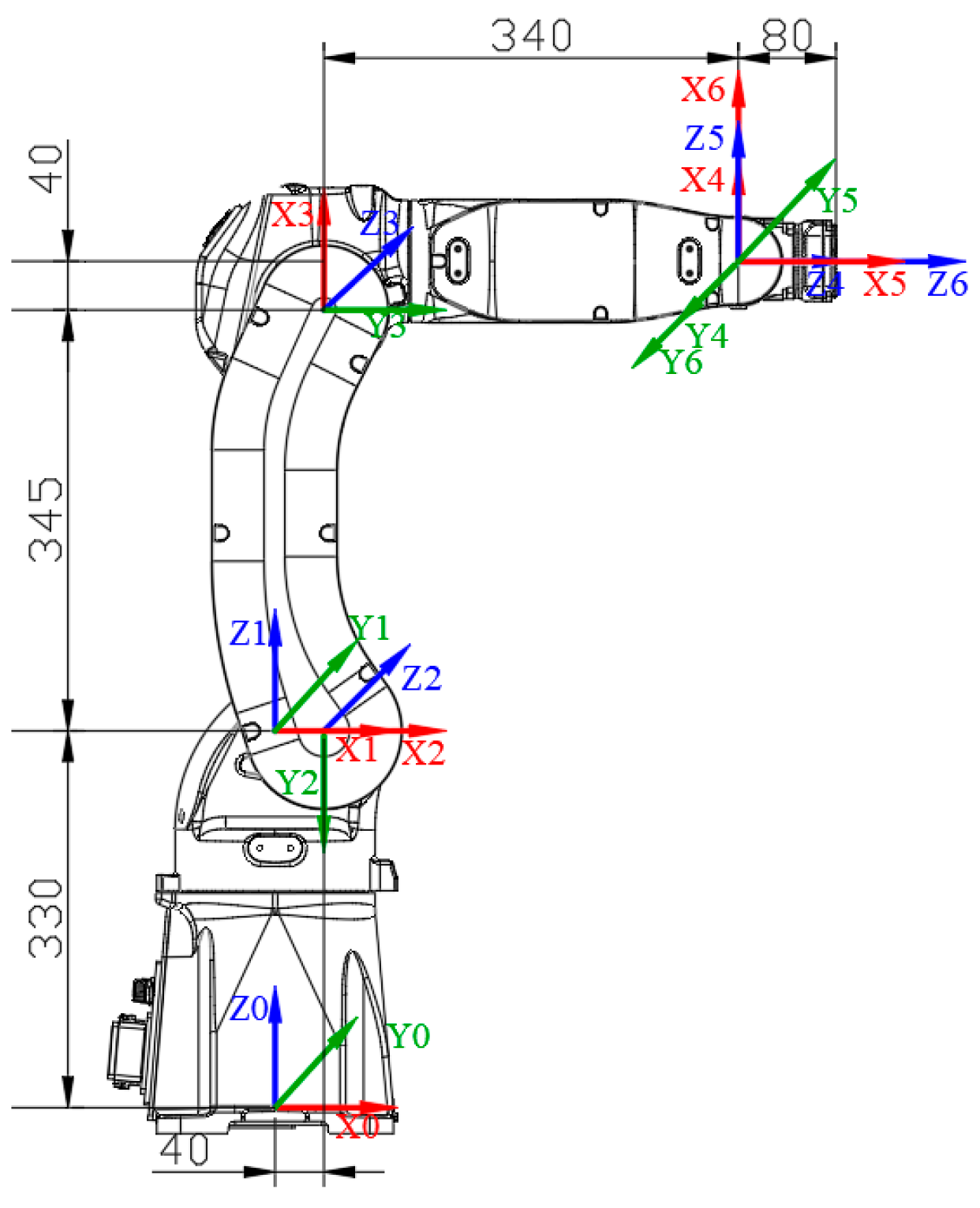
The six-DOF manipulator used in this paper is the Yaskawa GP8 manipulator, and its six kinematic pairs are all rotating joints. The first three joints of the GP8 manipulator determine the position of the wrist reference point, and the last three joints determine the direction of the wrist, which belongs to the 6R manipulator. The body structure and joint coordinate system are shown in Figure 1.

Figure 1. The body structure and joint coordinate system of GP8 manipulator.

Commonly used manipulator motion modeling methods mainly include the standard D-H method and the modified D-H method [18]. According to the joint coordinates of the manipulator, the modified DH method is used to model the motion of the manipulator. The D-H parameters are shown in Table 1:

Table 1. D-H parameter table of the GP8 manipulator.

Link (i)	Connecting Rod Offset ${\mathit{d}}_{\mathit{i}}/\mathbf{mm}$	Connecting Rod Length ${\mathit{a}}_{\mathit{i}-1}/\mathbf{mm}$	Connecting Rod Torsion Angle ${\mathit{\alpha }}_{\mathit{i}-1}/°$	Joint Rotation Angle ${\mathit{\theta }}_{\mathit{i}}/°$	Offset $/°$
1	D1	0	0	θ1	0
2	0	L2	−90	θ2	−90
3	0	L3	0	θ3	0
4	D4	L4	−90	θ4	0
5	0	0	−90	θ5	0
6	0	0	90	θ6	±180

The offset term in the above table is the angle between the drive shaft and the transmission shaft when the robot is at zero, where D₁ = 330, L₂ = 40, L₃ = 345, L₄ = 40, and D₄ = 340.

2.2. Forward Kinematics Analysis and Inverse Kinematics Analysis of the Manipulator

The forward kinematics of the manipulator describes that the joint angle ${\theta }_i$ of each joint in the joint space of the manipulator is known, and the pose of the end effector of the manipulator in the Cartesian coordinate system is obtained. According to the law of translation and rotation [18], the following conversion relationship between the two adjacent coordinate systems can be obtained.

$${}_i{}^{i-1}T=\left[\begin{array}{cccc}c{\theta }_i& -s{\theta }_i& 0& a_{i-1}\\ s{\theta }_{i}c{\alpha }_{i-1}& c{\theta }_{i}c{\alpha }_{i-1}& -s{\alpha }_{i-1}& -s{\alpha }_{i-1}{d}_i\\ s{\theta }_{i}s{\alpha }_{i-1}& c{\theta }_{i}s{\alpha }_{i-1}& c{\alpha }_{i-1}& c{\alpha }_{i-1}{d}_i\\ 0& 0& 0& 1\end{array}\right]$$

(1)

where $c{\theta }_i=\cos {\theta }_i$ and $s{\theta }_i=\sin {\theta }_i$. According to the established D-H parameter table, the homogeneous transformation matrix ${}_i{}^{i-1}T(i=1,2,\cdots ,6)$ of each joint coordinate system can be obtained. Substituting the parameters of the manipulator in Table 1 into Formula (1), the homogeneous transformation matrix of each joint can be obtained.

$${}_1{}^{0}T=\left[\begin{array}{cccc}c{\theta }_1& -s{\theta }_1& 0& 0\\ s{\theta }_1& c{\theta }_1& 0& 0\\ 0& 0& 1& D_1\\ 0& 0& 0& 1\end{array}\right]$$

(2)

$${}_2{}^{1}T=\left[\begin{array}{cccc}c{\theta }_2& -s{\theta }_2& 0& L_2\\ 0& 0& 1& 0\\ -s{\theta }_2& -c{\theta }_2& 0& 0\\ 0& 0& 0& 1\end{array}\right]$$

(3)

$${}_3{}^{2}T=\left[\begin{array}{cccc}c{\theta }_3& -s{\theta }_3& 0& L_3\\ s{\theta }_3& c{\theta }_3& 0& 0\\ 0& 0& 1& 0\\ 0& 0& 0& 1\end{array}\right]$$

(4)

$${}_4{}^{3}T=\left[\begin{array}{cccc}c{\theta }_4& -s{\theta }_4& 0& L_4\\ 0& 0& 1& D_4\\ -s{\theta }_4& -c{\theta }_4& 0& 0\\ 0& 0& 0& 1\end{array}\right]$$

(5)

$${}_5{}^{4}T=\left[\begin{array}{cccc}c{\theta }_5& -s{\theta }_5& 0& 0\\ 0& 0& 1& 0\\ -s{\theta }_5& -c{\theta }_5& 0& 0\\ 0& 0& 0& 1\end{array}\right]$$

(6)

$${}_6{}^{5}T=\left[\begin{array}{cccc}c{\theta }_6& -s{\theta }_6& 0& 0\\ 0& 0& -1& 0\\ s{\theta }_6& c{\theta }_6& 0& 0\\ 0& 0& 0& 1\end{array}\right]$$

(7)

The expression of the homogeneous transformation matrix ${}_6{}^{0}T$ of the end effector relative to the base coordinate system is as follows:

$${}_6{}^{0}T={\displaystyle {\prod _{i=1}^6}_i^{i-1}}T({\theta }_i)$$

(8)

An expansion of Formula (8) can be obtained.

$${}_6{}^{0}T{=}_1^0{T}_2^1{T}_3^2{T}_4^3{T}_5^4{T}_6^{5}T=\left[\begin{array}{cccc}{r}_{11}& r_{12}& r_{13}& p_x\\ r_{21}& r_{22}& r_{23}& p_y\\ r_{31}& r_{32}& r_{33}& p_z\\ 0& 0& 0& 1\end{array}\right]$$

(9)

The meaning of each element in the matrix is as follows, where $c_{23}=c_2{c}_3-s_2{s}_3$ and $s_{23}=c_2{s}_3+s_2{c}_3$.

$$\begin{array}{l}{r}_{11}=s_6(c_4{s}_1-s_4{c}_1{c}_{23})+c_6[s_5{c}_1{s}_{23}+c_5(s_1{s}_4+c_4{c}_1{c}_{23})]\\ r_{12}=c_6(c_4{s}_1-s_4{c}_1{c}_{23})-s_6[s_5{c}_1{s}_{23}+c_5(s_1{s}_4+c_4{c}_1{c}_{23})]\\ r_{13}=-c_5{c}_1{s}_{23}+s_5(s_1{s}_4+c_4{c}_1{c}_{23})\\ r_{21}=c_6[s_5{s}_1{s}_{23}-c_5(c_1{s}_4-c_4{s}_1{c}_{23})]-s_6(c_1{c}_4+s_4{s}_1{c}_{23})\\ r_{22}=-s_6[s_5{s}_1{s}_{23}-c_5(c_1{s}_4-c_4{s}_1{c}_{23})]-c_6(c_1{c}_4+s_4{s}_1{c}_{23})\\ r_{23}=-s_5(c_1{s}_4-c_4{s}_1{c}_{23})-c_5{s}_1{s}_{23}\\ r_{31}=s_4{s}_6{s}_{23}+c_6(s_5{c}_{23}-c_4{c}_5{s}_{23})\\ r_{32}=c_6{s}_4{s}_{23}-s_6(s_5{c}_{23}-c_4{c}_5{s}_{23})\\ r_{33}=-c_4{c}_5{s}_{23}-c_5{c}_{23}\\ p_x=L_2{c}_1-D_4{c}_1{s}_{23}+L_4{c}_1{c}_{23}+L_3{c}_1{c}_2\\ p_y=L_2{s}_1-D_4{s}_1{s}_{23}+L_3{c}_2{s}_1+L_4{s}_1{c}_{23}\\ p_z=D_1-L_3{s}_2-D_4{c}_{23}-L_3{s}_{23}\end{array}$$

The inverse kinematics of the manipulator describes the joint angle ${\theta }_i$ of each joint in the manipulator when the parameters of each joint and connecting rod of the manipulator and the relative pose relationship between the end effector and the base coordinate system are determined. At present, the methods for solving inverse kinematics mainly include the analytical method and the numerical method [18].

2.3. Mechanical Arm Motion Space Solution and Print Trajectory Simulation

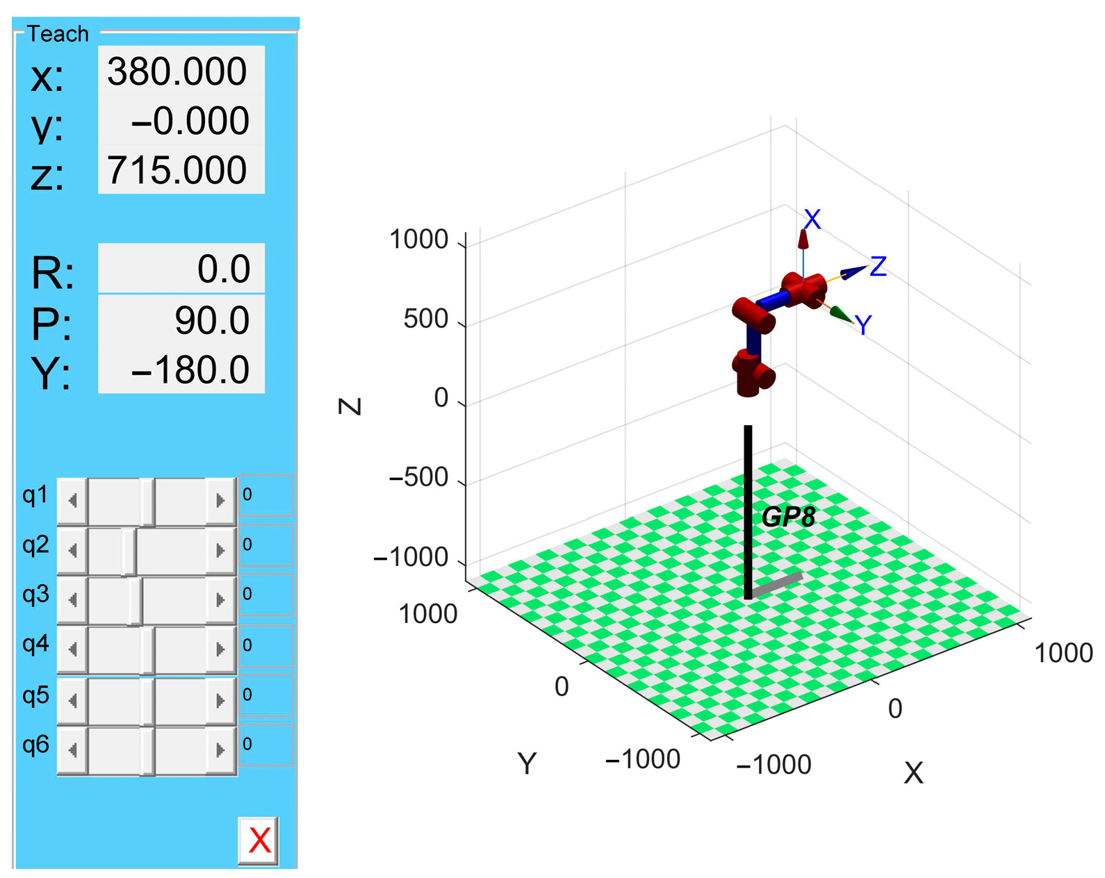
According to the DH parameters of the manipulator shown in Table 1, the motion modeling of the manipulator is carried out, and the modeling results are shown in Figure 2, the unit here is mm.

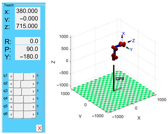
Figure 2. Motion modeling diagram of the GP8 manipulator.

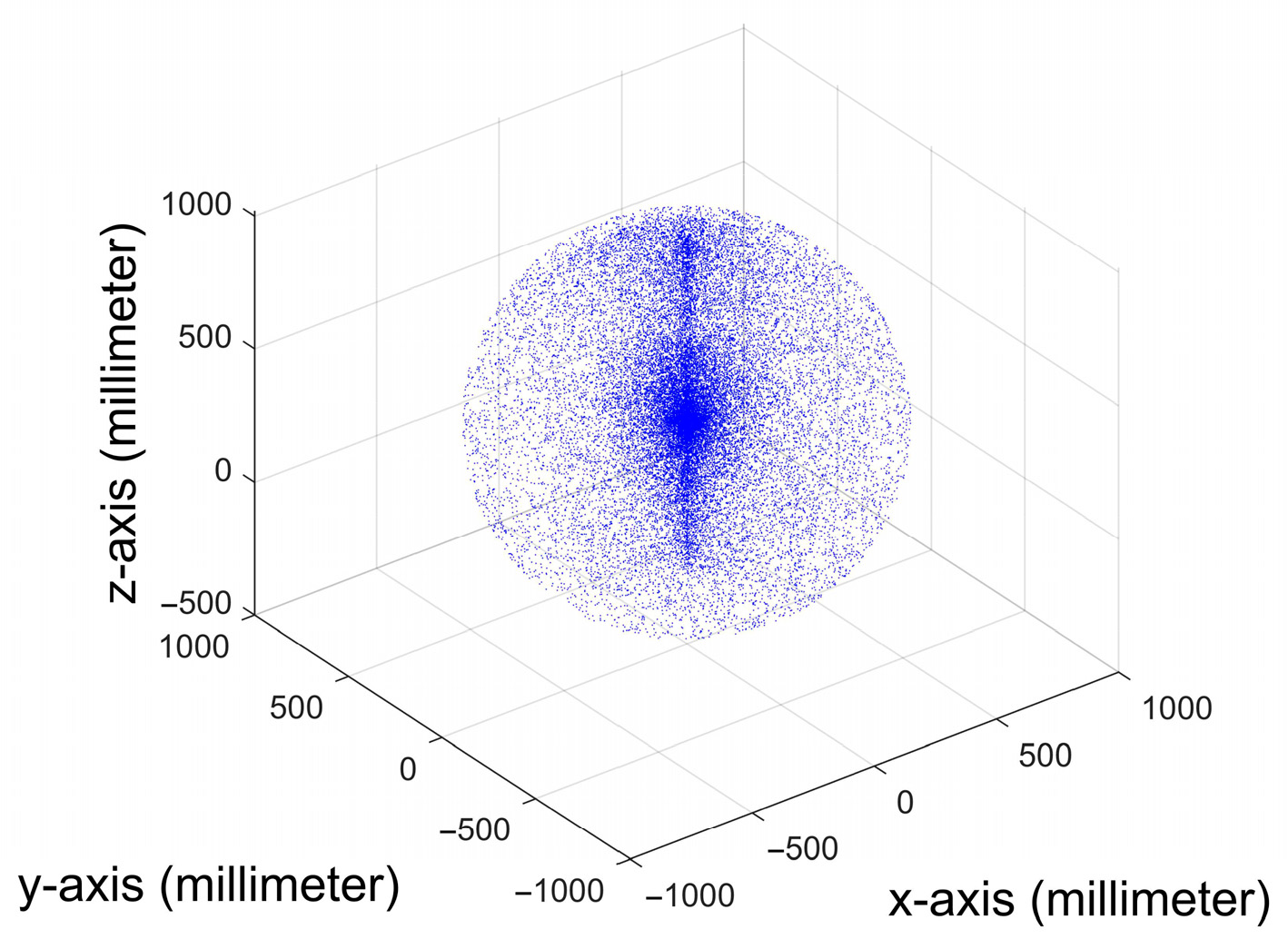
The Monte Carlo method is used to solve the motion space of the manipulator. The basic idea of the algorithm is that each joint of the manipulator is randomly traversed within the motion limit range, and the space is discretized by its forward kinematics mapping. The set of all random values of the end effector in the space constitutes the workspace of the manipulator.

The specific steps are as follows:

Step1: Within the limit of the motion range of each joint of the manipulator, the random number rand (N, 1) in the interval of [0, 1] is generated by a random function, and the random value of each joint is calculated:

$${\theta }_i={\theta }_{i\min }+rand(N,1)\times ({\theta }_{i\max }-{\theta }_{i\min })$$

(10)

In formula (10), N is the number of random numbers and ${\theta }_i$ is the i-th joint angle, ${\theta }_i\in \left[{\theta }_{i\min },{\theta }_{i\max }\right]$.

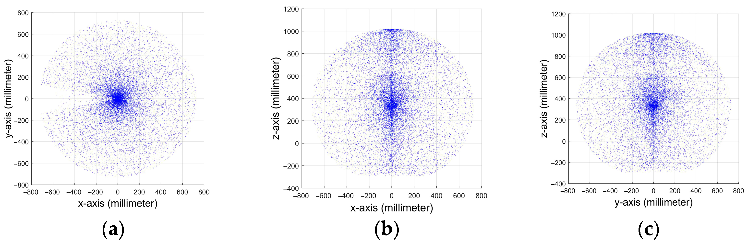
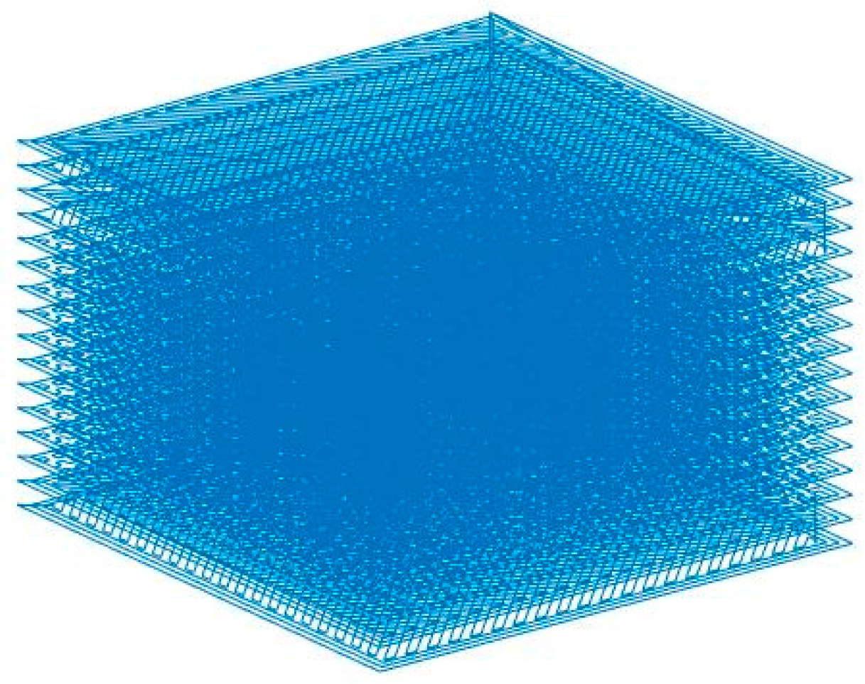
Step2: The pseudo-random value ${\theta }_i$ solved in Step1 is substituted into the obtained forward kinematics equation of the manipulator to obtain the position point of the end effector of the manipulator in space. The set of end effectors corresponding to the random values of all joints in space points can be obtained by reciprocating circulation, and the workspace of the corresponding manipulator can be obtained. The motion space of the GP8 manipulator is shown in Figure 3.

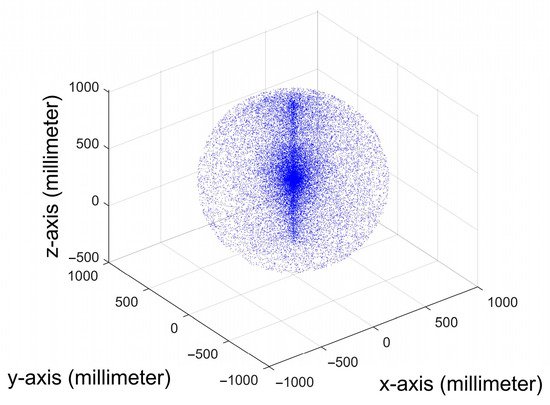
Figure 3. Motion space of the GP8 manipulator.

Figure 4a is the xoy section projection of the manipulator motion space, Figure 4b is the xoz section projection of the manipulator motion space, and Figure 4c is the yoz section projection of the manipulator motion space. $X\in [-709.3663,725.1195]$, $Y\in [-721.4648,725.2185]$, and $Z\in [-293.7268,1017.3194]$.

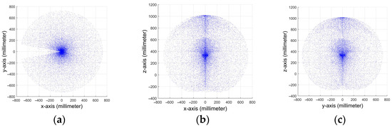
Figure 4. Motion space cross-section projection of the GP8 manipulator. (a) Cross-sectional projection of xoy. (b) Cross-sectional projection of xoz (c) Cross-sectional projection of yoz.

The GP8 manipulator follows the Pieper criterion, that is, the last three axes of the manipulator intersect at one point. The inverse kinematics can be solved by using this criterion to obtain the optimal solution of six joints. According to the position of the wrist of the manipulator, the angle of six joints is solved by the analytical method, and then all eight groups of solutions of the manipulator are obtained. Finally, according to the constraints of each joint, the solutions that are not within the joint range of the manipulator are deleted, and the optimal solution that meets the conditions is obtained.

Based on the above solution method, the inverse kinematics of the printing path is solved, and the printing path simulation is performed. Figure 5 is the printing path simulation.

Figure 5. Printing path simulation.

3. A Six-DOF Path Planning Algorithm Combining Contour Offset Filling Method and Improved Hilbert Curve Filling Method

3.1. The Basic Idea of the Algorithm

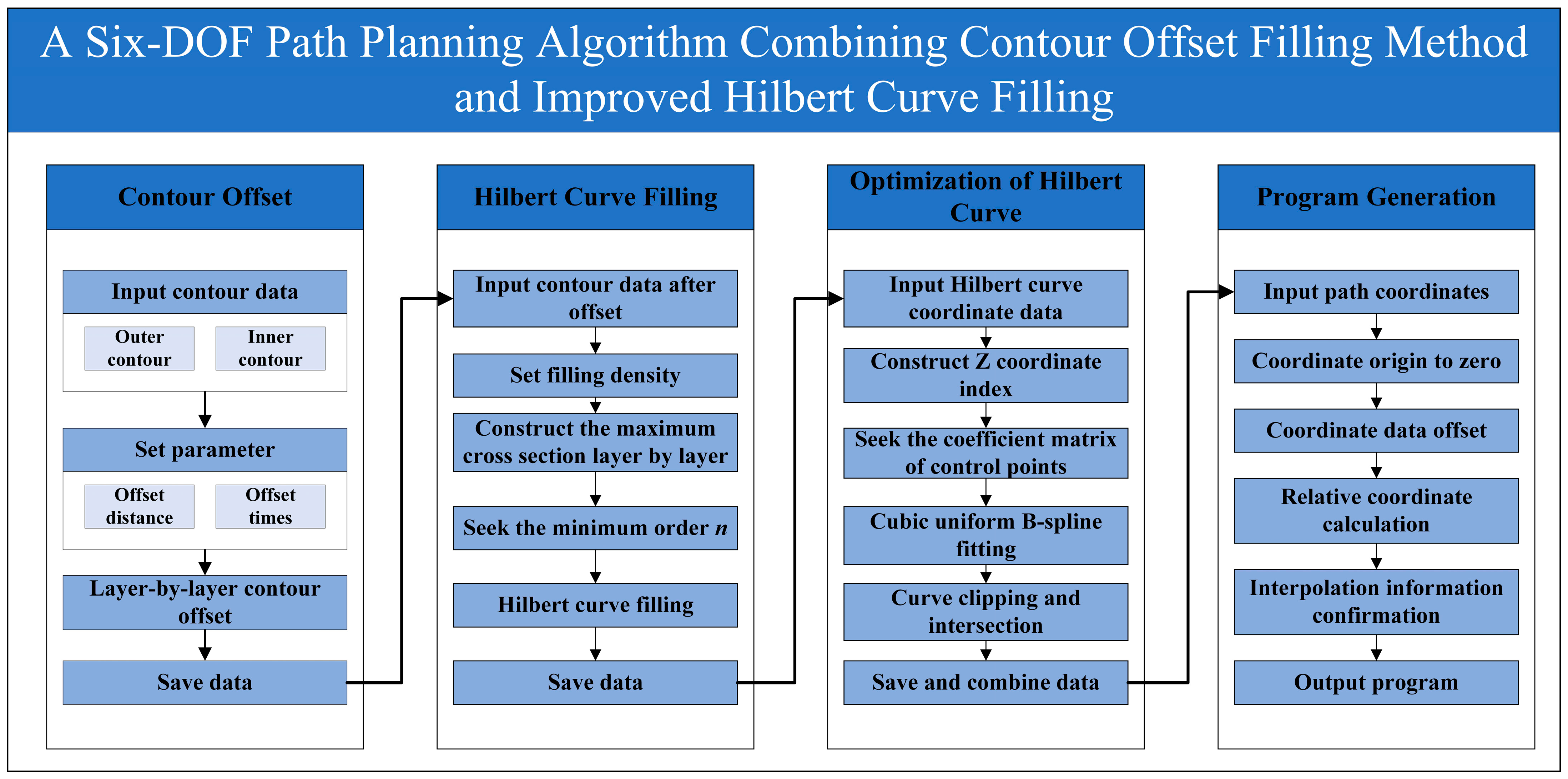
The contour offset filling method is used to fill the contour edge of the model several times, and the offset number taken in this paper is 1. The external contour is offset inward, and the internal contour is offset outward. According to the profile data after offset, the Hilbert curve is used to fill it. The cubic uniform B-spline curve is used to fit the generated Hilbert curve, and the optimization is carried out based on ensuring continuity. The overlapping part and the out-of-bounds part are processed. Finally, the manipulator program is generated.

3.2. The Basic Principle of the Algorithm

3.2.1. Hilbert Curve

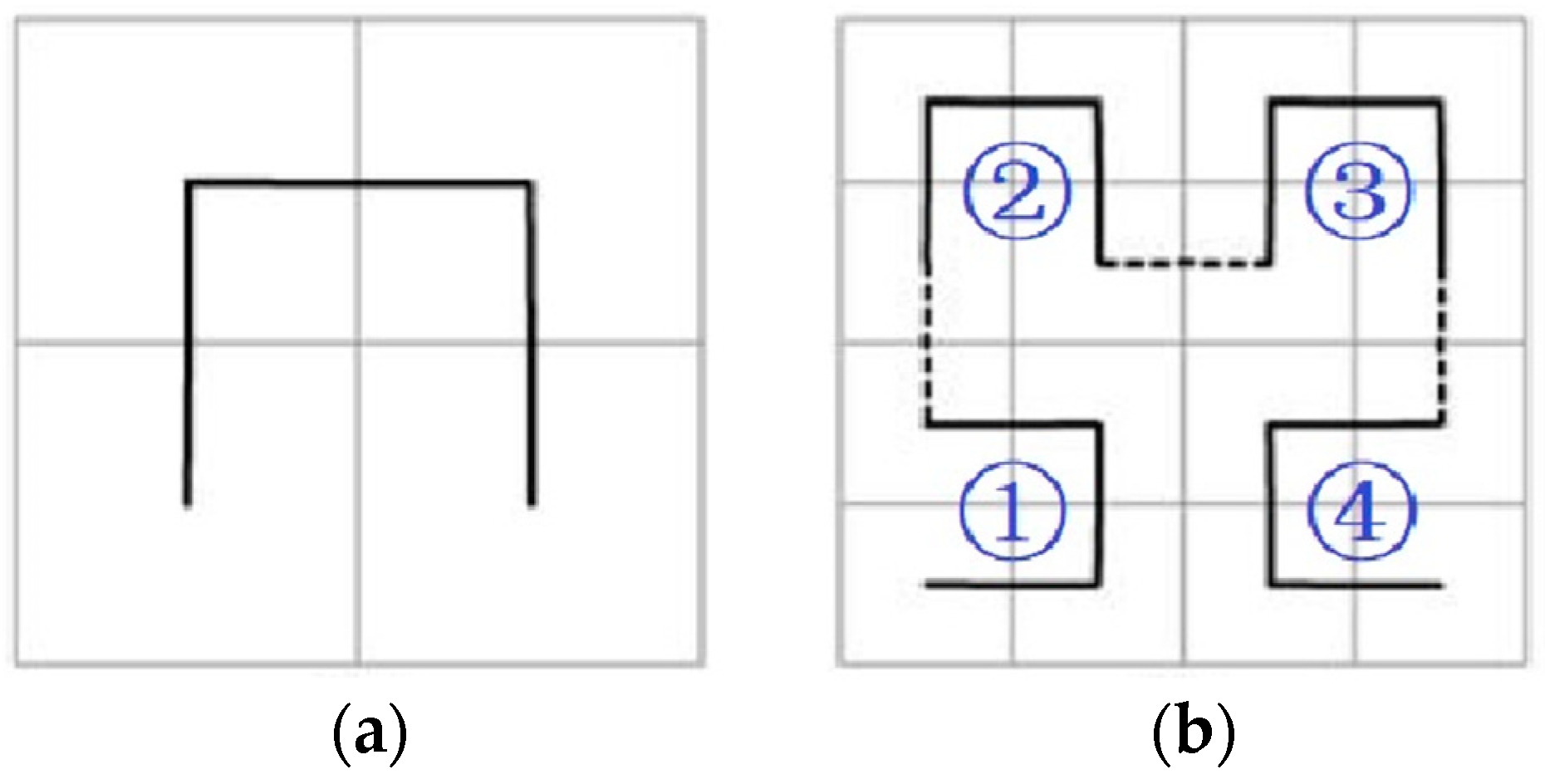
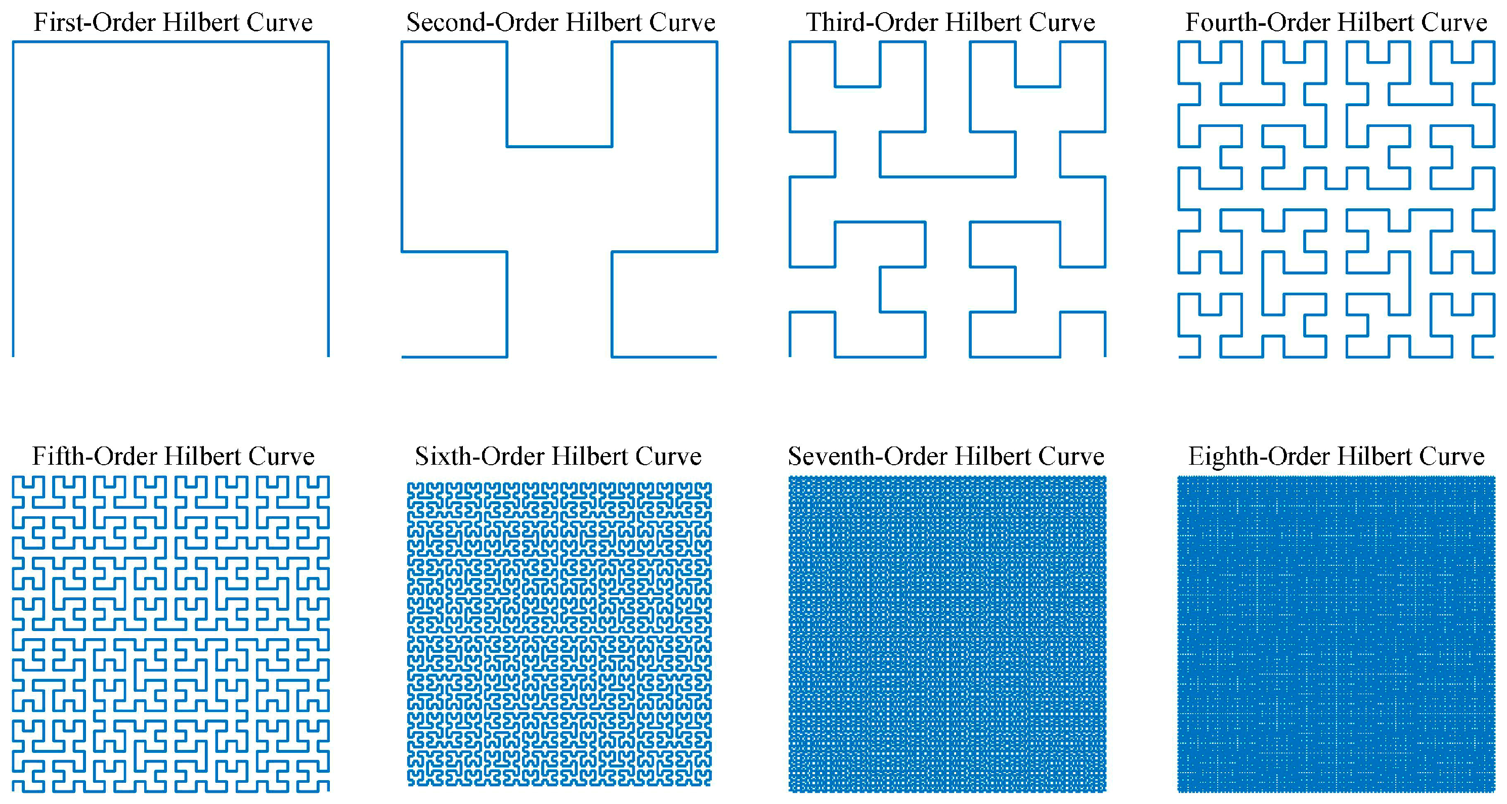
The Hilbert curve is a fractal curve that is a continuous, self-avoiding, filled unit square curve. The definition of the Hilbert curve is to divide a unit square into $2^n\times 2^n$ small equal squares of equal size. The side length of each small square is $1/2^n$, where n is the order of the Hilbert curve. Small squares are numbered from small to large in a certain order. The center points of small squares are connected with curves in order to obtain the corresponding order Hilbert curve [19]. Figure 6 is a diagram of the change process of the Hilbert curve. The change process of the second-order Hilbert curve is as follows:

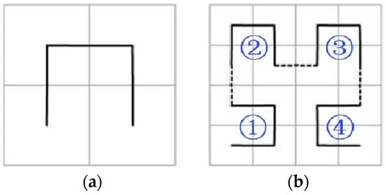
Figure 6. The change process of the Hilbert curve: (a) first-order Hilbert curve and (b) second-order Hilbert curve.

Step1: Copy four copies of the first-order Hilbert curve graph shown in Figure 6a;

Step2: Flip the two first-order Hilbert curves of the lower left corner ① and the lower right corner ④;

Step3: Connect and form the second-order Hilbert curve, as shown in Figure 6b.

Similarly, the n-order Hilbert curve is based on the n − 1-order Hilbert curve for Step1–Step3.

3.2.2. Cubic Uniform B-spline Curve

The B-spline curve segment is defined by a series of control points and node vectors. The node vector determines the parameter values on the curve, and the control points determine the shape of the curve. The fitting process of the cubic uniform B-spline function is as follows: firstly, the coordinates of all points of the original curve are input, and the cubic B-spline smoothing is carried out. The given points are smoothed to the B-spline curve without increasing the number of points. Then, the cubic uniform B-spline fitting is performed, and a specified number of points are uniformly inserted between the nodes to complete the fitting. Given n + 1 control points $V_i(i=0,1,2,\mathrm{\dots },n,n\ge 3)$, the r-degree B-spline function can be defined as follows:

$$P(u)={\displaystyle \sum _{i=0}^n{B}_{i,r}}(u)V_i,u_r\le u\le u_{r+1}$$

(11)

where $B_{i,r}(u)$ is the basis function of the B-spline function of degree r, where $u\in [0,1]$.

By the De Boor recursive formula [20]:

$$\left\{\begin{array}{l}{B}_{i,0}(u)=\left\{\begin{array}{l}1,u\in [u_i,u_{i+1}]\hfill \\ 0,othervise\hfill \end{array}\right.\hfill \\ B_{i,r}(u)=\frac{u-u_i}{u_{i+r}-u_i}{B}_{i,r-1}(u)+\frac{u_{i+r+1}-u}{u_{i+r+1}-u_{i+1}}{B}_{i+1,r-1}(u),r⩾1\hfill \\ \frac{0}{0}=0\hfill \end{array}\right.$$

(12)

when the degree r is 3, the i-th trajectory can be expressed as:

$$B_{i,3}(u)=\frac{u-u_i}{u_{i+3}-u_i}{B}_{i,2}(u)+\frac{u_{i+4}-u}{u_{i+4}-u_{i+1}}{B}_{i+1,2}(u)$$

(13)

The interval of the cubic uniform B-spline is [0, 1]. Expanded by intervals, the Formula (13) becomes:

$$\left\{\begin{array}{l}{B}_{0,3}=\frac{1}{6}{(1-u)}^3\hfill \\ B_{1,3}=\frac{1}{6}\left(3u^3-6u^2+4\right)\hfill \\ B_{2,3}=\frac{1}{6}\left(-3u^3+3u^2+3u+1\right)\hfill \\ B_{3,3}=\frac{1}{6}{u}^3\hfill \end{array}\right.,u\in [0,1]$$

(14)

The cubic uniform B-spline function formula can be obtained by expanding Formula (11).

$$P(u)={\displaystyle \sum _{i=0}^3{B}_{i,3}}(u)V_i=\frac{1}{6}\left[\begin{array}{cccc}{u}^3& u^2& u& 1\end{array}\right]\left[\begin{array}{cccc}-1& 3& -3& 1\\ 3& -6& 3& 0\\ -3& 0& 3& 0\\ 1& 4& 1& 0\end{array}\right]\left[\begin{array}{c}{V}_0\\ V_1\\ V_2\\ V_3\end{array}\right]$$

(15)

3.3. The Basic Steps and Effect Diagram of the Algorithm

The flow chart of the path planning algorithm is shown in Figure 7. The specific implementation process is as follows:

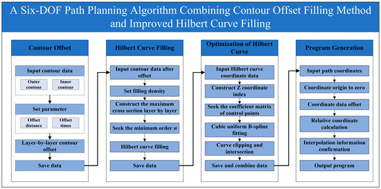
Figure 7. The flow chart of the path planning algorithm.

3.3.1. Contour Offset

The model is sliced and layered to obtain the inner contour and outer contour data of the model. The outer contour is offset inward and the inner contour is offset outward to obtain the offset contour data. Figure 8 is the contour offset effect diagram, where the red line is the outer contour and the blue line is the inner contour.

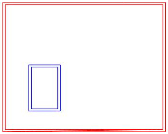
Figure 8. Contour offset.

3.3.2. Hilbert Curve Filling

The first to eighth-order Hilbert curves obtained by MATLAB programming are shown in Figure 9. The area of each order Hilbert curve is $(2^n-1{)}^2$. Therefore, the area of the offset contour is as follows:

$$A=(X_{\max }-X_{\min })\times (Y_{\max }-Y_{\min })$$

(16)

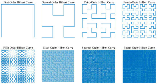
Figure 9. The first to eighth-order Hilbert curves.

The minimum order n of the Hilbert curve of the current offset contour is calculated by Formula (17).

$$(2^n-1{)}^2\ge A$$

(17)

The above formula is equivalent to the following formula.

$$n\ge {\log }_2(\sqrt{A}+1)$$

(18)

The Hilbert curve of the corresponding order is generated to complete the filling of the offset contour.

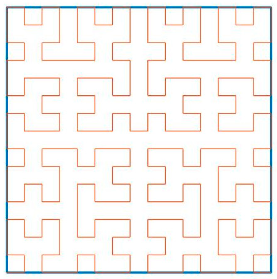
According to the cross-section data, the Hilbert curve is used to fill the model, and the filling effect is shown in Figure 10. The blue line is the offset contour, and the orange line is the Hilbert curve.

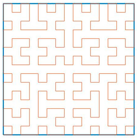
Figure 10. The filling effect.

3.3.3. Optimization of the Hilbert Curve

• Cubic Uniform B-spline Fitting

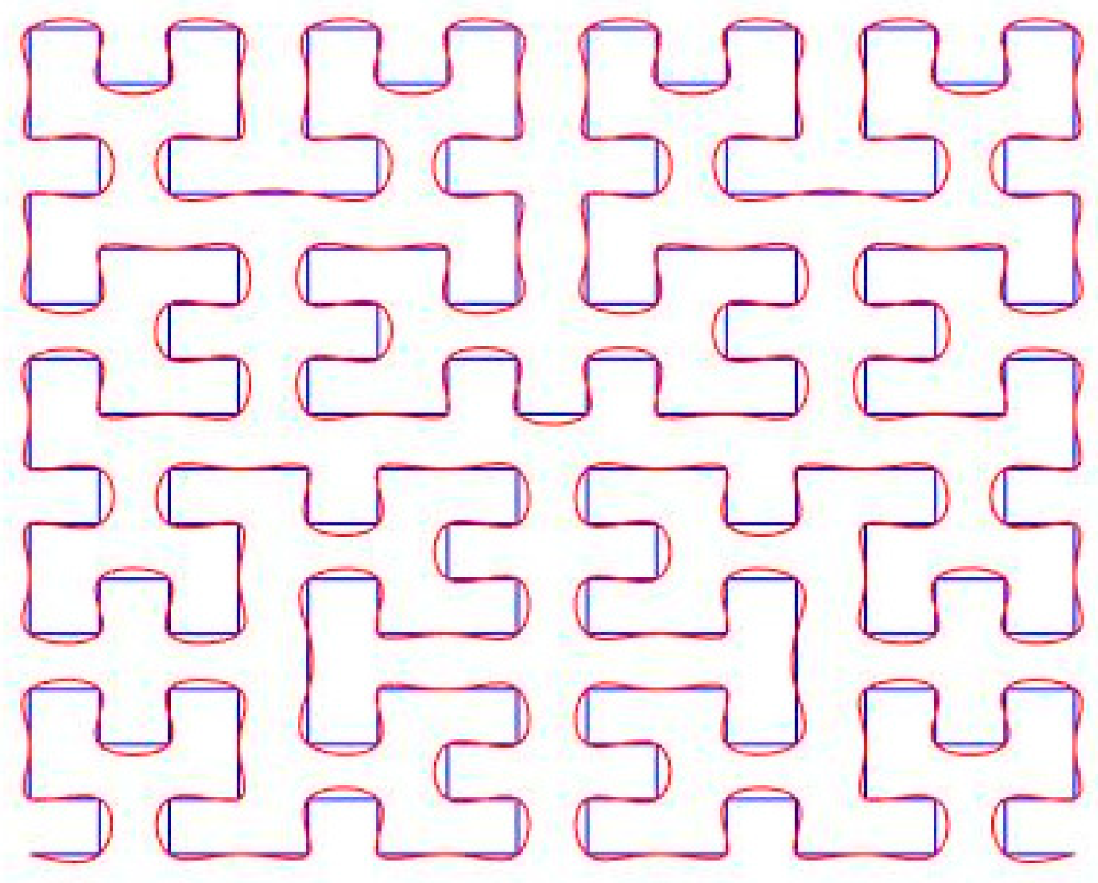
According to the generated Hilbert curve coordinates, the control points of the cubic uniform B-spline curve are obtained, and the fitting curve is constructed. The curve after interpolation fitting of the Hilbert curve using the cubic uniform B-spline function is shown in Figure 11. The blue solid line is the original Hilbert curve, and the magenta solid line is the fitting curve.

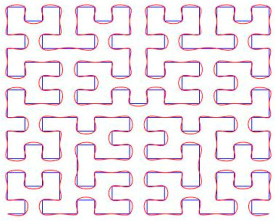
Figure 11. Original curve and fitting curve.

2.

Curve Clipping and Intersection

The polygonal Boolean operation is used to complete the clipping of the fitting Hilbert curve and the model contour. The coordinate point data of the optimized Hilbert curve is stored in array A, the outer contour data of the model is stored in array B, and the inner contour data of the model is stored in array C.

Firstly, the Hilbert curve beyond the outer contour is truncated. The intersection of array A and array B is obtained by using polygon Boolean operation, and the truncated data is stored in array D.

$$D=A\cap B$$

(19)

Then, the Hilbert curve inside the inner contour is intersected. The difference set of arrays C and D is obtained, and the intercepted data is stored in array E.

$$E=D-C$$

(20)

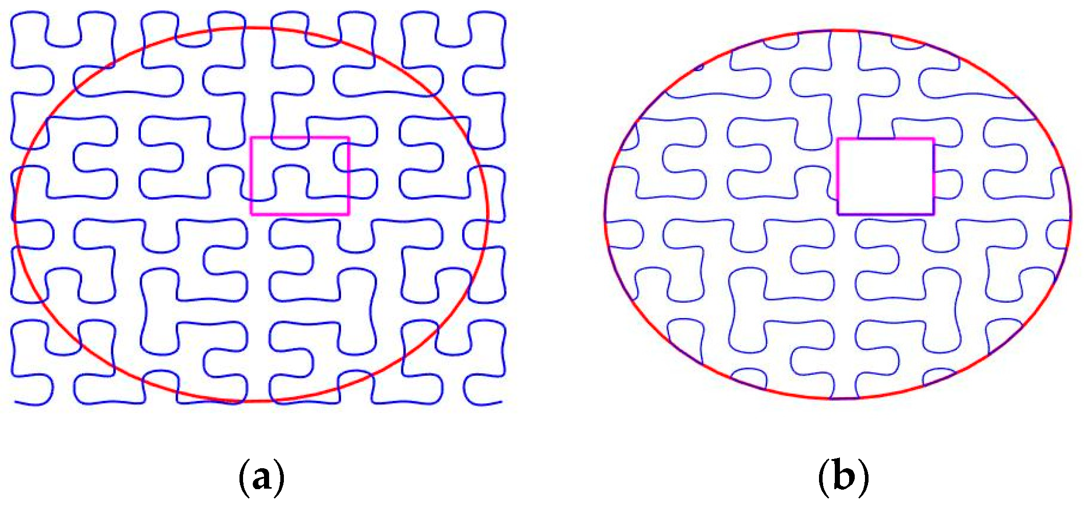
Figure 12a is the filling effect diagram without curve clipping and intersection, and Figure 12b is the filling effect diagram after curve clipping and intersection. In Figure 12, the red curve is the outer contour, the blue curve is the optimized Hilbert curve after the intersection, and the magenta curve is the inner contour.

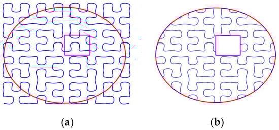
Figure 12. Curve clipping and intersection diagrams: (a) the filling effect diagram without curve clipping and intersection and (b) the filling effect diagram after curve clipping and intersection.

3.

Data Integration

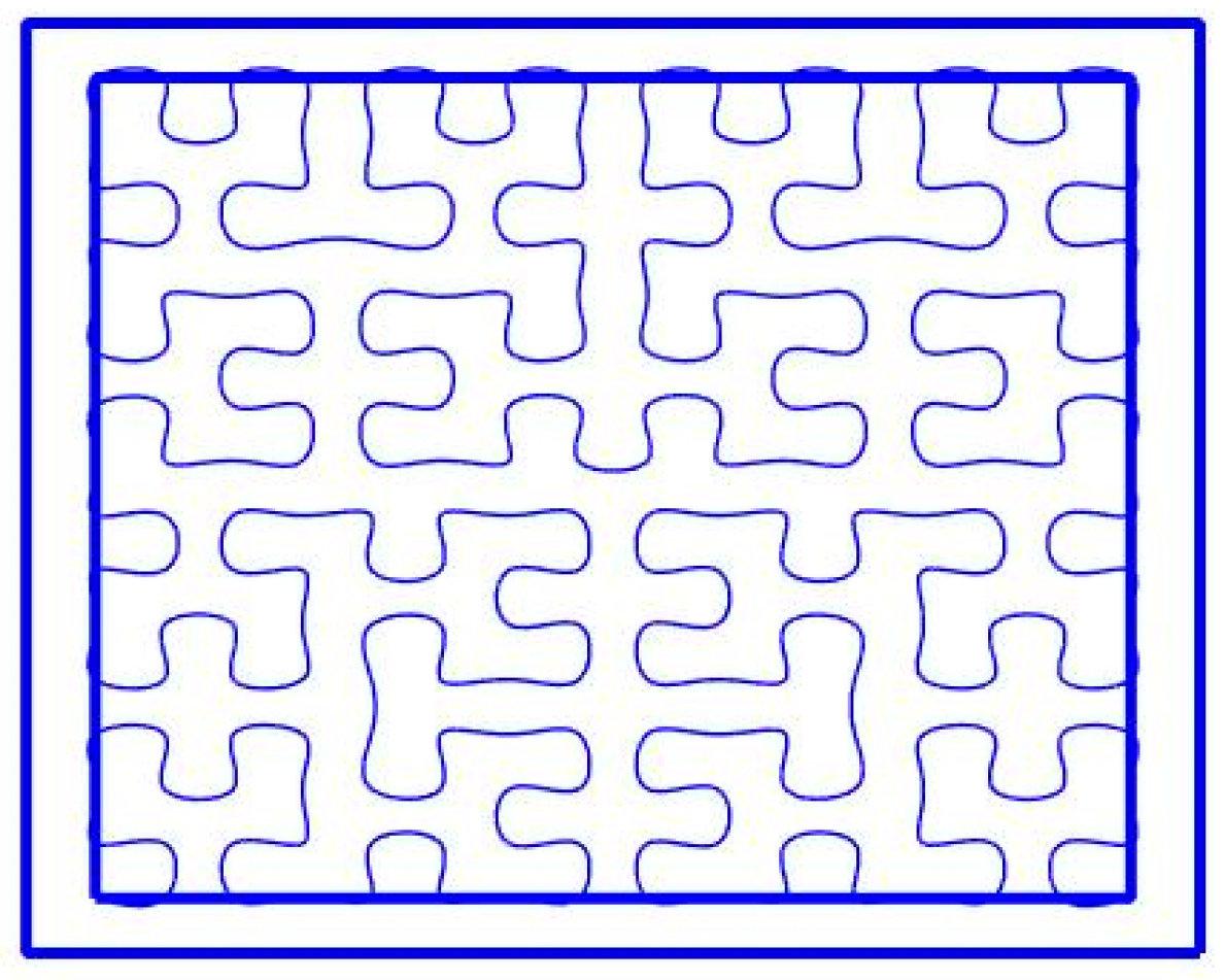
The contour data of each layer is integrated with the internal filling data to obtain the printing path point data. The printing path effect diagram is shown in Figure 13.

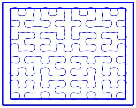
Figure 13. The printing path effect diagram.

3.3.4. Program Generation

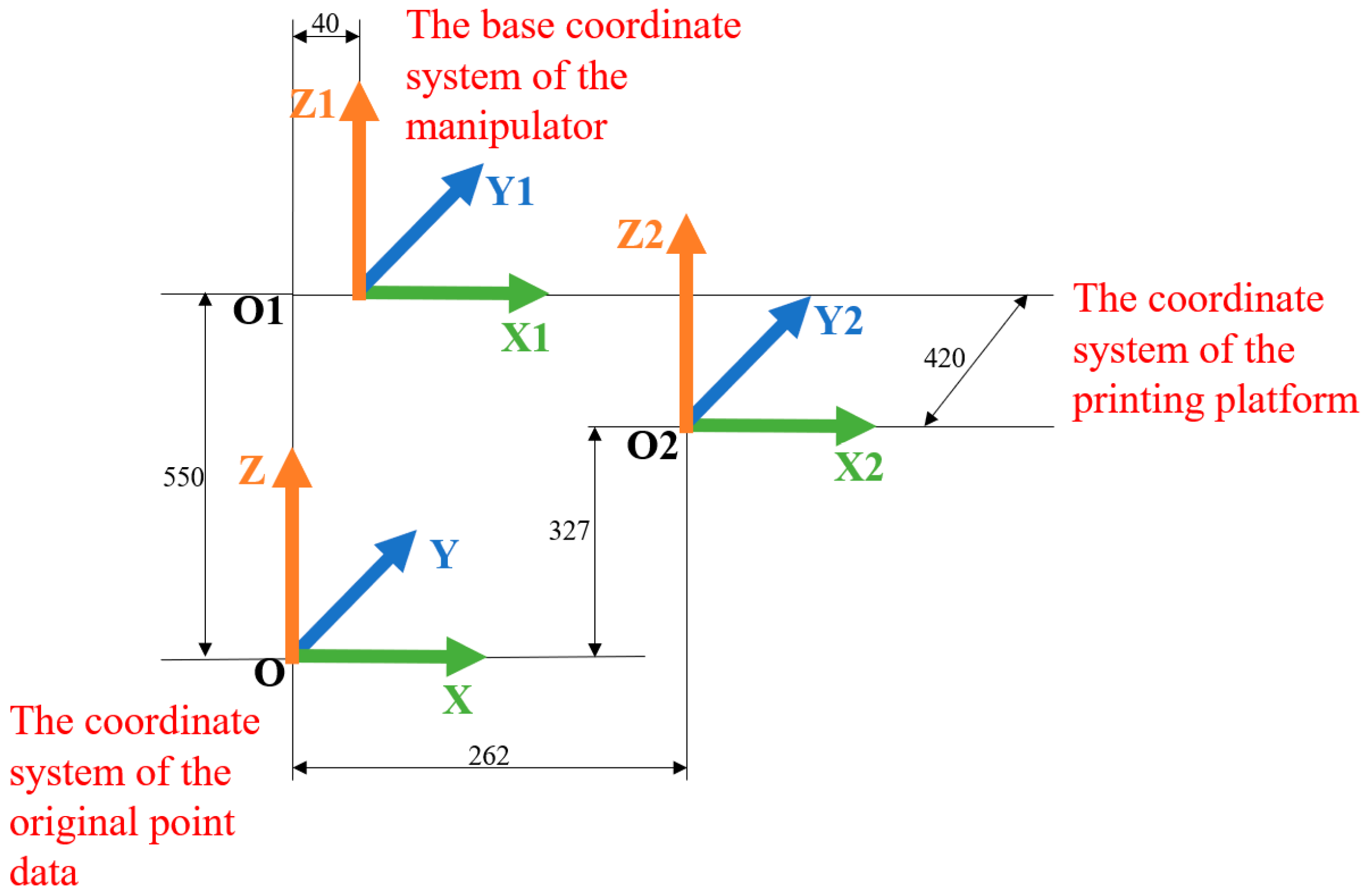
According to the format requirements of the associated mode program, it is necessary to convert the coordinates of the printing path points into the coordinates of the printing path in the printing platform relative to the base coordinate system of the manipulator. The position relationship between the coordinate system of the original point data, the coordinate system of the printing platform, and the base coordinate system of the manipulator is shown in Figure 14, the unit here is mm.

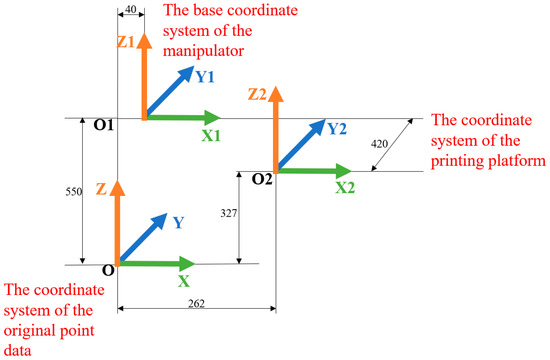
Figure 14. Schematic diagram of coordinate transformation coordinate system pose relationship.

The specific steps of data conversion and program generation are as follows:

Step1: Coordinate origin to zero. In order to ensure the accuracy of coordinate transformation, before coordinate transformation, the starting coordinate origin of this group of coordinate data should be set to (0, 0, 0). The specific operation is to take the minimum value of the three coordinates in the first layer of the model as the zero point so that the minimum value of the component layer data is subtracted, that is, the zeroing operation is completed.

Step2: Coordinate data offset. After Step1 processing, the data after the coordinate origin is zeroed are obtained, and the newly obtained data are offset to the coordinate system of the printing platform.

Step3: Relative coordinate calculation. According to the relative position relationship between the base coordinate system of the manipulator and the coordinate system of the printing platform, the relative coordinates of the coordinate system of the printing platform and the base coordinate system of the manipulator are obtained.

Step4: Interpolation information confirmation. Interpolation information mainly includes interpolation point coordinates, interpolation angle, interpolation method, and interpolation speed. Interpolation point coordinates are obtained by Step1–Step3. The interpolation angle is determined according to the angle between the normal vector of the current printing plane and the Z-axis of the base coordinate system. The interpolation methods of the GP8 manipulator mainly include joint interpolation, linear interpolation, arc interpolation, and free curve interpolation. Because of the large number of point data, the manipulator is prone to alarm when using circular interpolation and free curve interpolation, which will cause the manipulator to stop running. Joint interpolation will produce trajectory offset during the printing process, so the interpolation method combining joint interpolation and linear interpolation is selected. Joint interpolation is used before entering the initial point of printing and after the end point of printing, and linear interpolation is used during the printing process. Through experimental comparison and material properties, the joint interpolation speed is set to 0.78% (the joint interpolation speed is expressed as a ratio to the highest speed), and the linear interpolation speed is 23.0 mm/s.

4. Experiment and Discussion

In order to verify that the six-DOF AM platform is more efficient than the traditional AM device in model printing, the models are printed on the traditional three-axis AD device and the six-DOF AM platform by using the parallel scanning filling method. The printing time is compared.

In order to verify the effectiveness and practicability of the proposed method, experiments are carried out. Firstly, the model is sliced hierarchically to obtain contour data. Secondly, the parallel scanning filling method, the path planning algorithm combining contour offset and Hilbert curve, and the method proposed in this paper are used for path planning. Then, simulation software is used to improve printing path programs and convert print programs. Finally, the six-DOF AM platform is used to complete the printing of multiple models, and the three-coordinate measuring instrument is used to detect the degree of warpage deformation of the models filled by the three methods.

4.1. Printing Path Program Improvement and Program Conversion

Simulation software is used to build the simulation environment, and the improvement in the printing path program and the program conversion are completed in the simulation environment. Through the algorithm steps described in Section 3.3, the printing path program can be obtained. Using the simulation environment to improve the printing path program, it is necessary to control the consumables conveying mechanism to obtain the printing program. Because the manipulator of this printing platform is limited by the program format, it is necessary to convert the associated mode program into the standard mode program.

4.1.1. Improving the Printing Path Program

For the motor control of the consumables conveying mechanism, the I/O signal is used to start and stop the control. OT# (2) is the start signal and OT# (3) is the end signal. The start signal is added before the start of model printing, and the end signal is added after the end of model printing.

In order to ensure the uniformity of the printing sprinkler head during printing, it is necessary to add free distance outside the printing model range before the printing program starts to avoid the lack of consumables supply during the printing process.

The single program of the GP8 manipulator can accommodate up to 9998 interpolation points. Because of the large number of printing path points generated by the method in this paper, the program needs to be split when generating the program, and each program is connected in series by CALL statement.

4.1.2. Standard Mode Program Generation

The GP8 manipulator program can be divided into two categories as follows: the associated mode program and the standard mode program. The point data format in the associated mode program is the coordinates and angles relative to the base coordinate system, and the point data format in the standard mode program is the pulse value of each joint.

The converted standard pattern program is shown in Figure 15, where 0418A011 is the printing path program.

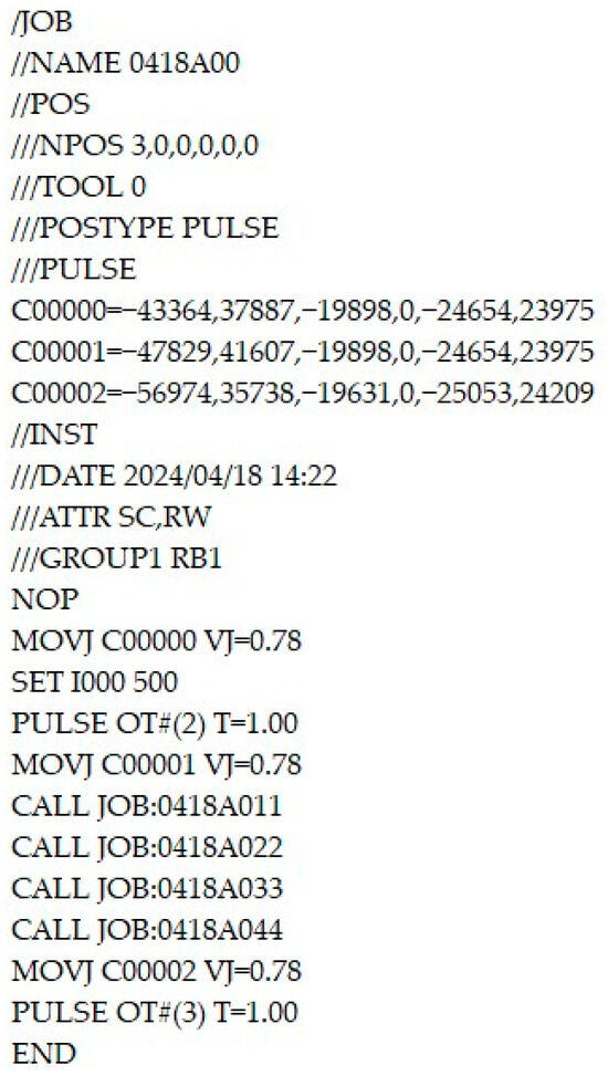
Figure 15. Standard mode program.

4.2. Model Printing and Result Analysis

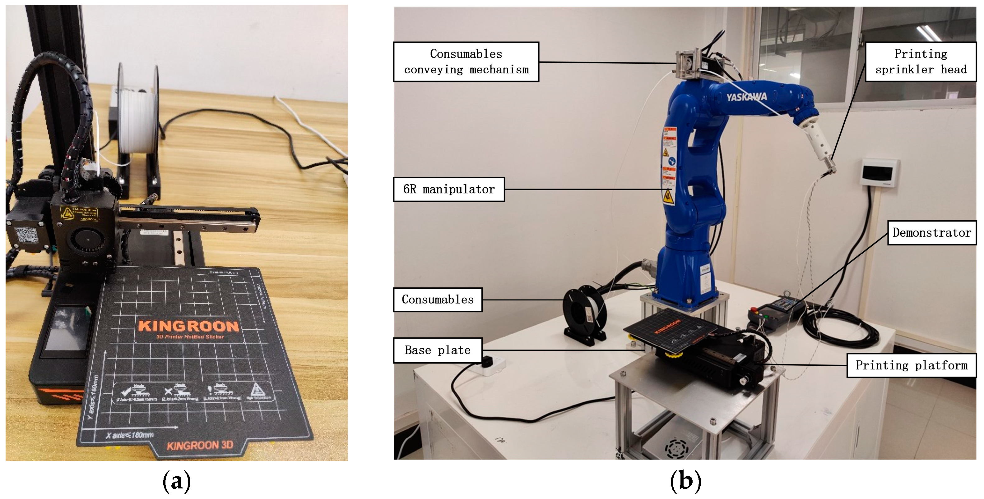
Two additive manufacturing devices are shown in Figure 16. The main specifications of the six-DOF AM platform are shown in Table 2.

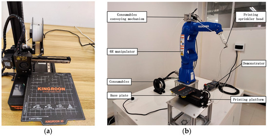
Figure 16. Additive manufacturing devices: (a) a traditional 3-axis AM device and (b) the 6-DOF AM platform.

Table 2. The main specifications of the 6-DOF AM platform.

Name	Parameter
Mechanical arm	Yaskawa GP8
Consumable conveying mechanism	SGM7J-04APK-YR11
Control cabinet inspection	YR1000
Consumable materials	PLA (polylactic acid)
Diameter of consumables	1.75 mm
The diameter of printing sprinkler head	0.4 mm

The molding temperature is 25 °C, the temperature of the printing sprinkler head is 200 °C, the printing platform temperature is 60 °C, the layer thickness is 0.2 mm, and the filling density is 100%. With PLA as the printing material, the cube model with a size of 63 × 63 × 4 (mm) and the cylinder model with a radius of 30 (mm) and a height of 4 (mm) are filled by the parallel scanning filling method. The traditional three-axis additive manufacturing device and the six-DOF AM platform are used to print the two kinds of models each. In order to ensure the fairness of the experiment, the moving speed of the printing sprinkler head and the diameter of the printing sprinkler head are consistent. The model printing time (excluding the pre-planning algorithm time) is shown in Table 3.

Table 3. Model printing time (unit: h).

Model	Traditional Three-Axis AM Device	Six-DOF AM Platform
cube model	1.79	1.00
	1.78	1.01
cylinder model	1.26	0.79
	1.27	0.78

The traditional three-axis AM device prints two kinds of models, and the average time is 1.785 h and 1.265 h, respectively. The six-DOF AM platform prints two kinds of models, and the average time is 1.005 h and 0.785 h, respectively. Compared with the traditional three-axis AM device, the printing time of the six-DOF AM platform is shortened by 43.70% and 37.94%, respectively. The main reason for the difference between the two devices is that the response speed of the motor is different. When the corner is encountered, the motor response speed of the six-DOF AM device is faster, so the overall printing time is shorter, and the printing efficiency is higher.

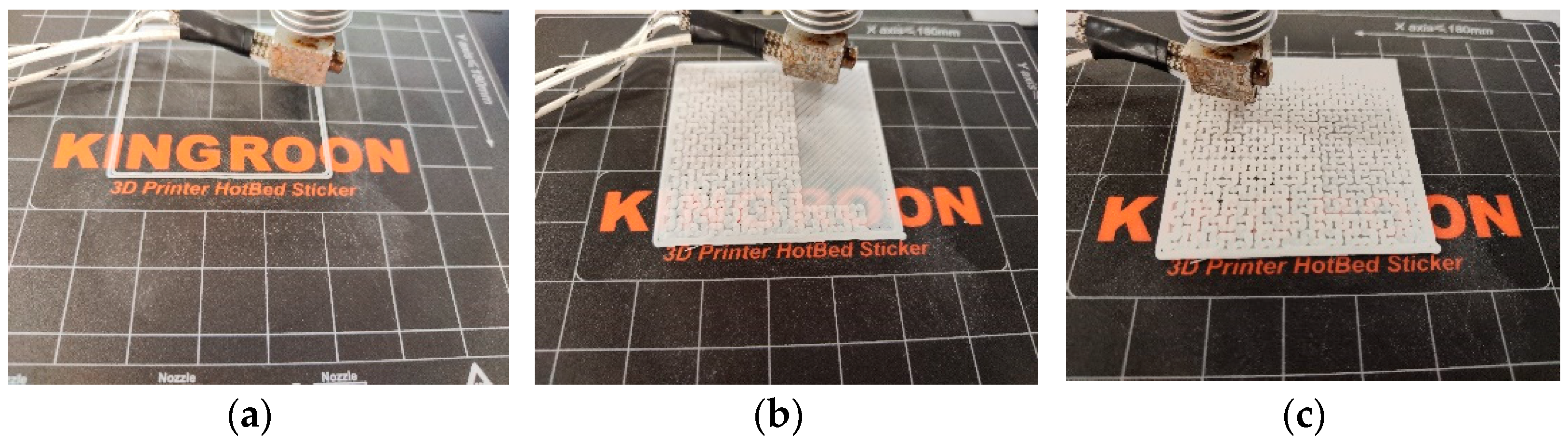
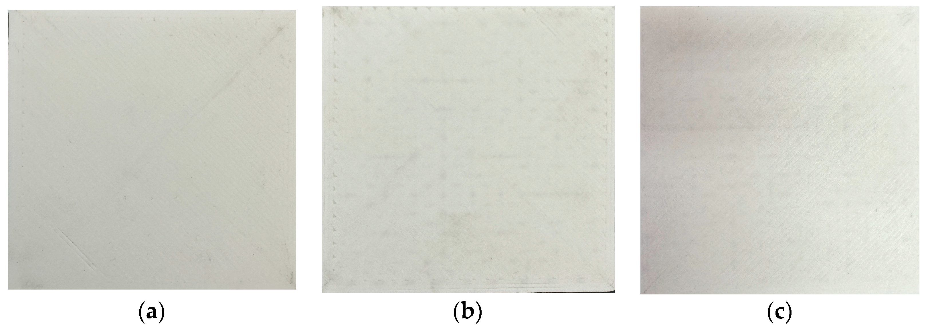
Under the above experimental conditions, the parallel scanning filling method, the path planning algorithm combining the contour offset filling method and the Hilbert curve, and the method proposed in this paper are used to fill the cube model with a part size of 63 × 63 × 4 (mm), and the six-DOF AM platform is used for printing. Three models are printed for each method. The printing process is shown in Figure 17. Comparing the printing effect, the model printing effect of the three methods is shown in Figure 18.

Figure 17. Model printing process. (a) Contour offset filling. (b) The optimized Hilbert curve is filled once. (c) The optimized Hilbert curve is filled 3 times.

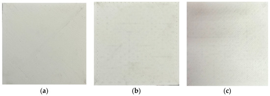
Figure 18. Experimental model. (a) The parallel scanning filling method. (b) The contour offset filling method combined with the Hilbert curve filling method. (c) The method proposed in this paper.

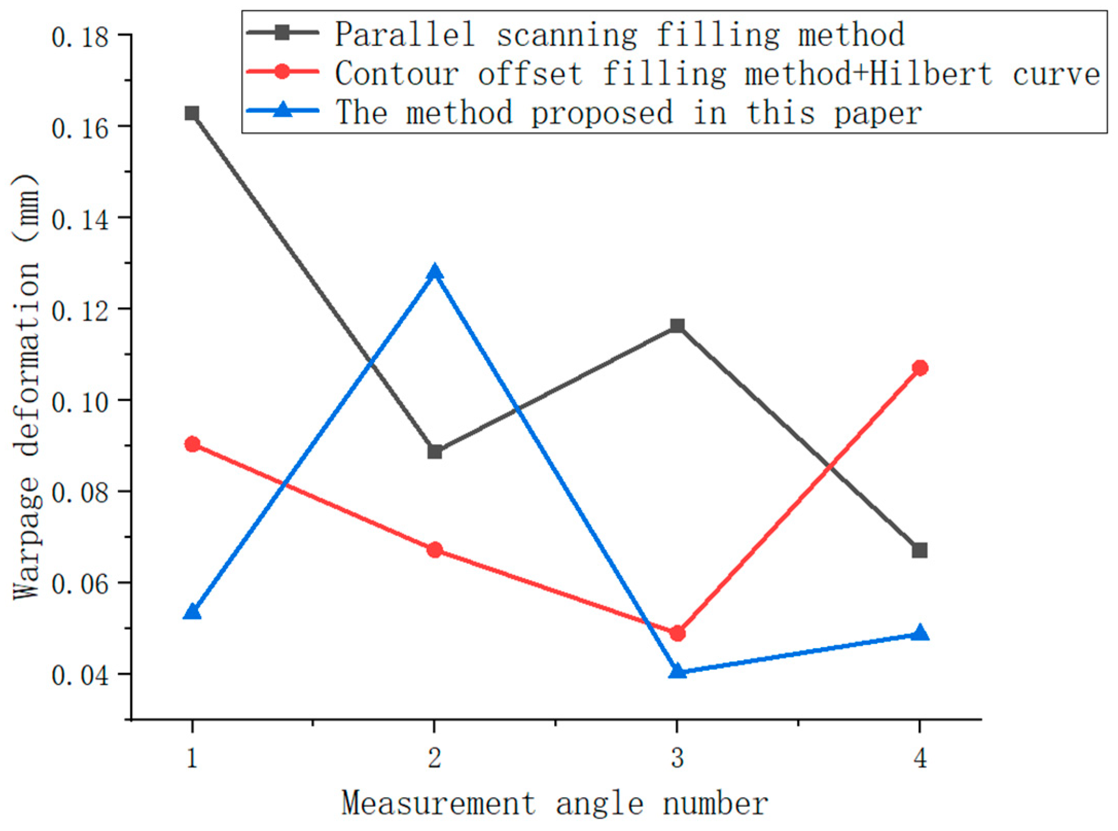
Based on the Z coordinate of the midpoint at the bottom of the model, the Z coordinate values of the four corners at the bottom of the model are measured by the three-coordinate measuring instrument. Nine points are taken from each corner, and the average value is taken as the warpage deformation of the corner. The three-coordinate measuring instrument is shown in Figure 19. The experimental results are shown in Table 4, Table 5 and Table 6, where angle 1, angle 2, angle 3, and angle 4 are the measurement angle numbers. Table 7 is the average warpage deformation of the model filled by the three different methods. Figure 20 is the average warpage deformation change diagram of the four corners of the three filling methods. It can be seen in Figure 20 that the model filled by the method proposed in this paper is superior to the model filled by the other two filling methods as a whole.

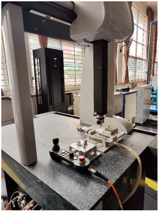
Figure 19. The three-coordinate measuring instrument.

Table 4. The warpage deformation of the model filled by the parallel scanning filling method (unit: mm).

Model Number	Angle 1	Angle 2	Angle 3	Angle 4
1	0.013603	0.159130	0.116842	0.146750
2	0.251418	0.034296	0.137811	0.029134
3	0.223515	0.072731	0.093952	0.025362

Table 5. The warpage deformation of the model filled by the contour offset filling method combined with the Hilbert curve path planning algorithm (unit: mm).

Model Number	Angle 1	Angle 2	Angle 3	Angle 4
1	0.105696	0.085047	0.069962	0.071978
2	0.086255	0.061056	0.021139	0.134344
3	0.079237	0.0556	0.055751	0.115078

Table 6. The warpage deformation of the model filled by the method proposed in this paper (unit: mm).

Model Number	Angle 1	Angle 2	Angle 3	Angle 4
1	0.014343	0.055793	0.035413	0.021405
2	0.104924	0.250106	0.044613	0.067445
3	0.041005	0.077806	0.040965	0.057535

Table 7. The average warpage deformation of the model filled by three different methods (unit: mm).

Filling Method	The Parallel Scanning Filling Method	The Path Planning Algorithm Combining the Contour Offset Filling Method	The Method Proposed in This Paper
The average warpage	0.108712	0.078429	0.067613

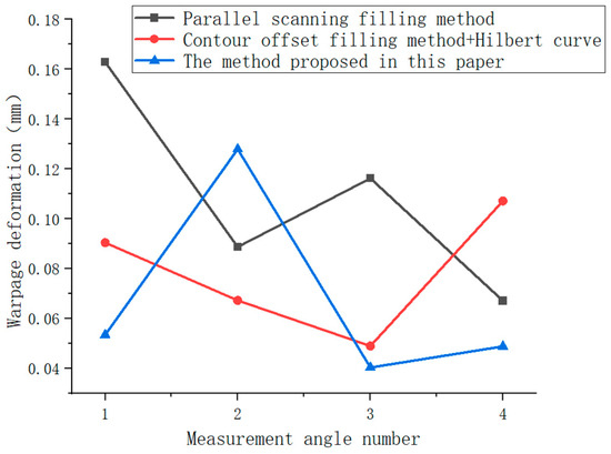
Figure 20. The average warpage deformation of the model.

It can be seen from the data in Table 7 that the average warpage deformation of the filling model of the parallel scanning filling method is 0.108712 mm, the average warpage deformation of the filling model of the path planning algorithm combining the contour offset filling method and the Hilbert curve is 0.078429 mm, and the average warpage deformation of the filling model of the proposed method is 0.067613 mm. Compared with the other two methods, the warpage deformation of the model filled with the proposed method is reduced by 37.81% and 13.79%, respectively. The degree of warpage deformation is affected by the cooling rate of the model, the thickness of the model, and the force of the model when the model is taken out. The slower the cooling rate of the model, the smaller the warpage deformation; the larger the thickness of the model, the smaller the warpage deformation; when the model is taken out, the more uniform the external force on the model is, the smaller the warpage deformation is.

5. Conclusions

In this paper, the six-DOF manipulator is taken as the object to study the path planning mechanism of six-DOF AM. The path planning method combining the contour offset filling method and Hilbert curve filling is optimized by using a cubic uniform B-spline curve, and a six-DOF path planning algorithm combining the contour offset filling method and improved Hilbert curve filling is obtained. The six-DOF AM platform is built and related experiments are carried out. The experimental results show that:

• Compared with the traditional three-axis AM device, when the six-DOF AM platform is used for model printing, the printing time is reduced by 43.70% and 37.94%, respectively, and the molding efficiency is significantly improved.
• Compared with the parallel scanning filling method and the path planning algorithm combining contour offset and the Hilbert curve, the average warpage deformation degree of the model filled by the method proposed in this paper is reduced by 37.81% and 13.79% respectively. Model printing by the method proposed in this paper improves the molding quality of the model to a certain extent.

In the future, the six-DOF AM platform will be further optimized to give full play to the flexibility of the six-DOF manipulator. For models with complex surfaces, the related hierarchical algorithms will be studied in the future, and the path planning algorithm will be further optimized to improve printing efficiency and realize unsupported printing. Some new methods will be used to solve the existing problems, such as multilayer neurocentral of high-order uncertain nonlinear systems with active disturbance rejection, asymptotic tracking with novel integral robust schemes for mismatched uncertain nonlinear systems, and so on.

References

- Wu, C.; Dai, C.; Wang, C.; Liu, Y. A Review of the Research Progress of Multi-Degree-of-Freedom 3D Printing Technology. Chin. J. Comput. 2019, 42, 1918–1938. [Google Scholar] [CrossRef]
- Wang, X.; Zhu, L. Application and Development Trend of 3D Printing in the Field of New Energy Vehicle Manufacturing. Mach. Met. Form. 2022, 7, 1–6. [Google Scholar]
- Georgopoulou, A.; Egloff, L.; Vanderborght, B.; Clemens, F. A Sensorized Soft Pneumatic Actuator Fabricated with Extrusion-Based Additive Manufacturing. Actuators 2021, 10, 102. [Google Scholar] [CrossRef]
- Zeng, Y.; Liu, H.; Sha, C.; Zhou, J.; Li, H. 3D printed collagen-based materials and their application in oral tissue regeneration and repair. Leather Sci. Eng. 2023, 33, 47–54. [Google Scholar] [CrossRef]
- Joshi, S.C.; Sheikh, A.A. 3D printing in aerospace and its long-term sustainability. Virtual Phys. Prototy 2015, 10, 175–185. [Google Scholar] [CrossRef]
- Lu, X. Research on the Application of 3D Printing Technology in the Cultivation of Mechanical Students in Higher Vocational Colleges. Auto Time 2023, 22, 46–48. [Google Scholar] [CrossRef]
- Jin, Y.; He, Y.; Xue, G.; Fu, J. A parallel-based path generation method for fused deposition modeling. Int. J. Adv. Manuf. Tech. 2015, 77, 927–937. [Google Scholar] [CrossRef]
- Yang, Y.; Loh, H.T.; Fuh, J.Y.H.; Wang, Y.G. Equidistant path generation for improving scanning efficiency in layered manufacturing. Rapid Prototyp. J. 2002, 8, 30–37. [Google Scholar] [CrossRef]
- Yu, S.; Zhang, F.; Tan, Y.; Zhao, Y. A Global Continuous Fermat Spiral Path Planning Algorithm for Carbon Fiber 3D Printing. Mach. Des. Res. 2023, 39, 166–172. [Google Scholar] [CrossRef]
- Mohan, S.R.; Khaderi, S.N.; Simhambhatla, S. 3D Printing of Components with Tailored Properties Through Hilbert Curve Filling of a Discretized Domain. 3D Print Addit. Manuf. 2020, 7, 288–299. [Google Scholar] [CrossRef] [PubMed]
- Yang, J.; Bin, H.; Zhang, X.; Liu, Z. Fractal scanning path generation and control system for selective laser sintering (SLS). Int. J. Mach. Tools Manuf. 2003, 43, 293–300. [Google Scholar] [CrossRef]
- Zhao, T.; Yan, Z.; Wang, L.; Pan, R.; Wang, X.; Liu, K.; Guo, K.; Hu, Q.; Chen, S. Hybrid path planning method based on skeleton contour partitioning for robotic additive manufacturing. Robot. Comput.-Integr. Manuf. 2024, 85, 102633. [Google Scholar] [CrossRef]
- Dong, Y.; Hu, B. Optimized Control Method for Fused Deposition 3D Printing Slice Contour Path Based on Improved Hopfield Neural Network. Appl. Artif. Intell. 2023, 37, 2219946. [Google Scholar] [CrossRef]
- Diourté, A.; Bugarin, F.; Bordreuil, C.; Segonds, S. Continuous three-dimensional path planning (CTPP) for complex thin parts with wire arc additive manufacturing. Addit. Manuf. 2021, 37, 101622. [Google Scholar] [CrossRef]
- Isa, M.A.; Lazoglu, I. Five-axis additive manufacturing of freeform models through buildup of transition layers. J. Manuf. Syst. 2019, 50, 69–80. [Google Scholar] [CrossRef]
- Guacheta-Alba, J.C.; Gonzalez, S.; Mauledoux, M.; Aviles, O.F.; Dutra, M.S. Trajectory planning technique based on curved-layered and parallel contours for 6-DOF deposition. Rev. IEEE Am. Lat. 2023, 21, 1088–1094. [Google Scholar] [CrossRef]
- Nguyen, X.A.; King, P.; Vargas-Uscategui, A.; Lohr, H.; Chu, C. A continuous toolpath strategy from offset contours for robotic additive manufacturing. J. Braz. Soc. Mech. Sci. 2023, 45, 622. [Google Scholar] [CrossRef]
- Craig. Introduction to Robotics; Addison-Wesley: Boston, MA, USA, 1989. [Google Scholar]
- Shi, Z. Two-dimensional Hilbert curve construction and drawing. Science and technology innovation introduction. Sci. Technol. Innov. Herald. 2015, 3, 217. [Google Scholar] [CrossRef]
- De Boor, C. On calculating with B-splines. J. Approx. Theory 1972, 6, 50–62. [Google Scholar] [CrossRef]
Disclaimer/Publisher’s Note: The statements, opinions and data contained in all publications are solely those of the individual author(s) and contributor(s) and not of MDPI and/or the editor(s). MDPI and/or the editor(s) disclaim responsibility for any injury to people or property resulting from any ideas, methods, instructions or products referred to in the content. |
© 2024 by the authors. Licensee MDPI, Basel, Switzerland. This article is an open access article distributed under the terms and conditions of the Creative Commons Attribution (CC BY) license (https://creativecommons.org/licenses/by/4.0/).