Transformer Fault Diagnosis Method Based on TimesNet and Informer

Abstract

Since the traditional transformer fault diagnosis method based on dissolved gas analysis (DGA) is challenging to meet today’s engineering needs, this paper proposes a multi-model fusion transformer fault diagnosis method based on TimesNet and Informer. First, the original TimesNet structure is improved by adding the MCA module to the Inception structure of the original TimesBlock to reduce the model complexity and computational burden; second, the MUSE attention mechanism is introduced into the original TimesNet to act as a bridge, so that associations can be carried out effectively among the local features, thus enhancing the modeling capability of the model; finally, when constructing the feature module, the TimesNet and Informer multilevel parallel feature extraction modules are introduced, making full use of the local features of the convolution and the global correlation of the attention mechanism module for feature summarization, so that the model learns more time-series information. To verify the effectiveness of the proposed method, the model is trained and tested on the public DGA dataset, and the model is compared and experimented with classical models such as Informer and Transformer. The experimental results show that the model has a strong learning ability for transformer fault data and has an advantage in accuracy compared with other models, which can provide a reference for transformer fault diagnosis.

1. Introduction

The global economy has been developing rapidly in recent years, and the demand for electricity in various countries has been rising. At the same time, the requirements for the safety and stability of electricity in all aspects have become higher and higher. The transformer, as a power system voltage change and electrical equipment for power transmission, ensures the safe and stable operation of the power grid, the key to electricity safety [1,2,3,4]. However, the long-term operation of the transformer will inevitably fail [5]. A transformer failure will not immediately cause a fire explosion or other major dangerous accidents. Still, a long time in the fault state of operation will gradually affect the power grid’s power supply, leading to widespread power outages and severe economic losses [6,7,8]. Therefore, effective fault diagnosis technology to improve the level of operation and maintenance is of vital significance [9,10,11].

The dissolved gas analysis (DGA) method is currently the most commonly used for transformer fault diagnosis [12,13]. Its basic principle is to assess the operational status of power transformers by evaluating the content of dissolved characteristic gases in the oil, the ratio between the gases, and the rate of change of the gas content [14,15]. The gases detected by the DGA method mainly include hydrogen (H₂), methane (CH₄), acetylene (C₂H₂), ethane (C₂H₄), and ethylene (C₂H₆) five [16]. There are also some diagnostic methods in which carbon monoxide (CO) and carbon dioxide (CO₂) need to be detected. There are also many transformer fault diagnosis methods proposed based on the DGA method, such as the Rogers ratio method [17] and the three-ratio method [18], in which the five selected characteristic gases constitute three pairs of ratios by calculating the values of C₂H₂/C₂H₄, CH₄/H₂, and C₂H₄/C₂H₆, corresponding to the different codes, which correspond to the different types of faults derived, respectively. However, the traditional DGA diagnostic method has outstanding defects in practical application; the internal faults of the transformer are very complex, and the coding combinations of the statistical analysis of typical accidents are too absolute and rough [19], which can diagnose very few faults, and if there is a fault that is not included in the coding combinations, it will lead to diagnostic inaccuracies or even misjudgment and omission of judgment.

The rapid development of artificial intelligence and machine learning in recent years has resulted in more and more researchers applying machine learning algorithms to transformer fault diagnosis. Benmahamed et al. [20] utilized a coupled system of Support Vector Machine (SVM)-bat Algorithm (BA) and Gaussian classifiers to improve the accuracy of transformer fault diagnosis based on DGA data. Zou et al. [21] proposed a transformer fault diagnosis model based on a deep confidence network. Abdulrahman Peimankar et al. [22] proposed a binary version of the Multiobjective Particle Swarm Optimization (MOPSO) algorithm for a two-step algorithm for power transformer fault diagnosis (2-ADOPT) to improve the dissolved gas analysis (DGA) of power transformers through feature subset selection and integrated classifier selection diagnostic accuracy. Tian et al. [23] proposed a traveling wave identification and screening method for transmission line faults using deep learning to self-learn the characteristics of traveling wave data, using CNN as a supervised feature extractor for traveling wave data and a random forest (RF) algorithm to classify transformer faults and disturbances. Thomas et al. [24] proposed a new deep convolutional neural network Transformer model for feature extraction and automatic detection of fault types in power system networks. In addition, multi-model fusion is also the research direction of many scholars. Xiaohui Han et al. [25] proposed a multi-model fusion transformer state identification method combining the vector classifier (SVC) model, the plain Bayesian classifier (NBC) model, and the backpropagation neural network (BPNN) model. Mingwei Zhong et al. [3] proposed a hybrid model based on the Hierarchical Attention Network (HATT) and Recursive Long Short-Term Memory Network (RLSTM), which effectively eliminates the time lag problem when predicting the results of the DGA sequence.

It can be seen that artificial intelligence algorithms and neural network algorithms have excellent results in transformer fault diagnosis, in which time series analysis [26], as an already mature prediction method, has achieved good results in fault diagnosis. However, the current time series analysis methods use a single serial module design—for example, the use of convolution in TimesNet [27] to extract and model periodic features and the use of Transformer in Informer [28] to construct an attention mechanism structure for serial features. Although these methods can cut in from different angles for feature extraction, their way of creating temporal features is relatively single, and it is challenging to meet the needs of various temporal sequence tasks. Based on this, this paper proposes a transformer fault diagnosis method based on TimesNet and Informer to improve the fault diagnosis effect of the model. To better extract transformer fault data features, the TimesNet structure is enhanced by adding the MCA module to the Inception structure of TimesBlock, introducing the MUSE attention mechanism to act as a bridge, and introducing the TimesNet and Informer multilevel parallel feature extraction module when constructing the feature module, and by fusing these two structures, the local features of convolution and the global correlation of the attention mechanism module are fully utilized for feature summarization, thus allowing the model to learn more timing information. The main contributions of this paper can be summarized as follows:

(1)

A multilevel feature parallel extraction module based on the fusion of TimesNet and Informer is proposed for fault feature extraction in transformers.

(2)

Transformer DGA data are multi-periodic, and TimesNet is utilized to capture intra- and inter-periodic correlation properties of DGA data using 1D time series to 2D spatial transformations.

(3)

Incorporating the Informer model in TimesNet and utilizing the global correlation of the Informer Attention Mechanism module for better extraction of DGA data features.

(4)

Comparison experiments are designed to compare this paper’s method with classical models such as Transformer, Informer, TimesNet, etc., based on the public transformer DGA dataset to validate the effectiveness of the proposed method in transformer fault diagnosis. The experimental results show that the accuracy of the transformer fault diagnosis identification of the method proposed in this paper is higher than that of other models.

2. Materials and Methods

This paper proposes a transformer fault diagnosis method based on TimesNet and Informer. A multilayer parallel feature extraction module is introduced in the construction of the feature extraction module, making full use of the local features of TimesNet convolution and the global correlation of Informer’s attention mechanism module, and summarizing the features of the two, which can effectively extract the correlation characteristics within and between data cycles, and which can also construct the correlation information between different local features for long sequences, to allow the model to learn more temporal information to improve the fault diagnosis effect of the model.

2.1. TimesNet

TimesNet was first proposed by Haixu Wu, Tengo Hu, and Yong Liu at Tsinghua University in their paper “TimesNet: Temporal 2D-Variation Modeling for General Time Series Analysis” and has achieved full leadership in the five mainstream time-series analysis tasks, namely long time prediction, short time prediction, missing value filling, and anomaly detection and classification, and has achieved the overall leadership in the five mainstream time-series analysis tasks.

2.1.1. Timing Changes

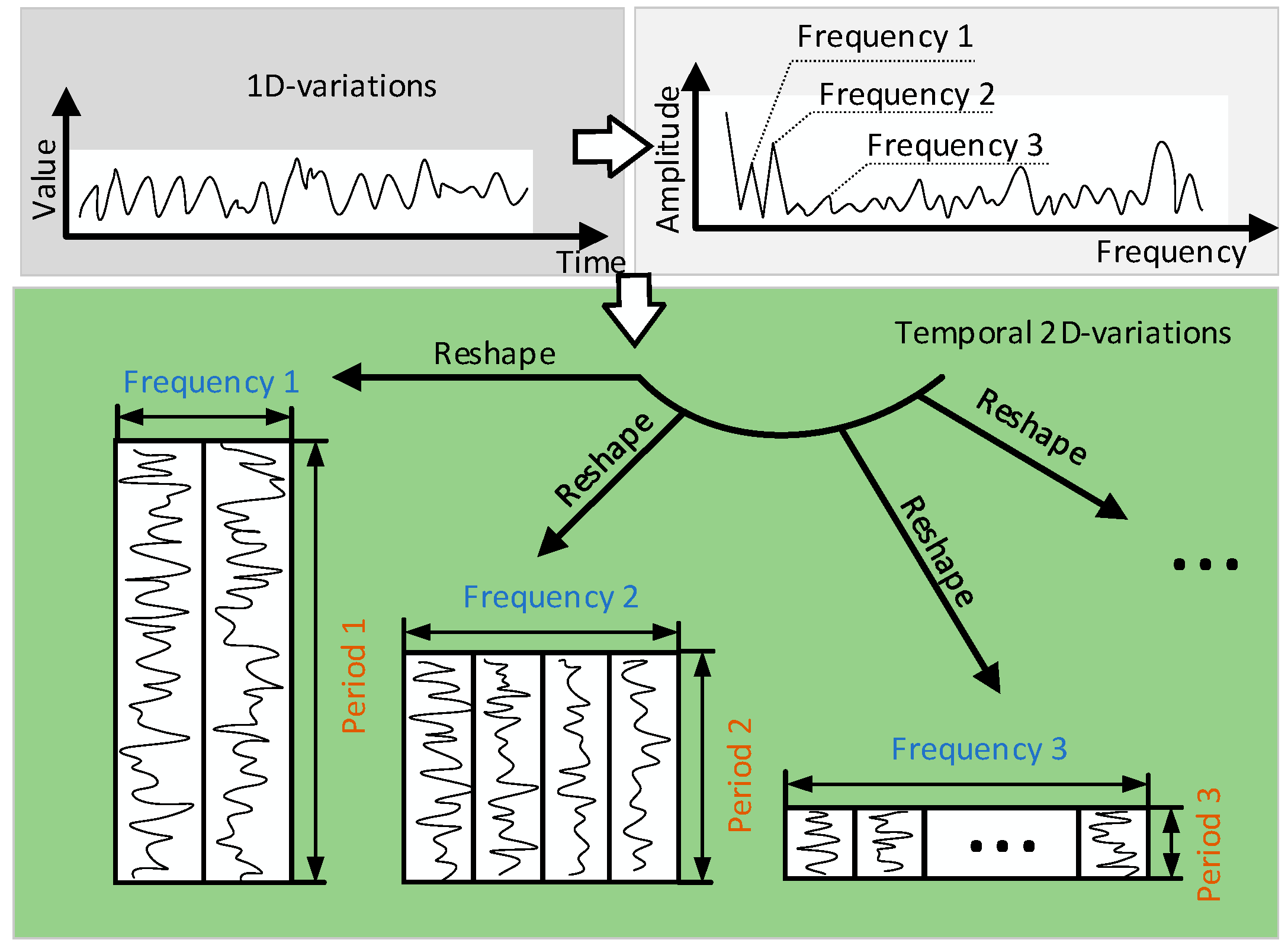
TimesNet innovatively extends one-dimensional time series data into two-dimensional space for analysis. As shown in Figure 1, collapsing a 1D time series based on multiple cycles, multiple 2D tensors can be obtained, and the columns and rows of each 2D tensor react to the temporal variations within a cycle and between cycles, respectively, to get two-dimensional (Temporal 2D variations), which decompose the complex temporal variations into different cycles through the modularized structure. The unified modeling of intra-periodic and inter-periodic variations is achieved by transforming the original one-dimensional time series into two-dimensional space.

First, for a thought time series of length T and channel dimension C: $X_{1D}\in R^{T\times C}$, its periodicity can be obtained from the Fast Fourier Transform (FFT) in the time dimension:

$$Y=Avg\left(Amp\left(FFT\left(X_{1D}\right)\right)\right),\left\{f_1,\cdots {,f}_n\right\}={}_{f_{*}\in \left\{1,\cdots ,\left[\frac{T}{2}\right]\right\}}{}^{argTopk }\left(Y\right),p_i=\left[\frac{T}{f_i}\right],i\in \left\{1,\cdots ,n\right\}$$

(1)

where $Y\in R^T$ denotes the intensity of each frequency component in $X_{1D}$ and the $n$ frequencies $\left\{f_1,\cdots f_n\right\}$ with the highest intensity corresponding to the most significant $n$ cycle lengths $\left\{p_1,\cdots p_n\right\}$. The above process can be abbreviated as:

$$Y,\left\{f_1,\cdots f_n\right\} ,\left\{p_1,\cdots p_n\right\}=Period\left(X_{1D}\right)$$

(2)

Then, the original one-dimensional time series X_1D is folded based on the selected period, which is given by the process equation:

$$X_{2D}^i={Reshape}_{p_i,f_i}\left(Padding\left(X_{1D}\right)\right),i\in \left\{1,\cdots ,n\right\}$$

(3)

where $\mathrm{P}\mathrm{a}\mathrm{d}\mathrm{d}\mathrm{i}\mathrm{n}\mathrm{g}$ denotes the addition of 0 at the end of the sequence, making the length of the sequence divisible by $p_i$. A set of two-dimensional tensors $\left\{X_{2D}^1,X_{2D}^2,\cdots ,X_{2D}^n\right\}$ can be obtained by the above operation, and $X_{2D}^i$ corresponds to the two-dimensional temporal variations dominated by the period $p_i$.

For the above 2D vectors, each column and each row correspond to a neighboring moment and a neighboring period, respectively, and the adjacent moments and periods tend to imply similar temporal variations. Therefore, the above 2D tensor will exhibit 2D localization, which makes it easy for 2D convolution to capture its information.

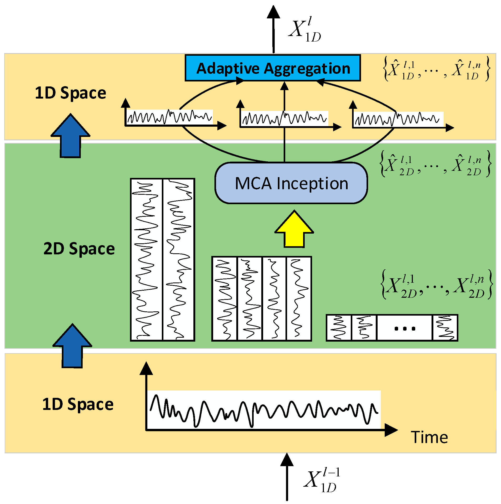
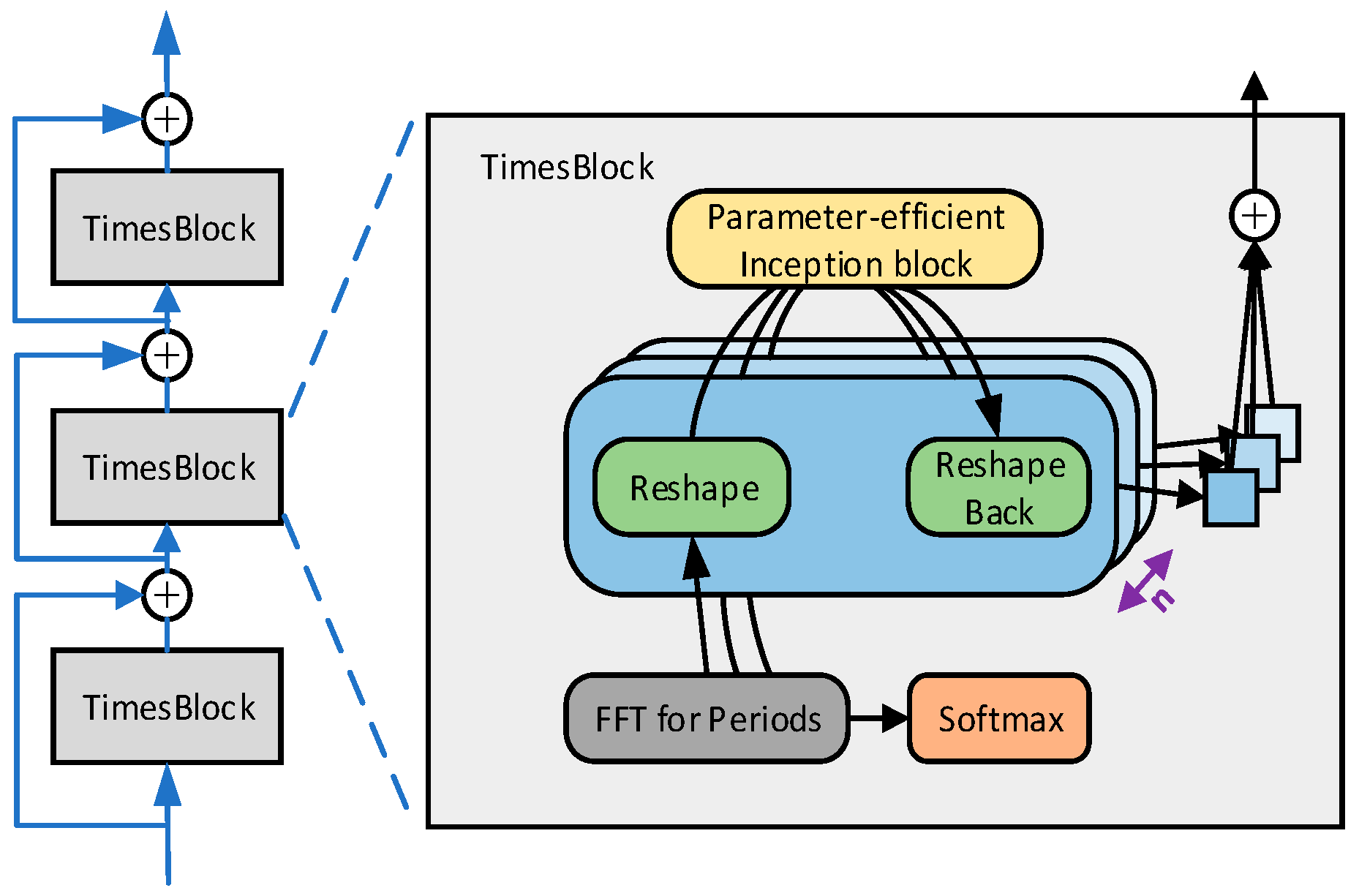
2.1.2. TimesBlock

TimesNet consists of multiple TimesBlock modules stacked using residuals, and its structure is shown in Figure 2.

The input sequence first passes through the embedding layer to obtain the depth feature $X_{1D}^0\in R^{T\times d_{model}}$. For the $l$th layer TimesBlock, the input is $X_{1D}^{l-1}\in R^{T\times d_{model}}$, after which the 2D temporal variations are extracted by 2D convolution. Its formula is:

$$X_{1D}^l=TimesBlock\left(X_{1D}^{l-1}\right)+X_{1D}^{l-1}$$

(4)

where the TimesBlock structure is shown in Figure 3 below:

It follows that a TimesBlock structure contains the following four subprocesses:

(1)

One-dimensional tensor into two-dimensional tensor: extract the input one-dimensional temporal feature $X_{1D}^{l-1}$ cycles and transform it into a two-dimensional tensor to represent the two-dimensional temporal variation, which is given by:

$$Y^{l-1},\left\{f_1,\cdots f_n\right\} ,\left\{p_1,\cdots p_n\right\}=Period\left(X_{1D}^{l-1}\right)$$

(5)

$$X_{2D}^{l,i}={Reshape}_{p_i,f_i}\left(Padding\left(X_{1D}^{l-1}\right)\right),i\in \left\{1,\cdots ,n\right\}$$

(6)

(2)

Extracting 2D time-varying features: for the 2D tensor $\left\{X_{2D}^{l,1},X_{2D}^{l,2},\cdots ,X_{2D}^{l,i}\right\}$, which has 2D localization, the information can be extracted using 2D convolution. Here, the original TimesBlock picks the classical Inception model:

$${\widehat{X}}_{2D}^{l,i}=Inception\left(X_{2D}^{l,i}\right)$$

(7)

In this paper, we add the multidimensional collaborative attention module MCA [29] to the Inception model, which is a lightweight and efficient multidimensional collective attention that utilizes a three-branch architecture to infer the channel, height, and width dimensions at the same time, with a simple and generalized structure, to be easily inserted as a plug-and-play module into a wide range of classical CNN, and to be trained in an end-to-end manner with ordinary networks, which reduces the model complexity and computational burden. The MCA structure is shown in Figure 4, so this step can be expressed as:

$${\widehat{X}}_{2D}^{l,i}=MCA\left(X_{2D}^{l,i}\right)$$

(8)

(3)

Two-dimensional tensor into one-dimensional tensor: for the extracted temporal features, they are transformed back into a one-dimensional tensor to facilitate information aggregation with the formula:

$${\widehat{X}}_{1D}^{l,i}=Teunc\left({Reshape}_{1,\left(p_i,f_i\right)}\left({\widehat{X}}_{2D}^{l,i}\right)\right),i\in \left\{1,\cdots ,n\right\}$$

(9)

where ${\widehat{X}}_{1D}^{l,i}\in R^{T\times d_{model}}$ and $\mathrm{T}\mathrm{r}\mathrm{u}\mathrm{n}\mathrm{c}$ denotes the removal of the zeros complemented by the $\mathrm{P}\mathrm{a}\mathrm{d}\mathrm{d}\mathrm{i}\mathrm{n}\mathrm{g}$ operation in step (1).

(4)

Adaptive fusion: the obtained one-dimensional tensor $\left\{{\widehat{X} }^{l,1},\cdots ,{\widehat{X} }^{l,n}\right\}$ is weighted and summed with the intensity of its corresponding frequency to obtain the final output. Its formula is:

$${\widehat{Y}}_{f_1}^{l-1},\cdots ,{\widehat{Y}}_{f_n}^{l-1}=Softmax\left(Y_{f_1}^{l-1},\cdots ,Y_{f_n}^{l-1}\right)$$

(10)

$$X_{1D}^l=\sum _{i=1}^n{\widehat{Y}}_{f_i}^{l-1}\times {\widehat{X}}_{1D}^{l,i}$$

(11)

TimesBlock can fully capture 2D-time variations at multiple scales simultaneously. Hence, TimesNet enables more efficient representation learning than directly from a one-dimensional time series.

2.2. Informer Model

The Informer model improves the Transformer model in response to the secondary computation of the Transformer model’s self-attention mechanism, the memory bottleneck of the long input stacking layer, and the speed plunge of predicting long-term outputs by (1) proposing a ProbSparse Self-attention to efficiently replace the classical Self-attention, which realizes the dependent alignment of time complexity and memory usage; (2) proposing self-attention distilling for downsampling operation, which reduces the number of dimensions and network parameters and helps to receive long sequence inputs; (3) proposing a generative decoder, which requires only one forward step to obtain long sequence outputs and at the same time avoids the inference stage of cumulative error propagation. Its overall framework is shown in Figure 5.

2.2.1. ProbSparse Self Attention

The self-attention defined in Transformer receives three inputs: query, key, and value, and then scales the dot product with the following formula:

$$A\left(Q,K,V\right)=Softmax\left(\frac{Q{K}^T}{\sqrt{d}}\right)V$$

(12)

where $Q\in R^{L_Q\times d}$, $K\in R^{L_K\times d}$, $V\in R^{L_V\times d}$, $d$ denotes the input dimension, $q_i,k_i,v_i$ denote the $i$th row of $Q, K, V$ respectively, then the attention of the $i$th query is defined as a probabilistic form of kernel smoothing method with the formula:

$$A\left(q_i,K,V\right)=\sum _j\frac{k\left(q_i,k_i\right)}{{\sum }_{l}k\left(q_i,k_i\right)}{v}_i=E_p\left(k_j|q_i\right)\left[v_j\right]$$

(13)

where $p\left(k_j|q_i\right)=\frac{k\left(q_i,k_i\right)}{{\sum }_{l}k\left(q_i,k_i\right)}$ and ${\sum }_{l}k\left(q_i,k_i\right)$ choose the asymmetric exponential kernel $exp\left(\frac{q_i{k}_j^T}{\sqrt{d}}\right)$. Self-attention weighted summation of all values by computing $p\left(k_j|q_i\right)$, a process that requires $O(L_Q L_K$) time complexity and memory usage, are the main factor that improves the predictive power.

Previous research has shown that the weights of self-attention are potentially sparse [30], and Informer investigates the sparsity of self-attention using the Kullback–Leibler scattering, where the difference between the distribution of query: $p(k_j│q_j)$, and the uniform distribution $q(k_j│q_j)$ can be measured in terms of KL dispersion:

$$KL\left(q‖p\right)=ln\sum _{l=1}^{L_K}exp(\frac{q_i{k}_j^T}{\sqrt{d}})-\frac{1}{L_K}\sum _{j=1}^{L_K}\frac{q_i{k}_j^T}{\sqrt{d}}-ln{L}_K$$

(14)

Removing the constant defines the sparsity measure of the $i$th query as:

$$M(q_i,K)=ln\sum _{l=1}^{L_K}\mathrm{e}\mathrm{x}\mathrm{p}(\frac{q_i{k}_j^T}{\sqrt{d}})-\frac{1}{L_K}\sum _{j=1}^{L_K}\frac{q_i{k}_j^T}{\sqrt{d}}$$

(15)

where the first term is the Log-Sum-Exp (LSE) operation of $q_i$ over all keys, and the second term is their arithmetic mean. If the $i$th query obtains a larger $M(q_i,K)$, it means that it has a more diverse distribution $p$ of attention weights and is likely to contain dominant dot product pairs. Therefore, for all queries, several queries with top $u$ ranked by $M(q_i,K)$ are selected as $\widehat{Q}$, where $u=cln{L}_Q$ and $c$ is a constant sampling factor, then the process of ProbSparse self-attention is represented as:

$$A\left(Q,K,V\right)=softmax\left(\frac{\widehat{Q}{K}^T}{\sqrt{d}}\right)V$$

(16)

So ProbSparse Self-attention only needs to compute $O\left(ln{L}_Q\right)$ dot products for each query-key lookup, with $O\left(L_{K}ln{L}_Q\right)$ memory usage. In the case of multiple heads, this attention generates different sparse query–key pairs for each head, thus avoiding severe information loss.

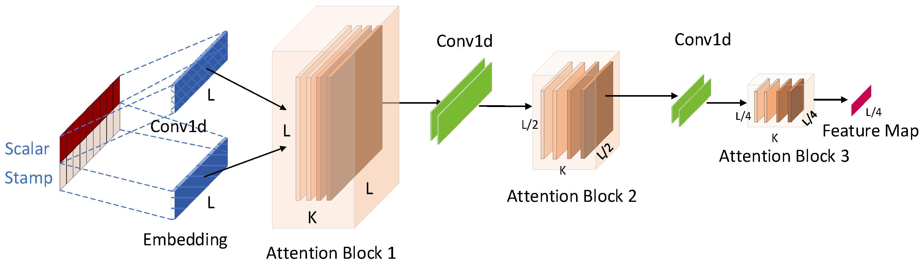
2.2.2. Encoders

The encoder is designed to allow the encoder to process longer sequence inputs by halving the individual layer features in the time dimension through an attentional distillation mechanism with limited memory, thus allowing the encoder to process longer sequence inputs, the structure of which is shown in Figure 6.

As a result of ProbSparse Self attention, there is redundancy in the feature mapping of the encoder, so the distillation operation is utilized to assign higher weights to the dominant features with dominant attention and generate focus self-attention feature mapping in the next layer. The process of distillation operation from layer $j$ to $j+1$ can be represented as:

$$X_{j+1}^t=MaxPool\left(ELU\left(Conv1d\left({\left[X_j^t\right]}_{AB}\right)\right)\right)$$

(17)

where ${\left[X_j^t\right]}_{AB}$ represents the Attention block, which contains the critical operations in the multi-head ProbSparse Self-attention and Attention block, Conv1d represents the one-dimensional convolution operation on the time series, and through ELU as the activation function, and finally, the maximum pooling operation.

Meanwhile, to enhance the robustness of the attentional distillation mechanism, the encoder carries out a halving operation of the length of the main sequence L. Each time, the length of the output sequence is half the length of the previous input sequence. After three layers of attentional blocking and two layers of convolution, a set of L/4 dimensional feature maps will be obtained, which will eventually be spliced together to form the output of the encoder.

2.2.3. Decoders

The decoder is designed to predict all the outputs of a long sequence by a single forward computation. The input data to the decoder passes through a Multi-head Masked ProbSparse Self-attention layer and a Multi-head Self-attention layer. Here, the Multi-head Masked ProbSparse Self-attention is masked to avoid autoregression. Lastly, the output dimension of the data is adjusted by the fully connected layer to get the prediction.

2.3. Attention Mechanisms

To construct a module with local and global modeling induction bias, Guangxiang Zhao et al. combined self-attention with convolution and proposed a parallel multiscale attention module called MUSE, whose structure is shown in Figure 7.

MUSE also uses an encoder–decoder framework. The encoder takes as input a sequence of word embeddings $x_1, \cdots ,x_n$, where $n$ is the length of the input. It transfers the word embeddings to a sequence of hidden representations $z_1, \cdots , z_n$. Given $z$, the decoder is responsible for generating a sequence of text $y_1,\cdots , y_m$ tokens one by one. The encoder consists of a stack of N MUSE modules. A residual mechanism and layer normalization are used to connect two adjacent layers. The decoder is similar to the encoder except that each MUSE module in the decoder captures features from the generated textual representation and performs attention on the output of the encoder stack through additional contextual attention. The critical component of the model is the MUSE module, which contains three main parts: self-attention for capturing global features, deeply separable convolution for capturing local features, and a position-level feedforward network for capturing token features. Invoking the attention mechanism in TimesNet improves the model ground feature extraction performance.

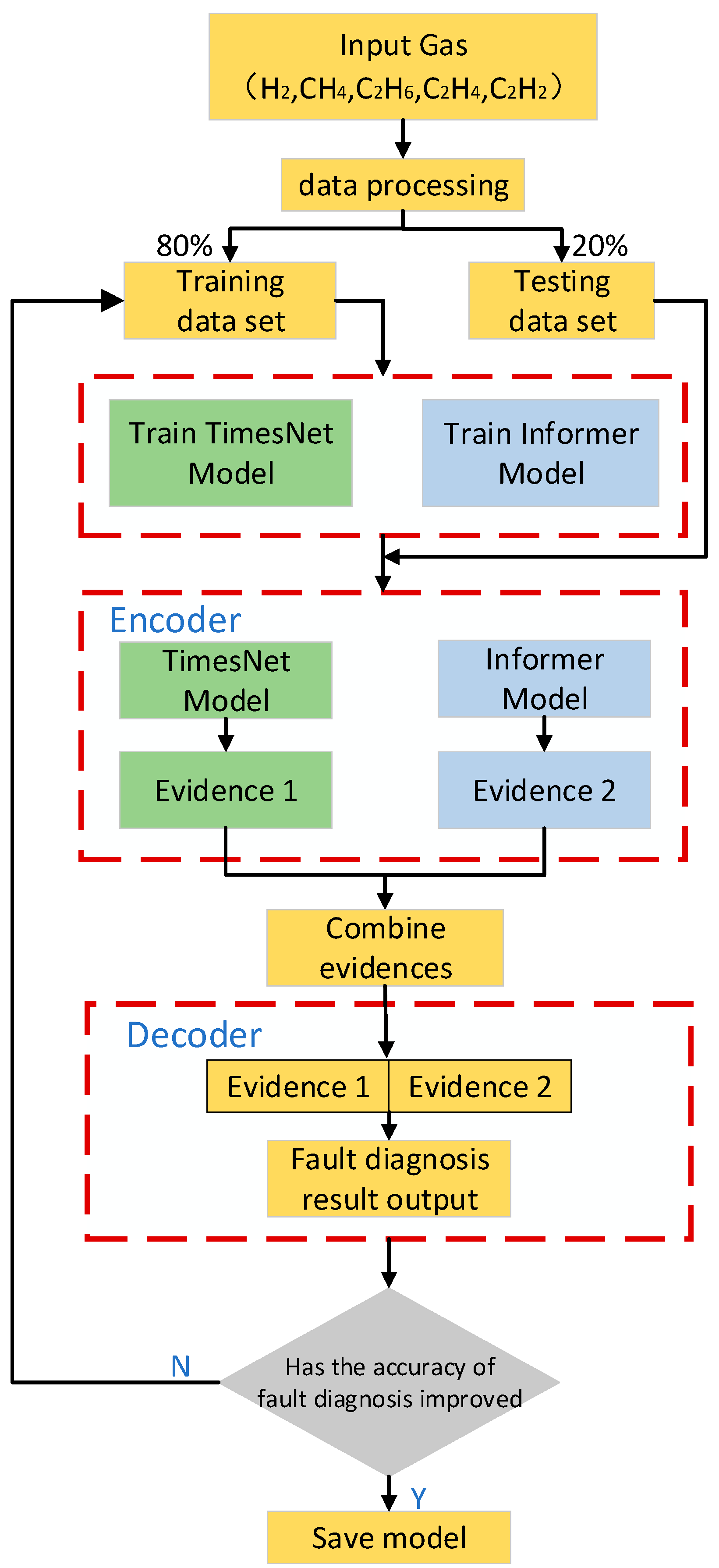
2.4. Convergence Model

To realize better transformer fault diagnosis, this paper proposes a hybrid model based on TimesNet and Informer, whose structure flow is shown in Figure 8. According to the structural flowchart of the proposed model, the detailed description of each step is as follows:

Step 1: Data processing. The transformer DGA data from the public dataset is divided into a test set and a training set in the ratio of 8:2 for learning the network model.

Step 2: Feature extraction. Feed the data into the coding layers of TimesNet and Informer respectively, TimesNet transforms the 1D time series into a set of 2D tensors based on multiple cycles, extending the analysis of temporal variations to the 2D space; TimesBlock adaptively discovers the multiple periodicities and extracts the complex temporal variations from the transformed 2D tensor; Informer uses the Transformer to construct an attention mechanism structure for sequence features and uses the global association property of the attention mechanism module for feature summarization.

Step 3: Fault diagnosis and parameter optimization. After completing the feature extraction of the transformer DGA data in the above two steps, the coding layer outputs of the two models are spliced as decoding layer inputs to obtain the final results. The model parameters are then validated using the validation set. If the model’s accuracy on the validation set is improved, the current model parameters are saved, and the model is updated for further training. Otherwise, the model parameters are modified and retrained until the best model is obtained.

3. Experiments and Analysis of Results

To evaluate the effectiveness of the proposed method, a series of experiments was conducted on the public transformer DGA dataset. To assess the model performance, a series of evaluation metrics was selected, including Precision, Recall, Accuracy, and F1, which are defined as:

$$Precision=\frac{TP}{TP+FP}$$

(18)

$$Recall=\frac{TP}{TP+FN}$$

(19)

$$Accuracy=\frac{TP+TN}{TP+TN+FP+FN}$$

(20)

$$F_1=\frac{2·Precision·Recall}{Precision+Recall}$$

(21)

where TP is true positive, i.e., the number of positive samples identified as positive; FP is false positive, i.e., the number of negative samples identified as positive; TN is true negative, i.e., the number of negative samples identified as unfavorable; and FN is false negative, i.e., the number of positive samples identified as hostile.

In addition, to highlight the advantages of the proposed method, this paper compares it with a single model such as Transformer and Informer.

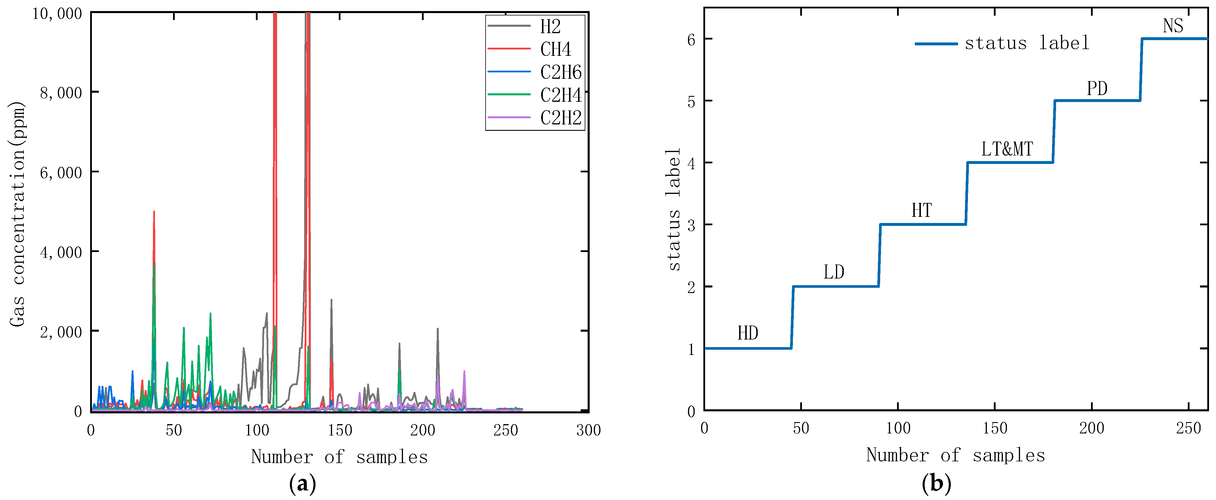
3.1. Data Preparation

In this paper, 260 publicly available transformer DGA datasets were collected. The gas contents used in five commonly used dissolved gas analysis methods in oil, namely H₂, CH₄, C₂H₆, C₂H₄, and C₂H₂, were adopted as the criteria for fault diagnosis. The data were classified into six categories according to the type of faults [31], namely, high-energy discharge (HD), low-energy discharge (LD), high-temperature overheating (HT), low and medium temperature overheating (LT&MT), partial discharge (PD), and normal (NS) six classifications, and the data were divided into the training set and test set in the ratio of 8:2. The five gas concentrations and their state labels for each sample are shown in Figure 9. The details of the training and test set samples are shown in

Table 1. Sample distribution of the first dataset.

Fault Type	Serial Number	Total Number of Samples	The Sample Size of the Training Set	The Sample Size of the Testing Set
high-energy discharge	HD	45	36	9
low-energy discharge	LD	45	36	9
high-temperature overheating	HT	45	36	9
Low- and medium-temperature overheating	LT&MT	45	36	9
partial discharge	PD	45	36	9
normal	NS	35	28	7

.

3.2. Experimental Environment and Parameter Settings

This experiment uses Pytorch deep learning framework, the hardware environment CPU is 12th Gen Intel(R) Core(TM) i7-12700H 2.30 Hz, GPU is NVIDIA GeForce PTX 3060 Laptop, the operating system is Windows 11, and Python version is 3.7.

To ensure the accuracy of the experimental results, the model parameters in the comparison experiments are set as follows: batch_size is 16, the optimizer is Adam, the learning rate is 0.001, the loss function is the cross-entropy loss function CrossEntropyLoss, the training epoch is 20, and at the same time, the patience is set to 10 and the training is ended when the network is trained for 10 rounds and there is still no effect improvement.

3.3. Ablation Experiments

For the different improvement methods: the MCA-TimesNet model formed by introducing the MCA module into the Inception structure of the original TimsesNet; the MUSE-TimesNet model after the introduction of the MUSE Attention Mechanism; the hybrid model that fuses TimsesNet with Informer; and the improved hybrid model that combines TimsesNet with Informer are tested and trained on the DGA dataset to get the fault diagnostic performances of the models after the different improvement methods, and the results are shown in

Table 2. Performance comparison of different improved methods.

Models	Precision	Recall	Accuracy	F1
TimesNet	83.45%	80.95%	93.55%	80.18%
MCA-TimesNet	84.15%	83.3%	94.22%	81.72%
MUSE-TimesNet	86%	85.2%	94.85%	84.18%
Hybrid model	87.9%	87.05%	95.51%	86.18%
Methodology of this paper	89.52%	88.9%	96.15%	88.4%

.

The positive impact of each improvement method on the model can be observed through ablation experiments. After introducing the MCA module into the original TimesNet’s Inception model, the accuracy improved to 94.22%; after introducing the MUSE attention mechanism, the accuracy improved to 94.85%; after fusing TimesNet with the Informer model, the accuracy improved to 95.51%; after combining the MCA and the MUSE-improved TimesNet connected with the Informer model, the accuracy is the highest at 96.15%. All other performances are also improved to different degrees, which shows that the method proposed in this paper has advantages in transformer fault diagnosis.

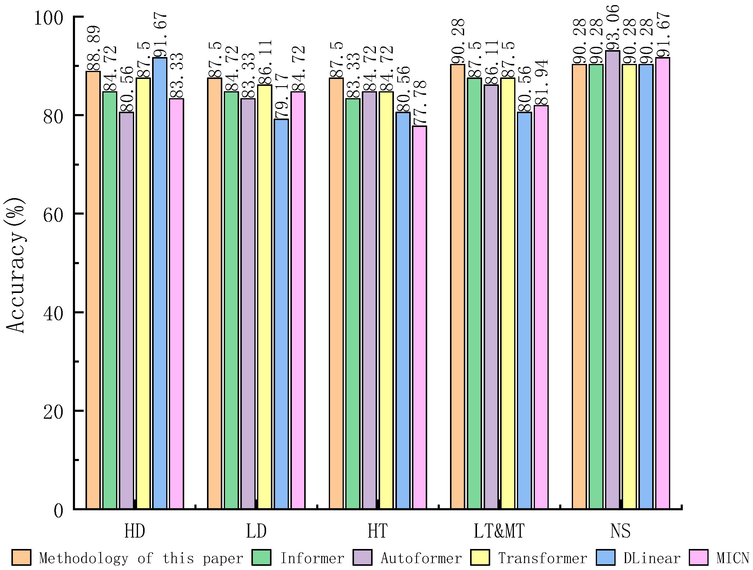
3.4. Comparative Experiments

To prove that the multi-model fusion method proposed in this paper is more advantageous than the single model, the model of this paper is compared with the classical models, such as Informer and Transformer, under the same experimental conditions, and the performance of different models is shown in

Table 3. Performance comparison of different models.

Models	Precision	Recall	Accuracy	F1
Methodology of this paper	89.52%	88.89%	96.15%	88.41%
Informer	84.49%	77.52%	92.95%	77.63%
Autoformer	79.56%	75.39%	91.67%	73.97%
Transformer	81.26%	76.19%	92.31%	76.16%
DLinear	50.59%	61.11%	87.82%	52.99%
MICN	40.82%	41.27%	80.77%	33.96%

. The recognition ability of this paper’s method and single model for each fault type is shown in

Table 4. Diagnostic accuracy of each model for different types of faults.

	Methodology of This Paper	Informer	Autoformer	Transformer	DLinear	MICN
HD	96.15%	88.46%	90.38%	92.31%	92.31%	75%
LD	100%	100%	100%	100%	100%	82.69%
HT	94.23%	88.46%	82.69%	84.62%	69.23%	69.23%
LT&MT	92.31%	90.38%	84.62%	88.46%	82.69%	82.69%
PD	96.15%	98.07%	96.15%	96.15%	96.15%	88.46%
NS	98.07%	92.31%	96.15%	92.31%	86.53%	86.53%
average	96.15%	92.95%	91.67%	92.31%	87.82%	80.77%

.

As can be seen from Table 3, this paper’s method performs well in all indicators, and all indicators are best compared to the single model. Precision, Recall, Accuracy, and F1 indicators reach 89.52%, 88.89%, 96.15%, and 88.41%, respectively, higher than those of Informer and Autoformer, Transformer, and other single models.

From Table 4, it can be seen that the method of this paper has the best diagnostic effect on HD; except for MICN, the diagnostic impact of each model on LD reaches 100%; for HT, the method of this paper has the best effect; for LT&MT, the proposed method of this paper has the best result; for PD, Informer has the best effect; and for NS, the result of this paper has the best result. Overall, compared to a single model, the method in this paper provides the best fault diagnosis results, and the accuracy is improved by 3.21%, 4.48%, 4.07%, 8.33%, and 15.38% compared to Informer, Autoformer, Transformer, DLinear, and MICN, respectively. This proves the advantages of the multi-model fusion method proposed in this paper.

Figure 10 shows the fault diagnosis results of each method on the test set, where the blue circle indicates the actual fault type of the sample, the red plus sign indicates the fault type recognized by the method, and the two marking point types overlap, showing the diagnosis results of the fault. From the figure, it can be seen that for 52 sets of test set data, the method of this paper identifies the most number of correct ones, 46 groups, with a proper rate of 88.46%; Informer is the number of correct ones, 41 groups, with an appropriate rate of 78.85%; Autoformer identifies the number of correct ones, 39 groups, with a proper rate of 75%; and Transformer recognizes the correct ones, 40 groups, with an appropriate rate of 76.85%; and the number of correct ones, 40 groups, with a proper rate of 75%. Forty groups with an applicable rate of 76.92%; DLinear recognizes the valid number of 33 groups with a correct rate of 63.46%; and MICN identifies the right number of 22 groups with a proper rate of 42.31%. From the fault diagnosis results of this paper’s method, it can be seen that it has the highest correct rate of identifying LD, HT, and NS, and the samples of these three faults are accurately identified. In contrast, although the method is not very effective in identifying HD and LT&MT, it has reached a high level. Figure 10 shows that this paper’s method can generally recognize transformer faults with high accuracy, and the accuracy is significantly improved compared to a single model.

The confusion matrix is a situation analysis table in machine learning that summarizes the prediction results of classification models in the form of a matrix that summarizes the records in the dataset according to two criteria: the proper categories and the category judgments predicted by the classification models, and Figure 11 shows the confusion matrices for each method.

By comparing the confusion matrices, it can be seen that different models have different recognition abilities for various faults. It is worth mentioning that, except for MICN, these models have excellent recognition abilities for LD. Still, some models have poor recognition abilities for specific faults, such as DLinear’s recognition of LT&MT and NS and MICN’s recognition of LD. Informer’s recognition of NS is relatively poor, and Autoformer’s recognition of LT&MT is poor. Informer’s recognition of NS is poor, and Autoformer’s recognition of LT&MT is poor. In contrast, the recognition ability of the method proposed in this paper for each type of fault reaches a high level, further proving the advantage of the technique offered in transformer fault diagnosis.

3.5. Experimental Results for Different Datasets

To verify the performance of the proposed method on different DGA datasets, the proposed method is experimentally validated on another publicly available 350-group DGA dataset. Unlike the previous dataset, the distribution of faults in this dataset is more uneven. The fault types are different from the previous one, which are divided into five types: high-energy discharge (HD), low-energy discharge (LD), high-temperature overheating (HT), medium-low-temperature overheating (LT&MT), and normal (NS), which are also divided into the training set and the test set in the ratio of 8:2. This dataset is more complex and better reflects the actual situation of transformer failure during operation. Its data division is shown in

Table 5. Sample distribution of the second dataset.

Fault Type	Serial Number	Total Number of Samples	The Sample Size of the Training Set	The Sample Size of the Testing Set
high-energy discharge	HD	95	76	19
low-energy discharge	LD	58	46	12
high-temperature overheating	HT	109	87	22
low and medium-temperature overheating	LT&MT	56	44	12
normal	NS	37	30	7

. In this experiment, the models were evaluated under the same conditions, and their results are shown in

Table 6. Performance comparison of different methods.

Models	Precision	Recall	Accuracy	F1
Methodology of this paper	68.94%	65.26%	88.89%	66.32%
Informer	61.93%	58.24%	86.11%	58.3%
Autoformer	67.55%	54.97%	85.56%	53.54%
Transformer	64.68%	61.02%	87.22%	61.41%
DLinear	49.93%	54.13%	84.45%	50.46%
MICN	56.81%	50.88%	83.89%	50.34%

. Figure 12 shows the recognition accuracy of different models for each fault.

As shown in Table 6, the fault diagnosis performance of each model has decreased compared to the previous dataset, which is due to the uneven distribution of the dataset, which makes the feature extraction of the model for faults complicated. In contrast, the proposed method’s Precision, Recall, Accuracy, and F1 values on this dataset still outperform the other single models. The diagnostic accuracy of each model for different faults can be seen in Figure 12. The diagnostic accuracy of this paper’s method for LD, HT, and LT&MT is still the highest, and the diagnostic accuracy for HD and NS is not optimal. Still, it is also at a high level, and the experimental results once again proved this paper’s method’s applicability on different datasets, indicating that it is advantageous for diagnosing transformer faults.

4. Conclusions

In this paper, a multi-model fusion transformer fault diagnosis method based on TimesNet and Informer is proposed to improve the original TimesNet as follows:

(1)

Introducing the Multidimensional Collaborative Attention Module MCA into the Inception structure of TimesBlock reduces the model complexity and the computational burden.

(2)

The MUSE attention mechanism in TimesNet was introduced to improve the feature extraction capability of the model for transformer faults.

(3)

The TimesNet and Informer multilayer parallel feature extraction modules are introduced in the construction of the feature module, making full use of the local features of the convolution and the global correlation of the attention mechanism module for feature aggregation, which can effectively extract the correlation characteristics of the time-series data within the cycle and between the cycles, as well as constructing the correlation information among the different local features for the long sequences, to allow the model to learn more time-series information to enhance its effectiveness in fault diagnosis.

Ablation experiments and comparison experiments on the public DGA dataset can lead to the following conclusions:

(1)

All the different improvement methods positively affect the original TimesNet model, and the accuracy of the MCA-TimesNet model reaches 94.22%; the accuracy of the MUSE-TimesNet model reaches 94.85%; and the accuracy of the Hybrid model reaches 95.51%; the method in this paper combines the three improvement methods, and the final accuracy reaches 96.15%.

(2)

The fusion model of TimesNet and Informer proposed in this paper is more effective in transformer fault diagnosis and has a more extraordinary vital fault identification ability. The accuracy rate is improved by 3.21%, 4.48%, 4.07%, 8.33%, and 15.38%, respectively, compared with the single models of Informer, Autoformer, Transformer, DLinear, and MICN.

(3)

On different data sets, the fault recognition ability of the method proposed in this paper is also high, with an accuracy rate of 88.89%, which is highly applicable and can provide a reference for transformer fault diagnosis.