Distributed Coordination $\mathcal{D}$-Stabilization in Cyclic Pursuit Formations of Dynamical Multi-Agent Systems ^†

Abstract

In this study, the cyclic pursuit formation stabilization problem in target-enclosing operations by multiple homogeneous dynamic agents is investigated. To this end, a Lyapunov $\mathcal{D}$-stability problem is first formulated to cover the transient performance requirements for multi-agent systems. Then, a simple diagrammatic Lyapunov $\mathcal{D}$-stability criterion for cyclic pursuit formation is derived. The formation control scheme combined with a cyclic-pursuit-based distributed online path generator satisfying this condition guarantees both the required transient performance and global convergence properties with theoretical rigor. It is shown that the maximization of the connectivity gain in a cyclic-pursuit-based online path generator can be reduced to an optimization problem subject to linear matrix inequality constraints derived using the generalized Kalman-Yakubovich–Popov lemma. This approach provides a permissible range of connectivity gain, which not only guarantees global formation stability/convergence properties but also satisfies the required performance specification. Several numerical examples are provided to confirm the effectiveness of the proposed method.

1. Introduction

Formation control, which coordinates the motion of relatively simple and inexpensive multiple agents, is increasingly essential for expanding operational areas and executing complex tasks in diverse fields such as surveillance, search and rescue, and environmental monitoring (see [1,2,3] and the references therein). The use of multi-agent systems (MAS) has emerged as a robust solution, which are particularly advantageous in scenarios that involve hazardous missions where the potential for agent loss is high. These systems deploy multiple lower-performance agents, as opposed to a single high-performance agent, enabling them to handle complex operations that are typically unmanageable for individual agents.

Recent advancements in formation control are especially significant in aerospace applications, including unmanned aerial vehicles (UAVs) and satellites, where strategic formations drastically improve observational capabilities and operational interventions [4,5]. Amid these developments, several research groups have focused on coordination control strategies that allow for an enclosing formation around specific areas or objects using local information [6,7,8,9,10,11,12,13,14,15,16,17]. This approach enhances the effectiveness of surveillance and task-oriented missions by ensuring agents operate within a defined spatial domain, thereby maximizing coverage and responsiveness. Enclosing formations, often achieved through techniques like cyclic pursuit, are pivotal in scenarios where minimal communication and high resilience to system dynamics are required. Cyclic pursuit, known for its minimal communication requirements and resilience to dynamic group changes, has been identified as an effective formation control strategy [6,9]. This approach only necessitates the relative positions of neighboring agents, thereby reducing the communication load and increasing adaptability to interference and alterations within the group. Continuing research has focused on enhancing cyclic pursuit strategies for dynamic target tracking [8,10,12,13], adapting formation geometries to track multiple targets simultaneously [14,15,16,18], and developing innovative methods that apply cyclic pursuit to practical, real-world scenarios [4,9,19]. These explorations pave the way for innovative applications of cyclic pursuit, such as the approach proposed by Kim and Sugie [20], which further refines path-planning methodologies for target-enclosing operations.

In this line of research, Kim and Sugie [20] proposed a distributed online path-planning method for target-enclosing operations by multi-agent systems based on a modified cyclic pursuit strategy. However, despite its simple but particularly effective nature for target-enclosing tasks, the aforementioned method could present a critical drawback in real implementations where each agent is assumed to be a point mass with full actuation. In particular, ignoring the agent’s dynamics may cause a potential problem where each agent cannot precisely track its designed trajectory or the global convergence of multiple agents, meaning that the designated formation may not be achieved. To overcome the above-mentioned difficulties, Kwak et al. [21] and Kim et al. [22] developed simple diagrammatic Lyapunov and asymptotic formation stability criteria, which are the significant extension of a stability analysis method for linear systems with a generalized frequency variable proposed in [23,24] and investigated in [25]. The formation control scheme combined with a cyclic-pursuit-based distributed online path generator satisfying those stability criteria guarantees the required global convergence properties with theoretical rigor.

In this paper, multiple agents in three-dimensional (3D) space are considered, with homogeneous system dynamics locally controlled by identical controllers. For such multi-agent dynamical systems, a new optimization-based formation stabilization strategy for cyclic pursuit-based distributed cooperative control in target-enclosing operations is proposed. To this end, a Lyapunov $\mathcal{D}$-stability problem, which covers the requirements for the transient performance of multi-agent dynamical systems, is first formulated in Section 3.1. Then, a simple diagrammatic Lyapunov $\mathcal{D}$-stability criterion for cyclic pursuit formation is developed in Section 3.2. The formation control scheme, combined with a cyclic pursuit-based distributed online path generator satisfying this condition, guarantees both the required transient performance and global convergence properties with theoretical rigor. The following optimization problem for pursuit formation stabilization is considered on the basis of the above results:

[Problem S] Maximization of a connectivity gain in a cyclic pursuit-based online path generator, which satisfies, for a given agent’s dynamics and its local controller, not only a global formation stability condition but also the required transient performance specifications.

To derive an optimization problem for “Problem S”, it is first shown in Section 4 that the required pursuit formation $\mathcal{D}$-stability condition can be converted into a linear matrix inequality (LMI) optimization problem that is numerically tractable and can be solved efficiently, utilizing the generalized Kalman–Yakubovich–Popov (GKYP) lemma [26,27]. A concrete optimization problem subject to LMI constraint conditions for maximizing the connectivity gain, which satisfies the requirements mentioned in “Problem S”, is developed. Several numerical examples are provided in Section 5 to illustrate its distinctive features and the achievement of the desired pursuit pattern.

The main contributions of this study are as follows:

• Introduction of Lyapunov $\mathcal{D}$-stabilization for cyclic-pursuit-based multi-agent systems:
  This study pioneers the incorporation of Lyapunov $\mathcal{D}$-stabilization techniques within cyclic-pursuit-based multi-agent systems. The $\mathcal{D}$-stabilization approach is designed to ensure desirable transient responses and convergence to stable formations in multi-agent systems. By employing the GKYP lemma, the proposed framework systematically guarantees stability and robustness under diverse conditions, providing a rigorous theoretical foundation.
• Scalable optimization approach for large-scale systems:
  A novel LMI-based optimization method is proposed, offering a significant computational advantage by ensuring that the complexity of stability analysis is independent of the number of agents in the system. Unlike traditional methods that rely on collective system dynamics and incur computational costs proportional to system size, the proposed method focuses exclusively on individual agent dynamics. This modular design enables the optimization problem to maintain a fixed dimensionality, making it highly scalable and efficient for large-scale systems. Moreover, the independence from global system dynamics enhances its feasibility for distributed or decentralized control architectures, which are crucial for real-world multi-agent applications.
• Validation through diverse numerical experiments:
  The proposed framework is validated through a series of numerical experiments encompassing both high-order and low-order agent dynamics. These experiments illustrate the effectiveness of the $\mathcal{D}$-stabilization framework under various operating conditions and demonstrate its adaptability to different system complexities. The results emphasize the practicality and versatility of the framework in achieving robust and stable formations in multi-agent systems.

Additionally, this study addresses critical issues identified in earlier work [28], authored in part by one of the co-investigators of this paper. The prior research faced significant challenges in formulating an optimization framework for determining the maximum connectivity gain, which resulted in incomplete and inaccurate stability analysis. This study not only corrects those errors but also provides a robust optimization methodology that systematically guarantees the desired stability and transient performance in multi-agent systems. By resolving these limitations, the proposed approach ensures a theoretically rigorous and practically applicable solution for distributed coordination stabilization.

Notations: For a Hermitian matrix, $M>0$, $M\ge 0$, $M<0$, and $M\le 0$ denote positive definiteness, positive semidefiniteness, negative definiteness, and negative semidefiniteness, respectively. The transpose and complex-conjugate transpose of the matrix M are denoted by $M^T$ and $M^{*}$, respectively. The symbol ${\mathbf{H}}_n$ denotes the set of $n\times n$ Hermitian matrices. The Kronecker product of matrices $\mathsf{\Gamma }$ and P is $\mathsf{\Gamma }\otimes P$. The real and imaginary parts of a complex variable z are represented by $\mathrm{Re}\left[z\right]$ and $\mathrm{Im}\left[z\right]$, respectively.

2. System Description and Control Aim

2.1. System Description

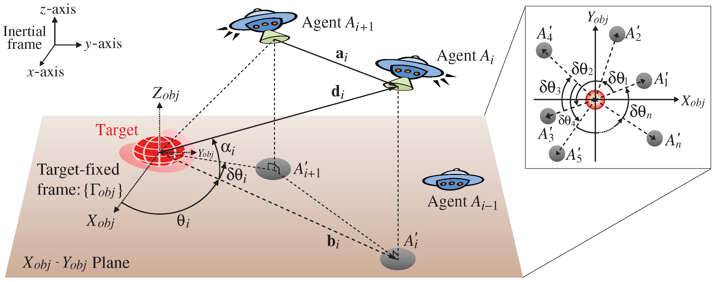
In this study, the same multi-agent dynamical system as the one investigated in [21,22] is considered; specifically, a group of n agents dispersed in 3D space, as shown in Figure 1. All agents are ordered from 1 to n, i.e., $A_1,A_2,\cdots ,A_n$. The agent $A_{i+1}$ is defined as the prey agent of $A_i$ (In what follows, the subscript “$n+1$” is equivalent to “1”; that is, the case in which the i-th agent simply pursues the ($i+1$)-th agent with modulo n is considered). Denote the position vectors of the stationary target object and moving agent $A_i$ ($i=1,2,\cdots ,n$) in the inertial frame as ${\mathit{x}}_o\in {\mathbb{R}}^3$ and ${\mathit{x}}_i\left(t\right)\in {\mathbb{R}}^3$, respectively. It is assumed that the i-th agent $A_i$ can measure ${\mathbf{d}}_i:={\mathit{x}}_i-{\mathit{x}}_o$ and ${\mathbf{a}}_i:={\mathit{x}}_i-{\mathit{x}}_{i+1}$. Define the target-fixed frame $\left\{{\mathsf{\Gamma }}_{obj}\right\}$ in which the origin is at the center of the target object and $X_{obj}$-, $Y_{obj}$-, and $Z_{obj}$-axes are respectively parallel to the x-, y-, and z-axes of the inertial frame. Let ${\mathbf{b}}_i$ denote the vector of ${\mathbf{d}}_i$ projected onto the $X_{obj}$-$Y_{obj}$ plane in the target-fixed frame and define three scalars: ${\theta }_i=\angle ({\mathbf{e}}_x,{\mathbf{b}}_i)$, ${\alpha }_i=\angle ({\mathbf{b}}_i,{\mathbf{d}}_i)$, and $d_i:=\left|{\mathbf{d}}_i\right|$, where ${\mathbf{e}}_x$ denotes the unit vector in the $X_{obj}$-direction of $\left\{{\mathsf{\Gamma }}_{obj}\right\}$, and $\angle (\mathbf{x},\mathbf{y})$ denotes the counterclockwise angle from the vector $\mathbf{x}$ to the vector $\mathbf{y}$. Then, ${\mathbf{d}}_i$ can be represented as ${\mathbf{d}}_i={[d_{i}cos{\theta }_{i}cos{\alpha }_i,d_{i}sin{\theta }_{i}cos{\alpha }_i,d_{i}sin{\alpha }_i]}^T$. The variables ${\theta }_{i+1}$ and $\delta {\theta }_i$($:={\theta }_{i+1}-{\theta }_i$) can be calculated in a similar way because ${\mathbf{d}}_{i+1}={\mathbf{d}}_i-{\mathbf{a}}_i$ holds. Here, $\delta {\theta }_i$ represents the angular difference between consecutive agents.

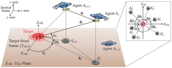
Figure 1. System description.

Suppose that all agents $A_i$ ($i=1,2,\cdots ,n$) have common system dynamics described by a multiple-input, multiple-output (MIMO) plant:

$${\mathbf{y}}_i\left(s\right):={[{\theta }_i\left(s\right),d_i\left(s\right),{\alpha }_i\left(s\right)]}^T=\mathbf{P}\left(s\right){\mathbf{u}}_i\left(s\right),$$

(1)

where ${\mathbf{y}}_i\left(s\right)$ is the system output, ${\mathbf{u}}_i\left(s\right)$ is the control input, and $\mathbf{P}\left(s\right)$ is a diagonal transfer matrix expressed as

$$\mathbf{P}\left(s\right):=\mathrm{diag}(p_{\theta }\left(s\right),p_d\left(s\right),p_{\alpha }\left(s\right)).$$

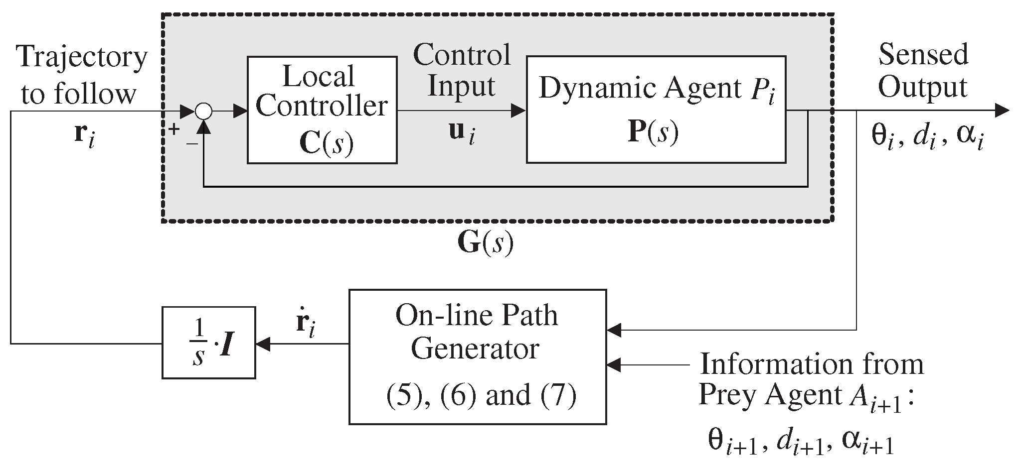
Furthermore, assume that all agents are asymptotically stabilized by an identical local diagonal feedback controller $\mathbf{C}\left(s\right)$ defined by

$$\mathbf{C}\left(s\right):=\mathrm{diag}(c_{\theta }\left(s\right),c_d\left(s\right),c_{\alpha }\left(s\right)),$$

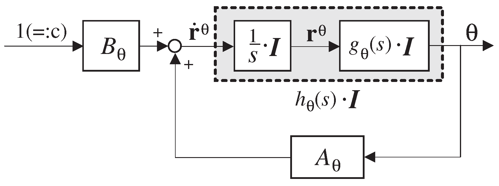
as illustrated in Figure 2. Then, the $\theta$-, d-, and $\alpha$-directional closed-loop transfer functions of agent $A_i$ are respectively described as follows:

$$\begin{array}{cc}\hfill & g_{\theta }\left(s\right)={\displaystyle \frac{p_{\theta }\left(s\right)c_{\theta }\left(s\right)}{1+p_{\theta }\left(s\right)c_{\theta }\left(s\right)}},\hfill \end{array}$$

(2)

$$\begin{array}{cc}\hfill & g_d\left(s\right)={\displaystyle \frac{p_d\left(s\right)c_d\left(s\right)}{1+p_d\left(s\right)c_d\left(s\right)}},\hfill \end{array}$$

(3)

$$\begin{array}{cc}\hfill & g_{\alpha }\left(s\right)={\displaystyle \frac{p_{\alpha }\left(s\right)c_{\alpha }\left(s\right)}{1+p_{\alpha }\left(s\right)c_{\alpha }\left(s\right)}}.\hfill \end{array}$$

(4)

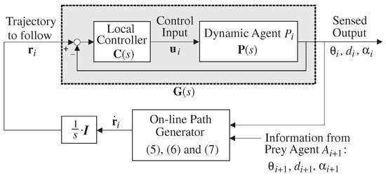
Figure 2. Formation controller configuration.

Now, the procedure of forming the following geometric pattern for a target-enclosing operation by n dynamic agents is considered:

(A1) $\delta {\theta }_i\left(t\right)\to 2\pi /n$[rad] as $t\to \infty$ (i.e., n agents enclose the target object at a uniformly spaced angle and maintain this angle),

(A2) $d_i\left(t\right)\to D$ as $t\to \infty$ (i.e., each agent approaches the target object and finally keeps a distance D),

(A3) ${\alpha }_i\left(t\right)\to \mathsf{\Phi }$[rad] as $t\to \infty$ (i.e., the angle ${\alpha }_i$, which corresponds to the altitude of each agent, converges to the desired one, $\mathsf{\Phi }$),

• where D and $\mathsf{\Phi }$ are given by the designer (For the sake of clarity, this paper only considers the equal convergence positions for all dynamic agents; i.e., $D_1=D_2=\cdots =D_n=D$ and ${\mathsf{\Phi }}_1={\mathsf{\Phi }}_2=\cdots ={\mathsf{\Phi }}_n=\mathsf{\Phi }$, while the distinct ones for each agent can be assigned). Here, the following distributed online path-planning scheme for the ith agent $A_i$ is introduced [20]:

  $$\begin{array}{cc}\hfill & {\dot{r}}_i^{\theta }\left(t\right)=k_{\theta }\delta {\theta }_i\left(t\right),\hfill \end{array}$$

  (5)

  $$\begin{array}{cc}\hfill & {\dot{r}}_i^d\left(t\right)=k_d(D-d_i\left(t\right)),\hfill \end{array}$$

  (6)

  $$\begin{array}{cc}\hfill & {\dot{r}}_i^{\alpha }\left(t\right)=k_{\alpha }(\mathsf{\Phi }-{\alpha }_i\left(t\right)),\hfill \end{array}$$

  (7)

  where $k_{\theta }$, $k_d$, and $k_{\alpha }$ ($>0$) are design parameters, and $\delta {\theta }_i\left(t\right)$ is defined as follows:

  $$\left\{\begin{array}{cc}\delta {\theta }_i\left(t\right):={\theta }_{i+1}\left(t\right)-{\theta }_i\left(t\right),\hfill & i=1,2,\cdots ,n-1\hfill \\ \delta {\theta }_n\left(t\right):={\theta }_1\left(t\right)-{\theta }_n\left(t\right)+2\pi ,\hfill & i=n.\hfill \end{array}\right.$$

  The reference position ${\mathbf{r}}_i\left(t\right)={[r_i^{\theta }\left(t\right),r_i^d\left(t\right),r_i^{\alpha }\left(t\right)]}^T$ shown in Figure 2 is designed by using (5)–(7).

2.2. Control Aim with a Motivating Example

For a cooperative target-enclosing formation by multiple homogeneous dynamic agents described in Section 2.1, some studies [21,22] have provided a considerably simple diagrammatic Lyapunov/asymptotic stability analysis scheme. Their results suggest the process to determine $k_{\theta }$, $k_d$, and $k_{\alpha }$ in (5)–(7) to guarantee that all agents assemble in the desired formation around the target object in 3D space (see Theorems 5.1 and 5.2 in [22]). Nevertheless, no explicit information about the transient performance of formation control laws is obtained from their scheme in a direct manner, which is illustrated in the following example.

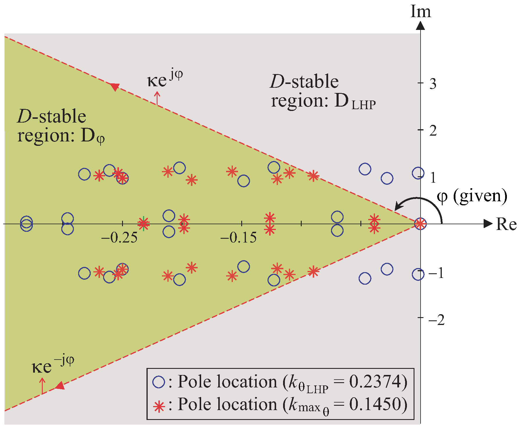
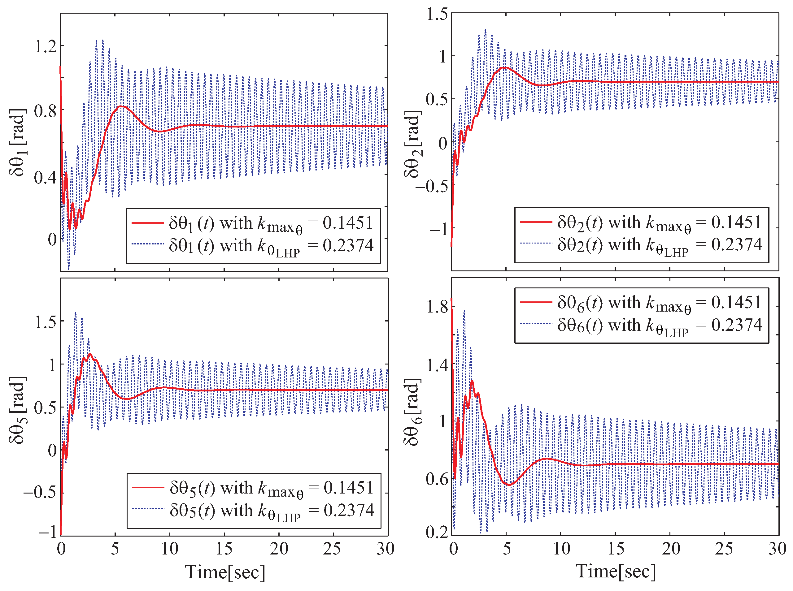
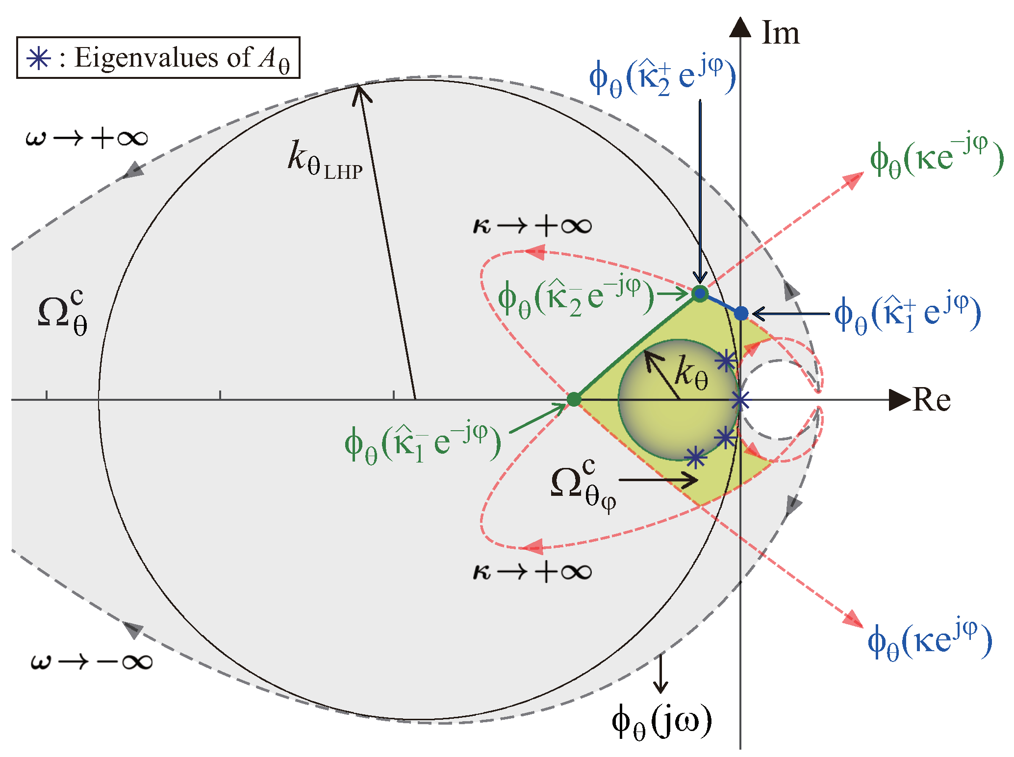
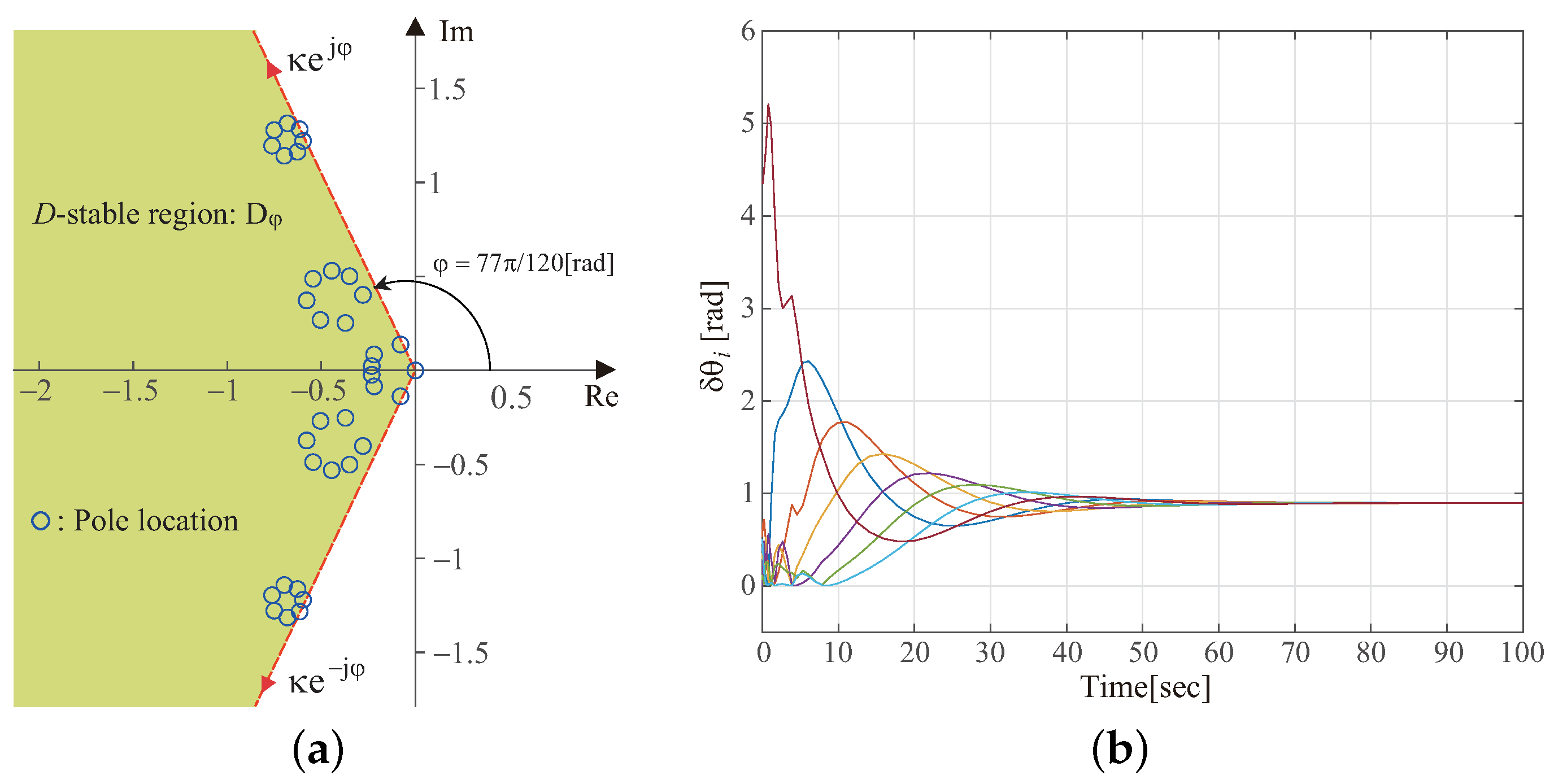
Suppose that $n=8$ agents have common dynamics $p_{\theta }\left(s\right)=1/s(s-0.5)$ and its stabilizing local proportional-derivative (PD) controller is given as $c_{\theta }\left(s\right)=1+s$. Here, $k_{\theta }$ in (5) is set as $k_{\theta }=0.2374(=:k_{{\theta }_{\mathrm{LHP}}})$, which satisfies the Lyapunov stability condition given in [22] and thus enables all nonzero poles of ${\mathcal{H}}_{\theta }\left(s\right)$ to be located in the left-half complex plane (${\mathrm{D}}_{\mathrm{LHP}}$) as shown in Figure 3. In this case, some of the time responses of $\delta {\theta }_i\left(t\right)$ ($i=1,2,5,6$) are illustrated using dotted lines in Figure 4. Figure 4 reveals that the choice of $k_{\theta }=k_{{\theta }_{\mathrm{LHP}}}$ guarantees that ${lim}_{t\to \infty }\delta {\theta }_i\left(t\right)\to 2\pi /8\left[\mathrm{rad}\right]$ ($i=1,2,\cdots ,8$), as $k_{{\theta }_{\mathrm{LHP}}}$ ensures the Lyapunov stability of the multi-agent dynamical system. However, it causes a highly oscillatory behavior in $\delta {\theta }_i\left(t\right)$, indicating that merely stabilizing the system is not sufficient for the intended purpose. This observation motivates the investigation of $\mathcal{D}$-stabilization in this paper.

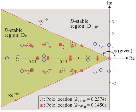
Figure 3. The $\mathcal{D}$-stable region $D_{\phi }$ and $D_{\mathrm{LHP}}$ for the locations of all nonzero poles of ${\mathcal{H}}_{\theta }\left(s\right)$.

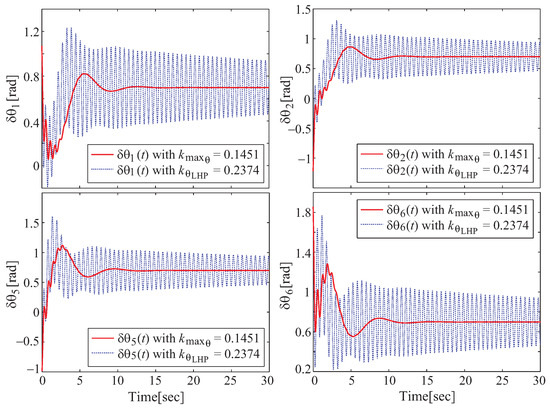
Figure 4. Time plots of $\delta {\theta }_i\left(t\right)$ ($i=1,2,5,6$) for $k_{\theta }=0.1451$ and $0.2374$.

Now the objective of this paper is to develop a novel Lyapunov $\mathcal{D}$-stabilization scheme that guarantees both (A1)–(A3) and the predesignated transient performance specifications for multi-agent dynamical systems in Figure 1 and Figure 2. To this end, a Lyapunov $\mathcal{D}$-stability problem is first defined, and the corresponding stability conditions are derived in Section 3. Next, an explicit Lyapunov $\mathcal{D}$-stabilization strategy for multi-agent dynamical systems exhibiting cyclic pursuit behavior is developed in Section 4.

3. Lyapunov $\mathcal{D}$-Stability Analysis of a Distributed Pursuit Formation Control System

In this section, a simple diagrammatic formation stability analysis scheme for distributed cooperative control for target-enclosing operations by multiple homogeneous dynamic agents is developed.

3.1. Lyapunov $\mathcal{D}$-Stability Problem

For the Lyapunov $\mathcal{D}$-stability analysis of the cyclic pursuit formation in multi-agent dynamical systems described in Section 2, (5) is first rewritten in the following vector form:

$${\dot{\mathbf{r}}}^{\theta }\left(t\right)=\left[\begin{array}{cccccc}-k_{\theta }& k_{\theta }& 0& 0& \cdots & 0\\ 0& -k_{\theta }& k_{\theta }& 0& \cdots & 0\\ 0& 0& \ddots & \ddots & 0& 0\\ ⋮& ⋮& \ddots & \ddots & \ddots & ⋮\\ 0& 0& \cdots & 0& -k_{\theta }& k_{\theta }\\ k_{\theta }& 0& \cdots & \cdots & 0& -k_{\theta }\end{array}\right]\mathit{\theta }\left(t\right)+\left[\begin{array}{c}0\\ 0\\ 0\\ ⋮\\ 0\\ 2k_{\theta }\pi \end{array}\right]·1=A_{\theta }\mathit{\theta }\left(t\right)+B_{\theta }·1,$$

(8)

where

$$\begin{array}{c}{A}_{\theta }:=\mathrm{circ}(-k_{\theta },k_{\theta },0,0,\cdots ,0)\in {\mathbb{R}}^{n\times n},\hfill \\ B_{\theta }:={[0,0,\cdots ,0,2k_{\theta }\pi ]}^T\in {\mathbb{R}}^n,\hfill \end{array}$$

$\mathit{\theta }:={[{\theta }_1,{\theta }_2,\cdots ,{\theta }_n]}^T\in {\mathbb{R}}^n$, ${\mathbf{r}}^{\theta }:={[r_1^{\theta },r_2^{\theta },\cdots ,r_n^{\theta }]}^T\in {\mathbb{R}}^n$, and “$\mathrm{circ}$” denotes the circulant matrix. Thus, the overall $\mathit{\theta }$-directional control scheme can be depicted as shown in Figure 5, where

$$h_{\theta }\left(s\right):=g_{\theta }\left(s\right)·{\displaystyle \frac{1}{s}}$$

(9)

is strictly proper owing to the properness of $g_{\theta }\left(s\right)$. Here, the eigenvalues ${\left\{{\lambda }_i\right\}}_{i=1}^n$ of $A_{\theta }$ can be written in the following form:

$${\lambda }_i=k_{\theta }\left[cos\left({\displaystyle \frac{2\pi (i-1)}{n}}\right)-1\right]+j{k}_{\theta }sin\left({\displaystyle \frac{2\pi (i-1)}{n}}\right),$$

(10)

where $j:=\sqrt{-1}$. Note that because $k_{\theta }>0$, $A_{\theta }$ has exactly one zero eigenvalue, ${\lambda }_1$, while the remaining $n-1$ eigenvalues ${\lambda }_i$ ($i=2,3,\cdots ,n$) lie strictly in the left-half complex plane. In the same manner, (6) and (7) can respectively be rewritten as follows:

$$\begin{array}{c}{\dot{\mathbf{r}}}^d\left(t\right)=A_d\mathit{d}\left(t\right)+B_d,\hfill \end{array}$$

(11)

$$\begin{array}{c}{\dot{\mathbf{r}}}^{\alpha }\left(t\right)=A_{\alpha }\mathit{\alpha }\left(t\right)+B_{\alpha },\hfill \end{array}$$

(12)

with $\mathit{d}:={[d_1,d_2,\cdots ,d_n]}^T\in {\mathbb{R}}^n$, $\mathit{\alpha }:={[{\alpha }_1,{\alpha }_2,\cdots ,{\alpha }_n]}^T$$\in {\mathbb{R}}^n$, $A_d:=-\mathrm{diag}(k_d,k_d,\cdots ,k_d)\in {\mathbb{R}}^{n\times n}$, $B_d:=\left(k_{d}D\right){\mathbf{1}}_n\in {\mathbb{R}}^n$, $A_{\alpha }:=-\mathrm{diag}(k_{\alpha },k_{\alpha },\cdots ,k_{\alpha })\in {\mathbb{R}}^{n\times n}$, $B_{\alpha }:=\left(k_{\alpha }\mathsf{\Phi }\right){\mathbf{1}}_n\in {\mathbb{R}}^n$, where ${\mathbf{1}}_n:={[1,1,\cdots ,1]}^T\in {\mathbb{R}}^n$. The block diagrams of $\mathit{d}$- and $\mathit{\alpha }$-directional formation control systems have the same form as that in Figure 5.

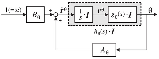
Figure 5. Block diagram of the $\mathit{\theta }$-directional formation-controlled system: ${\mathcal{H}}_{\theta }\left(s\right)$.

In Figure 5, the transfer function ${\mathcal{H}}_{\theta }\left(s\right)$ from the input “c” to $\mathit{\theta }$ is obtained as

$${\displaystyle {\mathcal{H}}_{\theta }\left(s\right)={\left(\frac{1}{h_{\theta }\left(s\right)}{I}_n-A_{\theta }\right)}^{-1}{B}_{\theta }.}$$

(13)

It then follows from (13) that

$${\mathcal{H}}_{\theta }\left(s\right)=L_{\theta }\left({\varphi }_{\theta }\left(s\right)\right),{\varphi }_{\theta }\left(s\right):=1/h_{\theta }\left(s\right),$$

(14)

where $L_{\theta }\left(s\right)={(s{I}_n-A_{\theta })}^{-1}{B}_{\theta }$. Note that ${\varphi }_{\theta }\left(0\right)=0$ from (9). Hence, the transformed transfer function ${\mathcal{H}}_{\theta }\left(s\right)=L_{\theta }\left({\varphi }_{\theta }\left(s\right)\right)$ of $L_{\theta }\left(s\right)$ is said to have a generalized frequency variable ${\varphi }_{\theta }\left(s\right)$ (see [23,24] for details). Similarly, the $\mathit{d}$- and $\mathit{\alpha }$-directional transfer functions ${\mathcal{H}}_d\left(s\right)$ and ${\mathcal{H}}_{\alpha }\left(s\right)$ can be derived as follows:

$$\begin{array}{cc}\hfill & {\mathcal{H}}_d\left(s\right)=L_d\left({\varphi }_d\left(s\right)\right),{\varphi }_d\left(s\right):=1/h_d\left(s\right)=s/g_d\left(s\right),\hfill \end{array}$$

(15)

$$\begin{array}{cc}\hfill & {\mathcal{H}}_{\alpha }\left(s\right)=L_{\alpha }\left({\varphi }_{\alpha }\left(s\right)\right),{\varphi }_{\alpha }\left(s\right):=1/h_{\alpha }\left(s\right)=s/g_{\alpha }\left(s\right).\hfill \end{array}$$

(16)

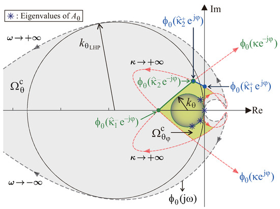
For the sake of clarity, hereinafter, the focus will primarily be on the $\theta$-directional stabilization scheme. Based on the above system description, the following Lyapunov $\mathcal{D}$-stability problem is considered. All the poles of ${\mathcal{H}}_{\theta }\left(s\right)$, except for one pole at the origin, are assigned to a predesignated region of the complex plane, or a $\mathcal{D}$-stability region, which is formulated as follows:

Problem A:

(Lyapunov $\mathcal{D}$-stability problem) Derive a Lyapunov $\mathcal{D}$-stability criterion for θ-directional global pursuit formation that determines whether all the nonzero poles of ${\mathcal{H}}_{\theta }\left(s\right)$, as expressed in (13), belong to a predesignated $\mathcal{D}$-stable region, $D_{\phi }$, as shown in Figure 3. This region is characterized as follows:

$$D_{\phi }:=\{s:=\kappa e^{j\widehat{\phi }}\in \mathbb{C}:\phi <\widehat{\phi }<2\pi -\phi ,\forall \kappa >0\},$$

(17)

where $\mathbb{C}$ denotes the set of complex numbers, and φ, satisfying $\pi /2\le \phi <\pi$, is assumed to be given a priori.

In the following subsection, a Lyapunov $\mathcal{D}$-stability condition is derived to guarantee the pole assignment of ${\mathcal{H}}_{\theta }\left(s\right)$ as specified in “Problem A”.

3.2. Lyapunov $\mathcal{D}$-Stability Criterion

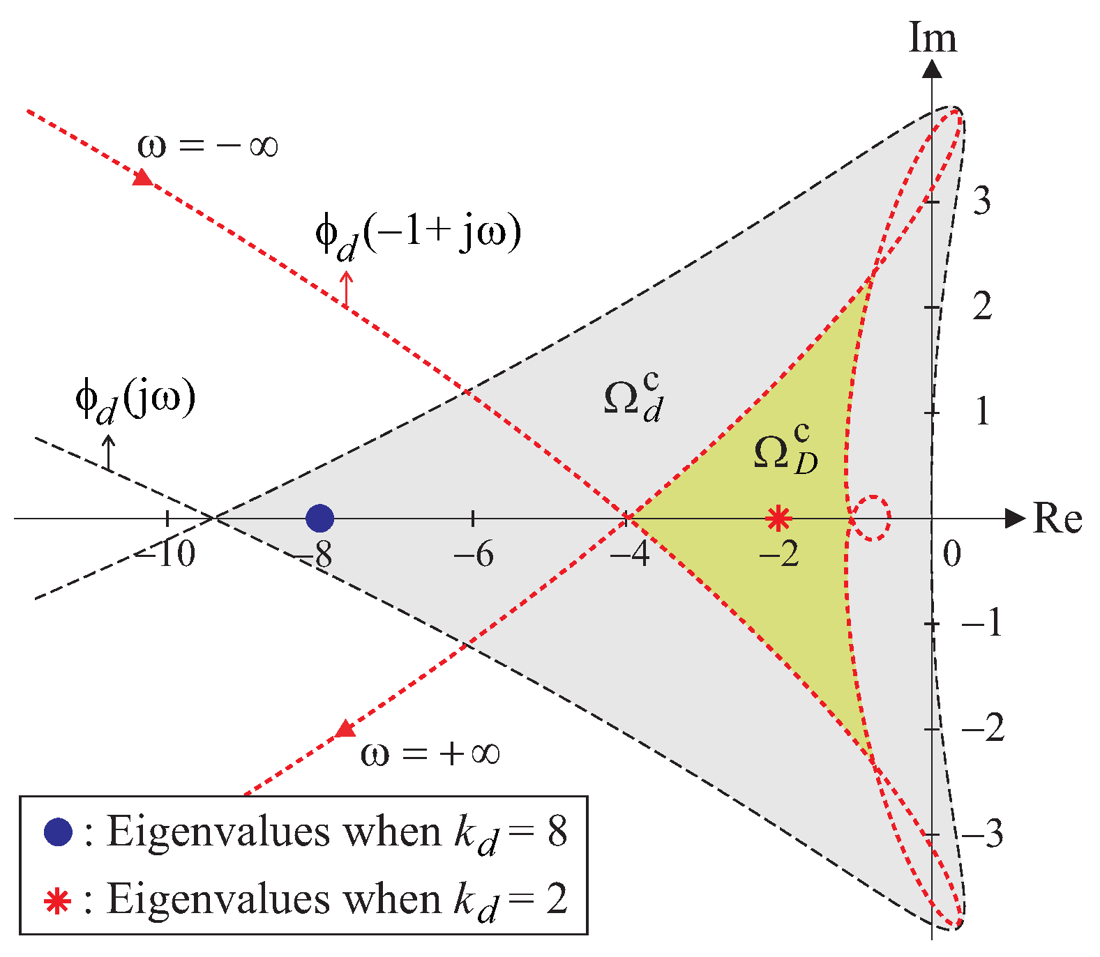
Let two domains ${\Omega }_{{\theta }_{\phi }}$ and ${\Omega }_{{\theta }_{\phi }}^{\mathrm{c}}$ in the complex plane be defined as follows (These are the generalizations of domains such that ${\Omega }_{\theta }:={\varphi }_{\theta }\left({\mathbb{C}}_{+}\right)$ and ${\Omega }_{\theta }^{\mathrm{c}}:=\mathbb{C}\backslash {\Omega }_{\theta }$, where ${\mathbb{C}}_{+}=\{s\in \mathbb{C}:Re\left[s\right]\ge 0\}$, which are defined in [22]):

$${\Omega }_{{\theta }_{\phi }}:={\varphi }_{\theta }\left({\mathbb{C}}_{\phi }\right),{\Omega }_{{\theta }_{\phi }}^{\mathrm{c}}:=\mathbb{C}\backslash {\Omega }_{\phi },$$

(18)

where

$${\mathbb{C}}_{\phi }=\{s:=\kappa e^{j\vartheta }\in \mathbb{C}:-\phi \le \vartheta \le \phi ,\forall \kappa \ge 0\}.$$

Note that the domain ${\Omega }_{{\theta }_{\phi }}^{\mathrm{c}}$ does not include the origin of the complex plane. Further, $A_{\theta }$ has one eigenvalue at the origin, which implies that the set of poles of ${\mathcal{H}}_{\theta }\left(s\right)$ includes all the poles of $h_{\theta }\left(s\right)$. These facts immediately give the following condition as a necessary condition for the solvability of Problem A.

Assumption 1.

The closed-loop transfer function $g_{\theta }\left(s\right)$ defined by (2) is proper and stable and has no zero at the origin of the complex plane.

The key result for this investigation, which provides the Lyapunov $\mathcal{D}$-stability criterion for ${\mathcal{H}}_{\theta }\left(s\right)$ as defined in “Problem A”, is then obtained as follows:

Proposition 1.

Suppose that $g_{\theta }\left(s\right)$ defined by (2) satisfies Assumption 1. Then, the following statements are equivalent:

(i) 

One of the eigenvalues of $A_{\theta }$ is at the origin of the complex plane, and the remaining eigenvalues belong to the domain ${\Omega }_{{\theta }_{\phi }}^{\mathrm{c}}$ defined by (18) (see Figure 6).

Figure 6. Imageof ${\varphi }_{\theta }\left(\kappa e^{\pm j\phi }\right)$ and the corresponding domain ${\Omega }_{{\theta }_{\phi }}^{\mathrm{c}}$.

(ii) 

One of the poles of ${\mathcal{H}}_{\theta }\left(s\right)$ is at the origin of the complex plane, and the remaining poles belong to the $\mathcal{D}$-stable region ${\mathrm{D}}_{\phi }$ defined by (17) (see Figure 3).

It is proved in the same manner as Proposition 4.1 in [22] and is therefore omitted here. This proposition means that the Lyapunov $\mathcal{D}$-stability of ${\mathcal{H}}_{\theta }\left(s\right)$ in “Problem A” can be judged diagrammatically by just looking at the locations of the eigenvalues of $A_{\theta }$ depending on $k_{\theta }$ in relation to a domain ${\Omega }_{{\theta }_{\phi }}^{\mathrm{c}}$, which is determined by using $h_{\theta }\left(s\right)$ in (9). In particular, Proposition 1 indicates that ${\mathcal{H}}_{\theta }\left(s\right)$ has one pole at the origin and all other poles in the predesignated region ${\mathrm{D}}_{\phi }$ (i.e., ${\mathcal{H}}_{\theta }\left(s\right)$ is Lyapunov $\mathcal{D}$-stable), if all the eigenvalues of $A_{\theta }$ except one zero eigenvalue belong to the domain ${\Omega }_{{\theta }_{\phi }}^{\mathrm{c}}$.

The situation for the d- and $\alpha$-directional stability is slightly different. Because $A_d$ in (11) and $A_{\alpha }$ in (12) have n multiple eigenvalues at ($-k_d+j0$) and ($-k_{\alpha }+j0$), respectively, the asymptotic stability can be analyzed by using the scheme given in [23], i.e., the necessary and sufficient asymptotic stability condition for ${\mathcal{H}}_d\left(s\right)$ (${\mathcal{H}}_{\alpha }\left(s\right)$) is that all eigenvalues of $A_d$ ($A_{\alpha }$) belong to the domain ${\Omega }_d^{\mathrm{c}}$ (${\Omega }_{\alpha }^{\mathrm{c}}$) defined as ${\Omega }_d:={\varphi }_d\left({\mathbb{C}}_{+}\right)$, ${\Omega }_d^{\mathrm{c}}:=\mathbb{C}\backslash {\Omega }_d$ and ${\Omega }_{\alpha }:={\varphi }_{\alpha }\left({\mathbb{C}}_{+}\right)$, ${\Omega }_{\alpha }^{\mathrm{c}}:=\mathbb{C}\backslash {\Omega }_{\alpha }$ (see [22]).

From Proposition 1 and Theorems 5.1 and 5.2 in [22], the following key properties are guaranteed:

(I) If ${\mathcal{H}}_{\theta }\left(s\right)$ is Lyapunov $\mathcal{D}$-stable (i.e., the condition in Proposition 1 is satisfied), then the control objective ($A1$) for target-enclosing formation is achieved.

(II) If ${\mathcal{H}}_d\left(s\right)$ and ${\mathcal{H}}_{\alpha }\left(s\right)$ are asymptotically stable, then the control objectives (A2) and (A3) are achieved.

The analysis presented in this section demonstrates a practical and theoretically grounded approach to ensuring that ${\mathcal{H}}_{\theta }\left(s\right)$ in (13) is Lyapunov $\mathcal{D}$-stable. Specifically, rather than directly computing all the poles of ${\mathcal{H}}_{\theta }\left(s\right)$ to verify their inclusion within the $\mathcal{D}$-stable region ${\mathrm{D}}_{\phi }$, this section establishes a more efficient and scalable method leveraging key properties of individual agent dynamics and the system configuration. The process involves the following steps:

• STEP 1. Define the agent dynamics: Start by defining $h_{\theta }\left(s\right)$ using the individual agent dynamics $g_{\theta }\left(s\right)$ of (2) as specified in (9).
• STEP 2. Determine ${\varphi }_{\theta }\left(s\right)$: Using $h_{\theta }\left(s\right)$, compute ${\varphi }_{\theta }\left(s\right)$ as defined in (14).
• STEP 3. Derive ${\Omega }_{{\theta }_{\phi }}^{\mathrm{c}}$: Use ${\varphi }_{\theta }\left(s\right)$ to derive the domain ${\Omega }_{{\theta }_{\phi }}^{\mathrm{c}}$, which is specified in (18).
• STEP 4. Specify $k_{\theta }$ and compute eigenvalues: Select a specific value for the connectivity gain $k_{\theta }$, and calculate the eigenvalues of the matrix $A_{\theta }$, which incorporates $k_{\theta }$.
• STEP 5. Verify inclusion: Check whether all eigenvalues of $A_{\theta }$, excluding the one located at the origin, lie within the domain ${\Omega }_{{\theta }_{\phi }}^{\mathrm{c}}$. If they do, the system ${\mathcal{H}}_{\theta }\left(s\right)$ is Lyapunov $\mathcal{D}$-stable. Otherwise, it is not.

This systematic process, centered around the eigenvalue analysis of $A_{\theta }$, is the core contribution of this section and enables a practical evaluation of $\mathcal{D}$-stability for a given $k_{\theta }$. However, while this diagrammatic method provides a practical mechanism for verifying $\mathcal{D}$-stability for a specific $k_{\theta }$, it faces limitations when determining the maximum connectivity gain, $k_{{max}_{\theta }}$, that guarantees $\mathcal{D}$-stability. Relying on trial-and-error approaches by manually varying $k_{\theta }$ would be computationally intensive and unlikely to yield the precise value of $k_{{max}_{\theta }}$.

To address this critical limitation, Section 4 introduces a systematic and computationally efficient optimization framework to derive the upper bound $k_{{max}_{\theta }}$ for $k_{\theta }$. This framework leverages the GKYP lemma and reformulates the problem into a numerically tractable LMI optimization problem. By systematically solving for $k_{{max}_{\theta }}$, this approach overcomes the challenges associated with diagrammatic methods and enables the accurate and efficient determination of connectivity gains that ensure Lyapunov $\mathcal{D}$-stability.

4. Lyapunov $\mathcal{D}$-Stabilization: GKYP Lemma-Based Scheme

4.1. Lyapunov $\mathcal{D}$-Stabilization Problem

In Proposition 1, a considerably simple diagrammatic Lyapunov $\mathcal{D}$-stability criterion was derived. The focus here is to determine the maximum permissible limit of the connectivity gain $k_{\theta }$ that satisfies the requirement presented in “Problem A” in the previous section. Accordingly, the following Lyapunov $\mathcal{D}$-stabilization problem is considered in this section:

Problem S: Determine the upper bound $k_{{max}_{\theta }}(>0)$ guaranteeing the following requirement: for any number of agents $n(>0)$ and the connectivity gain $k_{\theta }\in (0,k_{{max}_{\theta }})$ in (8), all nonzero poles of ${\mathcal{H}}_{\theta }\left(s\right)$ in (13) are placed within the predesignated $\mathcal{D}$-stable region ${\mathrm{D}}_{\phi }$, as defined in (17) and illustrated in Figure 3.

The condition that guarantees that all nonzero eigenvalues of $A_{\theta }$ with sufficiently large n belong to the domain ${\Omega }_{{\theta }_{\phi }}^{\mathrm{c}}$ characterized by $\kappa e^{\pm j\phi }$ is derived from Proposition 1 and Figure 6 as follows:

$${({\varphi }_{{\theta }_{\phi }}^{\mathrm{Re}}\left(\kappa \right)+k_{\theta })}^2+{\left({\varphi }_{{\theta }_{\phi }}^{\mathrm{Im}}\left(\kappa \right)\right)}^2>k_{\theta }^2,\forall \kappa >0,$$

(19)

where ${\varphi }_{{\theta }_{\phi }}^{\mathrm{Re}}\left(\kappa \right)$ and ${\varphi }_{{\theta }_{\phi }}^{\mathrm{Im}}\left(\kappa \right)$ are respectively defined as

$${\varphi }_{{\theta }_{\phi }}^{\mathrm{Re}}\left(\kappa \right):=\mathrm{Re}\left[{\varphi }_{\theta }\left(\kappa e^{j\phi }\right)\right],{\varphi }_{{\theta }_{\phi }}^{\mathrm{Im}}\left(\kappa \right):=\mathrm{Im}\left[{\varphi }_{\theta }\left(\kappa e^{j\phi }\right)\right],$$

and $\phi$ is assumed to be given in advance by the designer. It can readily be found from (19) that

$${({\varphi }_{\theta }\left(\kappa e^{j\phi }\right)+k_{\theta })}^{*}({\varphi }_{\theta }\left(\kappa e^{j\phi }\right)+k_{\theta })>k_{\theta }^2$$

(20)

is equivalent to the the following inequality condition: for $\forall \kappa >0$,

$${\left[\begin{array}{c}{h}_{\theta }\left(\kappa e^{j\phi }\right)\\ 1\end{array}\right]}^{*}\mathsf{\Pi }\left[\begin{array}{c}{h}_{\theta }\left(\kappa e^{j\phi }\right)\\ 1\end{array}\right]<0,\mathsf{\Pi }:=\left[\begin{array}{cc}0& -k_{\theta }\\ -k_{\theta }& -1\end{array}\right].$$

(21)

Therefore, the optimization problem to find the upper bound $k_{{max}_{\theta }}$ of connectivity gain $k_{\theta }$ satisfying the requirement in “Problem S” can be formulated as follows:

$$\begin{array}{c}{k}_{{max}_{\theta }}:=arg\underset{k_{\theta },\kappa }{sup}{k}_{\theta }\mathrm{subject} \mathrm{to} \left(21\right) \mathrm{and}{k}_{\theta }>0.\hfill \end{array}$$

(22)

Once the upper bound $k_{{max}_{\theta }}$ is obtained, all nonzero poles of ${\mathcal{H}}_{\theta }\left(s\right)$ in (13) can be assigned in the predesignated $\mathcal{D}$-stable region ${\mathrm{D}}_{\phi }$ by setting $k_{\theta }$ in $A_{\theta }$ of (8) as guaranteeing $0<k_{\theta }<k_{{max}_{\theta }}$. However, the above optimization problem may not be easily solved because the constraint condition (21) should be checked for all $\kappa$(>0) and the inequality always fails for $\kappa =0$.

4.2. LMI Solution for Lyapunov $\mathcal{D}$-Stabilization

To overcome the aforementioned difficulty, the inequality condition (21) is converted into LMIs using the GKYP lemma [26,27]. It is important to note that the corresponding LMI optimization problem is numerically tractable and can be solved efficiently. Assume now that the state–space realization of $h_{\theta }\left(s\right)$ is expressed as

$$h_{\theta }\left(s\right)=C_{h_{\theta }}{(sI-A_{h_{\theta }})}^{-1}{B}_{h_{\theta }}+D_{h_{\theta }}.$$

(23)

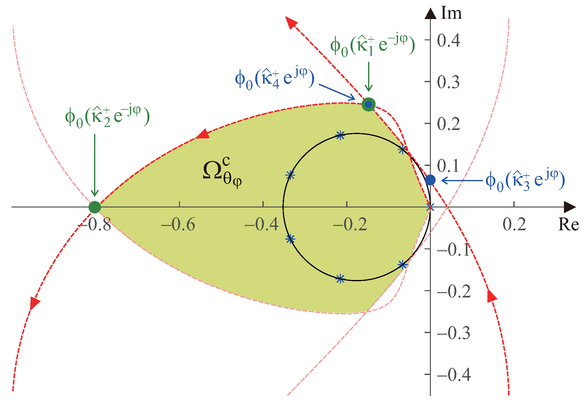
In formulating such an optimization problem, the characterization of the restricted ranges of $\kappa$, which are key factors in checking the constraint condition (21) within the framework of the GKYP lemma, must be approached with utmost caution. For given $\phi (>0)$ and ${\varphi }_{\theta }\left(s\right)(=1/h_{\theta }\left(s\right))$, both ${\varphi }_{\theta }\left(\kappa e^{j\phi }\right)$ and ${\varphi }_{\theta }\left(\kappa e^{-j\phi }\right)$ are readily obtained (see Figure 6). Then, using ${\varphi }_{\theta }\left(\kappa e^{\pm j\phi }\right)$, the domain ${\Omega }_{{\theta }_{\phi }}^{\mathrm{c}}$ is determined as described in (18). Consequently, in the optimization problem aimed at determining the maximum value of the radius $k_{\theta }$ of the circle on which the eigenvalues ${\left\{{\lambda }_i\right\}}_{i=1}^n$ of $A_{\theta }$ are located, multiple intervals of $\kappa$ must be carefully selected based on the shape of ${\Omega }_{{\theta }_{\phi }}^{\mathrm{c}}$. It is crucial that the circle with radius $k_{\theta }(>0)$, where the eigenvalues lie on its circumference, remains entirely within the interior of ${\Omega }_{{\theta }_{\phi }}^{\mathrm{c}}$. Note that because $A_{\theta }$ has exactly one zero eigenvalue, the center of the circle is at $(-k_{\theta },0)$, and such a circle is symmetric about the real axis. The domain ${\Omega }_{{\theta }_{\phi }}^{\mathrm{c}}$ is also symmetric about the real axis. Therefore, the restricted multiple ranges of $\kappa$ used in the optimization procedure can be determined by considering only the portion corresponding to the second quadrant of the complex plane, without needing to characterize the entire domain ${\Omega }_{{\theta }_{\phi }}^{\mathrm{c}}$.

Now, suppose a certain dynamical multi-agent system produces the ${\varphi }_{\theta }\left(\kappa e^{\pm j\phi }\right)$ and the domain ${\Omega }_{{\theta }_{\phi }}^{\mathrm{c}}$ shown in Figure 6. The determination of valid multiple intervals of $\kappa$ can then be examined. The portion of ${\Omega }_{{\theta }_{\phi }}^{\mathrm{c}}$ corresponding to the second quadrant of the complex plane indicates that it is sufficient to check the condition (21) in two intervals of $\kappa$, such as ${\widehat{\kappa }}_1^{+}\le \kappa \le {\widehat{\kappa }}_2^{+}$ and ${\widehat{\kappa }}_1^{-}\le \kappa \le {\widehat{\kappa }}_2^{-}$, where ${\widehat{\kappa }}_{*}^{+}$ corresponds to a certain point on the line segment represented by ${\varphi }_{\theta }\left(\kappa e^{j\phi }\right)$ with $\forall \kappa >0$, and ${\widehat{\kappa }}_{*}^{-}$ corresponds similarly to a point on the line segment represented by ${\varphi }_{\theta }\left(\kappa e^{-j\phi }\right)$. Generalizing this, the set of complex numbers, $\mathsf{\Lambda }(\mathsf{\Gamma },\mathsf{\Psi })$, which is composed of ${\mathsf{\Lambda }}_i^{+}({\mathsf{\Gamma }}_{+},{\mathsf{\Psi }}_i^{+})$ corresponding to ${\widehat{\kappa }}_{2i-1}^{+}\le \kappa \le {\widehat{\kappa }}_{2i}^{+}$ for $i=1,2,\cdots ,N_p$ and ${\mathsf{\Lambda }}_i^{-}({\mathsf{\Gamma }}_{-},{\mathsf{\Psi }}_j^{-})$ corresponding to ${\widehat{\kappa }}_{2j-1}^{+}\le \kappa \le {\widehat{\kappa }}_{2j}^{+}$ for $j=1,2,\cdots ,N_n$, can be defined as follows:

$$\mathsf{\Lambda }(\mathsf{\Gamma },\mathsf{\Psi }):=\left(\stackrel{N_p}{\bigcup _{i=1}}{\mathsf{\Lambda }}_i^{+}({\mathsf{\Gamma }}_{+},{\mathsf{\Psi }}_i^{+})\right)\cup \left(\stackrel{N_n}{\bigcup _{j=1}}{\mathsf{\Lambda }}_j^{-}({\mathsf{\Gamma }}_{-},{\mathsf{\Psi }}_j^{-})\right),$$

(24)

where

$$\begin{array}{ccc}& & {\mathsf{\Lambda }}_i^{+}({\mathsf{\Gamma }}_{+},{\mathsf{\Psi }}_i^{+}):=\left\{\lambda \in \mathbb{C}:{\left[\begin{array}{c}\lambda \\ 1\end{array}\right]}^{*}{\mathsf{\Gamma }}_{+}\left[\begin{array}{c}\lambda \\ 1\end{array}\right]=0,{\left[\begin{array}{c}\lambda \\ 1\end{array}\right]}^{*}{\mathsf{\Psi }}_i^{+}\left[\begin{array}{c}\lambda \\ 1\end{array}\right]\ge 0\right\},\hfill \end{array}$$

(25)

$$\begin{array}{ccc}& & {\mathsf{\Lambda }}_j^{-}({\mathsf{\Gamma }}_{-},{\mathsf{\Psi }}_j^{-}):=\left\{\lambda \in \mathbb{C}:{\left[\begin{array}{c}\lambda \\ 1\end{array}\right]}^{*}{\mathsf{\Gamma }}_{-}\left[\begin{array}{c}\lambda \\ 1\end{array}\right]=0,{\left[\begin{array}{c}\lambda \\ 1\end{array}\right]}^{*}{\mathsf{\Psi }}_j^{-}\left[\begin{array}{c}\lambda \\ 1\end{array}\right]\ge 0\right\}\hfill \end{array}$$

(26)

with

$$\begin{array}{cc}& {\mathsf{\Gamma }}_{+}:=\left[\begin{array}{cc}0& tan\phi -j\\ tan\phi +j& 0\end{array}\right],{\mathsf{\Gamma }}_{-}:=\left[\begin{array}{cc}0& tan(-\phi )-j\\ tan(-\phi )+j& 0\end{array}\right],\end{array}$$

(27)

$$\begin{array}{cc}& {\mathsf{\Psi }}_i^{+}:=\left[\begin{array}{cc}-1& {\lambda }_{c_i}^{+}\\ {\overline{\lambda }}_{c_i}^{+}& -{\widehat{\kappa }}_{2i-1}^{+}·{\widehat{\kappa }}_{2i}^{+}\end{array}\right],{\mathsf{\Psi }}_j^{-}:=\left[\begin{array}{cc}-1& {\lambda }_{c_j}^{-}\\ {\overline{\lambda }}_{c_j}^{-}& -{\widehat{\kappa }}_{2j-1}^{-}·{\widehat{\kappa }}_{2j}^{-}\end{array}\right]\end{array}$$

(28)

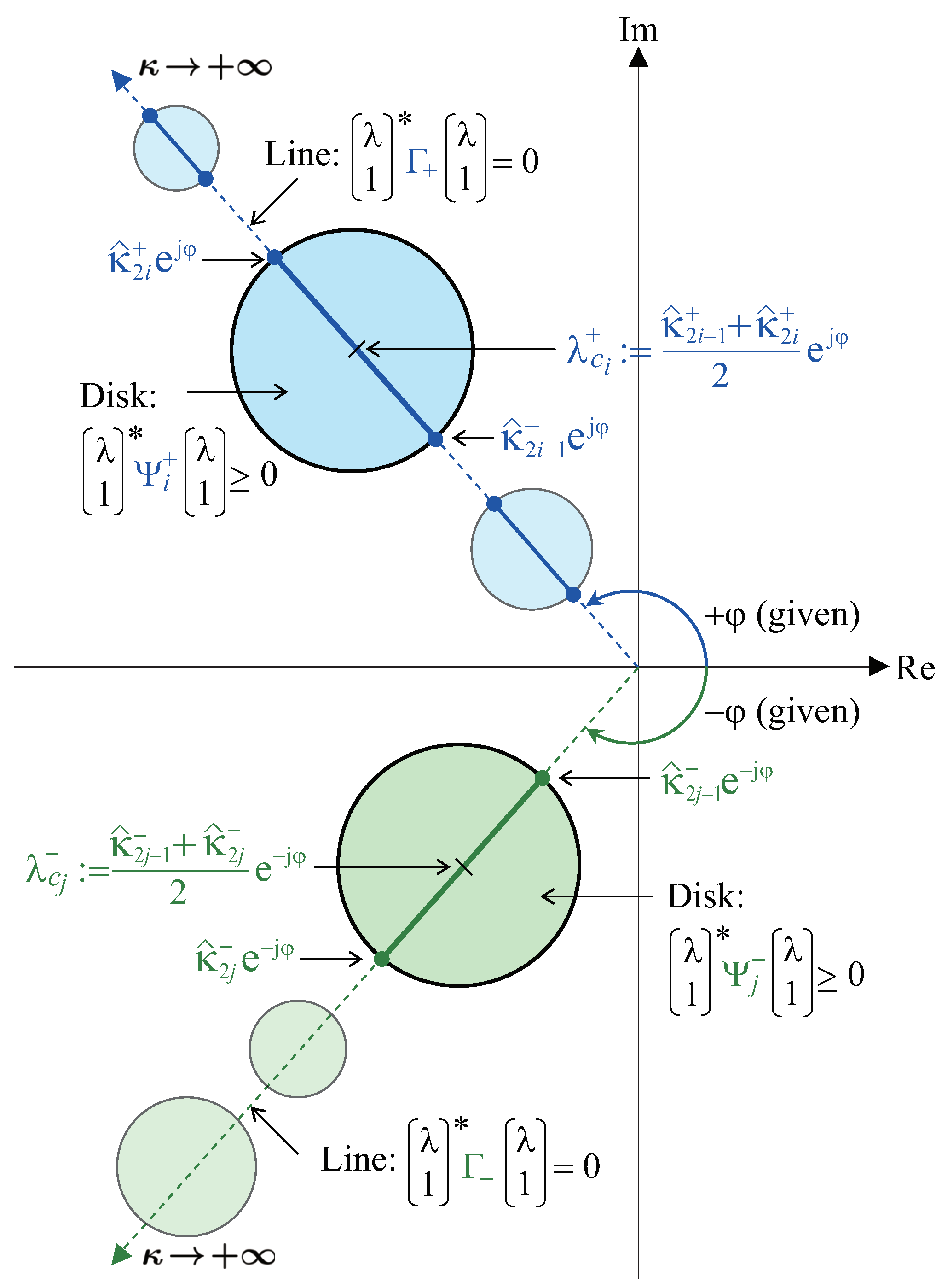
for ${\lambda }_{c_i}^{+}:={\displaystyle \frac{{\widehat{\kappa }}_{2i-1}^{+}+{\widehat{\kappa }}_{2i}^{+}}{2}}{e}^{j\phi }$ and ${\lambda }_{c_j}^{-}:={\displaystyle \frac{{\widehat{\kappa }}_{2j-1}^{-}+{\widehat{\kappa }}_{2j}^{-}}{2}}{e}^{-j\phi }$ (see Figure 7). For details regarding the choices of ${\mathsf{\Gamma }}^{\pm }$ and ${\mathsf{\Psi }}_{*}^{\pm }$, readers are requested to refer to [27]. Therefore, under the setting (24) with (25)–(28) the upper bound $k_{{max}_{\theta }}$ of $k_{\theta }$ mentioned in “Problem S” can easily be obtained by solving the following optimization problem subject to LMI constraint conditions:

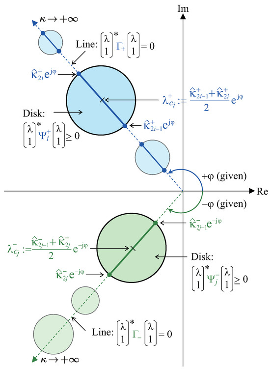
Figure 7. Set of complex numbers determined by $\mathsf{\Lambda }(\mathsf{\Gamma },\mathsf{\Psi })$ in (24).

Optimization problem for Problem S:

Given $h_{\theta }\left(s\right)\sim (A_{h_{\theta }},B_{h_{\theta }},C_{h_{\theta }},D_{h_{\theta }})$ and φ ($\pi /2\le \phi <\pi$), solve

$$k_{{max}_{\theta }}:=arg\underset{k_{\theta },P^{\pm }\in {\mathbf{H}}_n,Q^{\pm }\in {\mathbf{H}}_n}{sup}{k}_{\theta },$$

(29)

where ${\mathbf{H}}_n$ denotes an $n\times n$ Hermitian matrix, subject to $k_{\theta }>0$ and

$$\begin{array}{ccc}& & Q^{+}>0,M_1^{*}{Z}_i^{+}{M}_1+M_2^{*}\mathsf{\Pi }{M}_2<0(i=1,2,\cdots ,N_p),\hfill \end{array}$$

(30)

$$\begin{array}{ccc}& & Q^{-}>0,M_1^{*}{Z}_j^{-}{M}_1+M_2^{*}\mathsf{\Pi }{M}_2<0(j=1,2,\cdots ,N_n),\hfill \end{array}$$

(31)

where $Z_i^{+}:={\mathsf{\Gamma }}_{+}\otimes P^{+}+{\mathsf{\Psi }}_i^{+}\otimes Q^{+}$ and $Z_j^{-}:={\mathsf{\Gamma }}_{-}\otimes P^{-}+{\mathsf{\Psi }}_j^{-}\otimes Q^{-}$ with Π defined by (21), and ${\mathsf{\Gamma }}_{\pm }$ and ${\mathsf{\Psi }}_{*}^{\pm }$ defined by (27) and (28), and

$$M_1:=\left[\begin{array}{cc}{A}_{h_{\theta }}& B_{h_{\theta }}\\ I& 0\end{array}\right],M_2:=\left[\begin{array}{cc}{C}_{h_{\theta }}& D_{h_{\theta }}\\ 0& I\end{array}\right].$$

(32)

Note that the LMI constraint conditions in (30) and (31), which are equivalent to (21), are derived using the GKYP lemma [26,27]. If one obtains $k_{{max}_{\theta }}$ from the above optimization scheme and then sets $k_{\theta }$ in (8) as guaranteeing $0<k_{\theta }<k_{{max}_{\theta }}$, all nonzero poles of ${\mathcal{H}}_{\theta }\left(s\right)$ in (13) are placed in the predesignated $\mathcal{D}$-stable region, ${\mathrm{D}}_{\phi }$, in Figure 3.

The optimization problem introduced above provides a systematic approach to determining the maximum connectivity gain, $k_{\theta }$, that ensures $\mathcal{D}$-stability for the multi-agent system. While the formulation presents the critical LMI constraints and optimization structure, it is essential to outline the precise steps involved in deriving $k_{{max}_{\theta }}$ from the system dynamics and stability requirements. To enhance clarity and reproducibility, the following step-by-step procedure outlines how the proposed methodology systematically transforms the $\mathcal{D}$-stability criterion into a computationally efficient optimization framework and ultimately determines $k_{{max}_{\theta }}$.

Steps for Deriving the Connectivity Gain Upper Bound $k_{{max}_{\theta }}$:

• STEP 1. Define the agent dynamics and stability requirements: Start with the agent dynamics $g_{\theta }\left(s\right)$ represented as (2). Define $h_{\theta }\left(s\right)$ in (9) derived from $g_{\theta }\left(s\right)$. The $\mathcal{D}$-stability criterion requires all poles of ${\mathcal{H}}_{\theta }\left(s\right)$ to lie within the $\mathcal{D}$-stable region ${\mathrm{D}}_{\phi }$ for a given $\phi$ (see Figure 3). Once $h_{\theta }\left(s\right)$ is defined, obtain its state–space realization as shown in (23).
• STEP 2. Formulate the function ${\varphi }_{\theta }\left(s\right)$: Compute ${\varphi }_{\theta }\left(s\right)$ as the inverse of $h_{\theta }\left(s\right)$, as specified in (14). This transformation is essential for defining the domain ${\Omega }_{{\theta }_{\phi }}^{\mathrm{c}}$.
• STEP 3. Define the domain ${\Omega }_{{\theta }_{\phi }}^{\mathrm{c}}$ for eigenvalues: Using ${\varphi }_{\theta }\left(s\right)$, derive the domain ${\Omega }_{{\theta }_{\phi }}^{\mathrm{c}}$ in the complex plane by following (18). This domain specifies where the eigenvalues of $A_{\theta }$ must reside to ensure ${\mathcal{H}}_{\theta }\left(s\right)$ satisfies the $\mathcal{D}$-stability criterion.
• STEP 4. Determine the relevant intervals of $\kappa$ for eigenvalue inclusion: The eigenvalues of $A_{\theta }$, which depend on $k_{\theta }$, lie on a circle in the complex plane centered at $(-k_{\theta },0)$ with a radius of $k_{\theta }$ as shown in (10). To ensure these eigenvalues (except the one at the origin) lie within ${\Omega }_{{\theta }_{\phi }}^{\mathrm{c}}$, identify the specific portions of ${\Omega }_{{\theta }_{\phi }}^{\mathrm{c}}$ that are critical for eigenvalue inclusion. Using the boundary of ${\Omega }_{{\theta }_{\phi }}^{\mathrm{c}}$ described by ${\varphi }_{\theta }\left(\kappa e^{\pm j\phi }\right)$, determine the intervals of $\kappa$ that define the relevant boundary conditions. For example, as shown in Figure 6, two intervals of $\kappa$ might be identified, such as: ${\widehat{\kappa }}_1^{+}\le \kappa \le {\widehat{\kappa }}_2^{+}$ and ${\widehat{\kappa }}_1^{-}\le \kappa \le {\widehat{\kappa }}_2^{-}$. The values of ${\widehat{\kappa }}_1^{+}$, ${\widehat{\kappa }}_2^{+}$, ${\widehat{\kappa }}_1^{-}$ and ${\widehat{\kappa }}_2^{-}$ are computed to specify the portions of the boundary that must be considered in subsequent steps.
• STEP 5. Set up the LMI-based optimization problem: Using the intervals of $\kappa$ determined in STEP 4, formulate the Linear Matrix Inequality (LMI) constraints and the optimization objective to determine the upper bound $k_{{max}_{\theta }}$. This includes:
  • Computing ${\mathsf{\Psi }}_{*}^{\pm }$ in (28) using the intervals of $\kappa$.
  • Defining ${\mathsf{\Gamma }}_{\pm }$ in (27) using the given $\phi$ to represent the $\mathcal{D}$-stable region.
  • Utilizing the state–space realization of $h_{\theta }\left(s\right)$ in (23) to compute $M_1$ and $M_2$ in (32).
  Combinethese elements to define the optimization problem for Problem S in (29)–(31). The objective function maximizes $k_{\theta }$, constrained by the LMI conditions derived from the GKYP lemma.
• STEP 6. Solve the optimization problem: Using numerical solvers such as MATLAB’s LMI toolbox (version 20230622), solve the optimization problem to compute the maximum value of $k_{\theta }$ (i.e., $k_{{max}_{\theta }}$) that satisfies the $\mathcal{D}$-stability constraints. This step provides a systematic way to determine the largest connectivity gain that ensures the desired stability.
• STEP 7. Verify the result with eigenvalue analysis (optional): As a verification step, evaluate the eigenvalues of $A_{\theta }$ for $k_{{max}_{\theta }}$ to confirm that they reside within the domain ${\Omega }_{{\theta }_{\phi }}^{\mathrm{c}}$ (excluding the eigenvalue at the origin). This optional check validates the correctness of the computed $k_{{max}_{\theta }}$.

Note that this systematic process overcomes the limitations of the diagrammatic method discussed in Section 3.2 by providing a computationally efficient framework to accurately determine $k_{{max}_{\theta }}$. The proposed optimization problem not only ensures the Lyapunov $\mathcal{D}$-stability of the multi-agent system but also streamlines the process, making it scalable and practical for real-world applications.

The proposed LMI optimization approach offers a significant computational advantage in large-scale multi-agent systems by maintaining constant complexity irrespective of the number of agents, n. This efficiency is achieved through a focus on individual agent dynamics rather than the collective system dynamics, thereby avoiding the computational overhead typically associated with large-scale systems.

To illustrate this, consider a multi-agent system where each agent is governed by $\nu$-th order dynamics, realized in state–space as $h_{\theta }\left(s\right)\sim (A_{h_{\theta }},B_{h_{\theta }},C_{h_{\theta }},D_{h_{\theta }})$. For a system with n agents, the combined system dynamics, ${\mathcal{H}}_{\theta }\left(s\right)$. For such a system with n agents, the overall system dynamics, ${\mathcal{H}}_{\theta }\left(s\right)$, when realized in state–space form, result in matrices of dimensions ${\mathcal{A}}_{h_{\theta }}\in {\mathbb{R}}^{\nu n\times \nu n}$ and ${\mathcal{B}}_{h_{\theta }}\in {\mathbb{R}}^{\nu n}$. Consequently, direct $\mathcal{D}$-stability analysis based on the entire system dynamics would require substantial computational resources, especially as n increases, since the eigenvalue computation of the high-dimensional matrix ${\mathcal{A}}_{h_{\theta }}\in {\mathbb{R}}^{\nu n\times \nu n}$ and related operations scale with the matrix dimensions.

In contrast, the proposed method leverages the GKYP theorem to formulate an optimization problem, referred to as “Optimization problem for Problem S”, which depends exclusively on the individual agent dynamics $h_{\theta }\left(s\right)$ rather than the collective system dynamics ${\mathcal{H}}_{\theta }\left(s\right)$. For instance, the matrix $M_1$ in (32), which plays a pivotal role in the optimization process, has a fixed size of $2\nu \times 2\nu$, irrespective of the total number of agents n. This means that the complexity of solving the optimization problem remains constant, regardless of the system scale. This independence from the collective dynamics of the entire system highlights the method’s scalability. Moreover, this approach ensures that the process of determining the upper $k_{{max}_{\theta }}$ for the connectivity gain $k_{\theta }$ is computationally efficient even for systems with a large number of agents. By focusing solely on individual agent dynamics, the proposed method simplifies the computational process while ensuring robustness in stability analysis.

This property is particularly advantageous in distributed or decentralized control architectures, where each agent’s dynamics can be analyzed independently without requiring access to the full system’s collective dynamics. Such modularity not only enhances the feasibility of the method in practical scenarios but also supports its applicability in various real-world multi-agent systems that require distributed computational frameworks. In conclusion, the proposed LMI optimization approach effectively addresses the computational challenges of stability analysis in large-scale systems. By focusing on individual agent dynamics and maintaining a constant problem size, it ensures efficiency and scalability, making it a robust solution for multi-agent systems with varying scales and configurations.

5. Simulation Results and Discussion

This section aims to confirm the effectiveness of the generalized KYP lemma-based LMI optimization method in addressing the connectivity gain maximization problem described in Section 4.2. As a motivating simulation study, consider the homogeneous multi-agent dynamical system with $n=8$ agents, each having common $\theta$-directional closed-loop dynamics given by:

$$g_{\theta }\left(s\right)={\displaystyle \frac{1.088s^6+12.14s^5+418.6s^4+2860s^3+6863s^2+5391s+7.028}{s^6+11.42s^5+70.48s^4+247.3s^3+455.6s^2+391.7s+122}}.$$

(33)

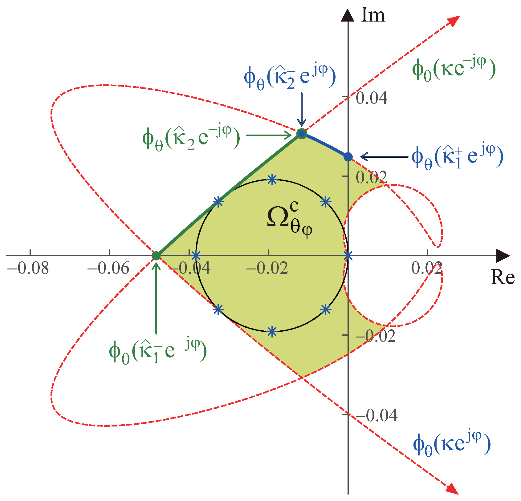
Once $\phi =23\pi /36$ [rad] was set, two domains, ${\Omega }_{{\theta }_{\phi }}$ and ${\Omega }_{{\theta }_{\phi }}^{\mathrm{c}}$, as defined in (18) in the complex plane, were derived using the image of ${\varphi }_{\theta }(\kappa e^{\pm j{\displaystyle \frac{23}{36}}\pi })$, where ${\varphi }_{\theta }\left(s\right)=s/g_{\theta }\left(s\right)$, as shown in Figure 8. As shown in Figure 8, two intervals of interest for $\kappa$ are $[{\widehat{\kappa }}_1^{+},{\widehat{\kappa }}_2^{+}]$ and $[{\widehat{\kappa }}_1^{-},{\widehat{\kappa }}_2^{-}]$, and ${\mathsf{\Gamma }}_{\pm }$ and ${\mathsf{\Psi }}_1^{\pm }$ defined by (27) and (28) accurately capture the situation. Under the system setting described above, ${\widehat{\kappa }}_1^{+}\approx 0.8252$, ${\widehat{\kappa }}_2^{+}\approx 1.1314$, ${\widehat{\kappa }}_1^{-}\approx 4.3031$, and ${\widehat{\kappa }}_2^{-}\approx 4.8041$. Thus, ${\lambda }_{c_1}^{+}={\displaystyle \frac{{\widehat{\kappa }}_1^{+}+{\widehat{\kappa }}_2^{+}}{2}}{e}^{j{\displaystyle \frac{23\pi }{36}}}=-4.1344+0.8866j$ and ${\lambda }_{c_1}^{-}={\displaystyle \frac{{\widehat{\kappa }}_1^{-}+{\widehat{\kappa }}_2^{-}}{2}}{e}^{-j{\displaystyle \frac{23\pi }{36}}}=-1.9244+4.1270j$.

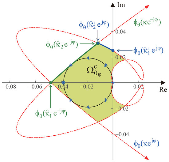
Figure 8. Image of ${\varphi }_{\theta }\left(\kappa e^{\pm j\varphi }\right)$ with $\varphi ={\displaystyle \frac{23}{36}}\pi$ and the eight poles of $A_{\theta }$ corresponding to $k_{\theta }=0.0191(\approx k_{{max}_{\theta }})$.

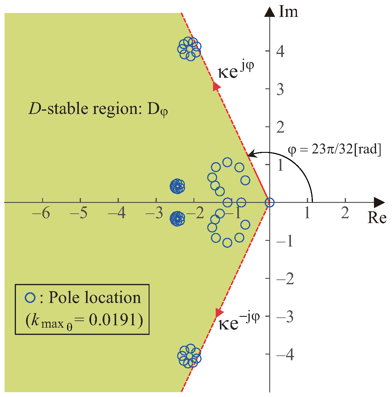
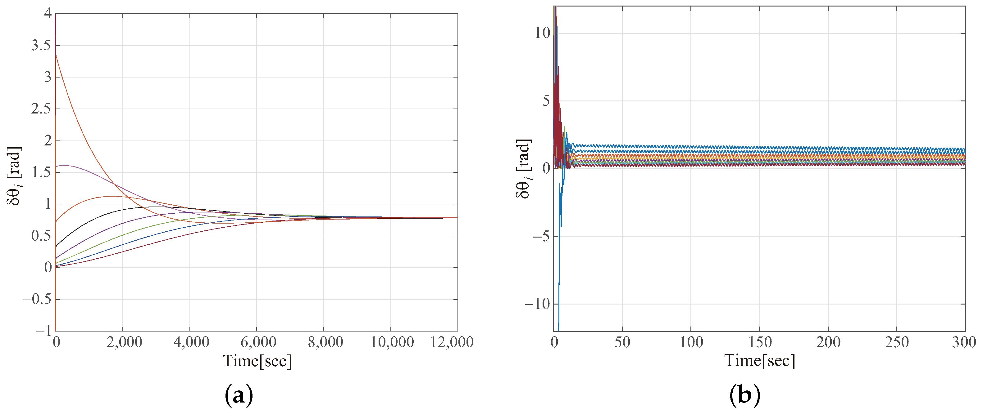
By solving the “Optimization problem for Problem S” in (29) of Section 4.2 using the MATLAB LMI add-on solver YALMIP (version 20230622) and MOSEK (version $10.0.38$), the upper bound $k_{{max}_{\theta }}$ of the connectivity gain $k_{\theta }(>0)$ was obtained as $k_{{max}_{\theta }}\approx 0.0191$. For $k_{\theta }=0.0191$, Figure 8 clearly shows that one of the eigenvalues of $A_{\theta }$ is at the origin of the complex plane, while the remaining seven eigenvalues lie within the domain ${\Omega }_{{\theta }_{\phi }}^{\mathrm{c}}$. Therefore, it can be infered from Proposition 1 that one of the poles of ${\mathcal{H}}_{\theta }\left(s\right)$ in (14) corresponding to $g_{\theta }\left(s\right)$ in (33) and $k_{\theta }=0.0191$ is at the origin of the complex plane, and the remaining poles lie within the $\mathcal{D}$-stable region ${\mathrm{D}}_{\phi }$, as confirmed from Figure 9. Further analysis is provided through experimental data to illustrate the dynamic behavior under different connectivity gains. Specifically, Figure 10a displays the time histories of $\delta {\theta }_i\left(t\right)$ for all eight agents with a connectivity gain of $k_{\theta }=0.0191$. This setup demonstrates effective $\mathcal{D}$-stablization, as each agent’s $\delta {\theta }_i\left(t\right)$ converges towards a stable state, showcasing the stabilization technique’s efficacy. In contrast, Figure 10b captures the behavior with a connectivity gain of $k_{\theta }=0.07 (>k_{{max}_{\theta }}\approx 0.0191)$, which does not achieve optimal $\mathcal{D}$-stablization. Here, the trajectories exhibit significant oscillatory behavior, which indicates continual adjustments in the relative angles between agents. Such persistent oscillations are generally undesirable in control systems, as they may lead to less predictable and less coordinated agent interactions. This approach makes it possible to easily obtain desirable time responses by simply solving the generalized KYP lemma-based LMI optimization problem with the appropriate set of matrices ${\mathsf{\Gamma }}_{\pm }$ and ${\mathsf{\Psi }}_1^{\pm }$. These simulation results underscore the efficacy and robustness of the proposed technique, demonstrating its potential as a powerful tool for addressing complex challenges in this field.

Figure 9. Poles of ${\mathcal{H}}_{\theta }\left(s\right)$ in (14) corresponding to $g_{\theta }\left(s\right)$ in (33) and $k_{\theta }=0.0191(\approx k_{{max}_{\theta }})$.

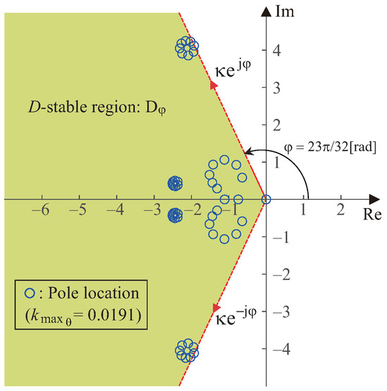
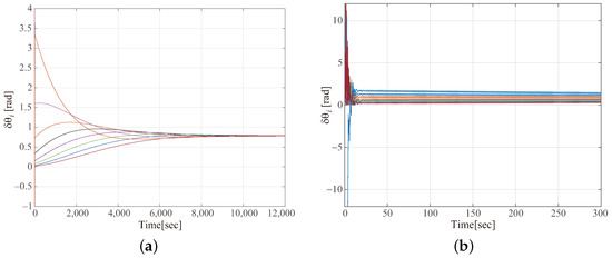
Figure 10. Comparative analysis of $\delta {\theta }_i\left(t\right)$ with connectivity gains of $k_{\theta }=0.0191$ and $k_{\theta }=0.07 (>k_{{max}_{\theta }}\approx 0.0191)$ for agents $i=1,2,\cdots ,8$. (a) Time history of $\delta {\theta }_i\left(t\right)$ for each agent with successful $\mathcal{D}$-stabilization using $k_{\theta }=0.0191$ and (b) Time history of $\delta {\theta }_i\left(t\right)$ for each agent without $\mathcal{D}$-stabilization using $k_{\theta }=0.07$.

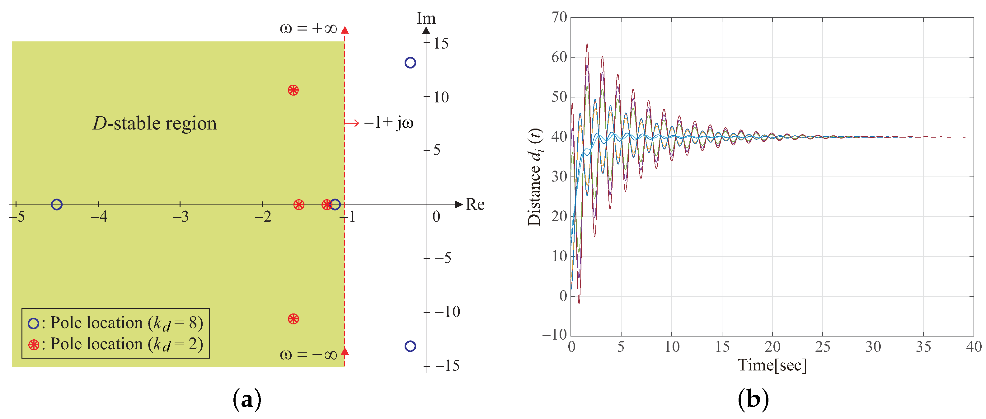
On the other hand, the d- or $\alpha$-directional $\mathcal{D}$-stabilization can be easily achieved compared to the $\theta$-directional stabilization problem, as mentioned at the end of Section 3, because $A_d$ in (11) and $A_{\alpha }$ in (12) have n multiple eigenvalues at $(-k_d+j0)$ and $(-k_{\alpha }+j0)$, respectively. For example, if the goal is to place all the poles of ${\mathcal{H}}_d\left(s\right)$ with $p_d\left(s\right)=1/\left(s(s-1)\right)$ and $c_d\left(s\right)=12\left(1+1/3s+s/4\right)$ in the predesignated $\mathcal{D}$-stable region shown in Figure 11a, then $(-k_d+j0)$ must belong to the domain ${\Omega }_D^{\mathrm{c}}$ defined as:

$$\begin{array}{c}{\Omega }_D:={\varphi }_d\left({\mathbb{C}}_D\right),{\Omega }_D^{\mathrm{c}}:=\mathbb{C}\backslash {\Omega }_D,\hfill \\ {\displaystyle {\varphi }_d\left(s\right)=\frac{\frac{1}{108}{s}^4+\frac{1}{18}{s}^3+s^2+s}{\frac{1}{12}{s}^2+s+1},}\hfill \end{array}$$

(34)

where ${\mathbb{C}}_D=\{s\in \mathbb{C}:\mathrm{Re}\left[\mathrm{s}\right]\ge -1\}$ (see Figure 12). Figure 11a demonstrates that while all the closed-loop poles for $k_d=2$ are located within the $\mathcal{D}$-stable region, represented by the shaded area, the poles for $k_d=8$ do not satisfy the $\mathcal{D}$-stability condition and are located outside this region. Additionally, Figure 11b illustrates the time histories of the distances $d_i\left(t\right)$ for each of the eight agents using $k_d=2$. This demonstrates how each trajectory eventually stabilizes at $D=40$, highlighting the dynamic and steady-state behaviors achieved under the defined $\mathcal{D}$-stabilization condition.

Figure 11. Stability and response analysis of closed-loop system ${\mathcal{H}}_d\left(s\right)$. (a) Pole positions at control settings $k_d=2$ within, and $k_d=8$ outside, the $\mathcal{D}$-stable region and (b) Time response of $d_i\left(t\right)$ for agents with $k_d=0.2$, confirming $\mathcal{D}$-stability.

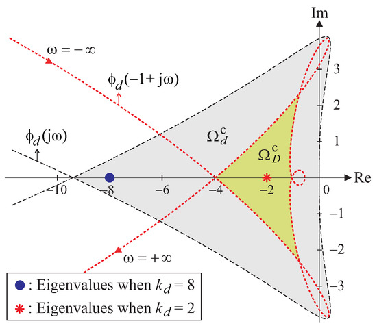
Figure 12. Image of ${\varphi }_d(-1+j\omega )$ and the corresponding domain ${\Omega }_D^c$.

Finally, to demonstrate the applicability of the $\mathcal{D}$-stabilization technique in more typical scenarios, consider the following 2nd-order $\theta$-directional dynamics $p_{\theta }\left(s\right)$:

$$p_{\theta }\left(s\right)={\displaystyle \frac{-4.202s^2-2.243s-4.21}{2.168s^2-3.332s+0.8577}}.$$

(35)

To stabilize this agent, a conventional PID controller $c_{\theta }\left(s\right)$ is introduced:

$$c_{\theta }\left(s\right)=2.538+{\displaystyle \frac{0.729}{s}}+1.211s.$$

(36)

Assuming a multi-agent system composed of seven agents, whose dynamics are represented by the stabilized $g_{\theta }\left(s\right)$, the $\mathcal{D}$-stable region is defined by $\phi =77\pi /120$ [rad] as shown in Figure 13a. Consequently, ${\varphi }_{\theta }\left(s\right)(={\displaystyle \frac{1}{h_{\theta }\left(s\right)}}={\displaystyle \frac{s}{g_{\theta }\left(s\right)}})$ and ${\Omega }_{{\theta }_{\phi }}^{\mathrm{c}}$ are derived as illustrated in Figure 14. The two intervals of interest for $\kappa$ are $[{\widehat{\kappa }}_1^{+},{\widehat{\kappa }}_2^{+}]$ and $[{\widehat{\kappa }}_3^{+},{\widehat{\kappa }}_4^{+}]$ where ${\widehat{\kappa }}_1^{+}\approx 0.3890$, ${\widehat{\kappa }}_2^{+}\approx 0.7790$, ${\widehat{\kappa }}_3^{+}\approx 1.3790$ and ${\widehat{\kappa }}_4^{+}\approx 1.4950$. Thus, ${\lambda }_{c_1}^{+}={\displaystyle \frac{{\widehat{\kappa }}_1^{+}+{\widehat{\kappa }}_2^{+}}{2}}{e}^{j{\displaystyle \frac{77\pi }{120}}}=-0.6165+1.2925j$ and ${\lambda }_{c_2}^{+}={\displaystyle \frac{{\widehat{\kappa }}_3^{+}+{\widehat{\kappa }}_4^{+}}{2}}{e}^{j{\displaystyle \frac{77\pi }{120}}}=-0.2514+-0.5271j$. By solving the “Optimization problem for Problem S” in Section 4.2 using the MATLAB LMI toolbox YALMIP (version 20230622) and MOSEK (version 10.0.38), the upper bound $k_{{max}_{\theta }}$ for the connectivity gain $k_{\theta }(>0)$ was obtained as approximately $0.17608$. For $k_{\theta }=0.17608$, Figure 13a clearly shows that, except for one pole located at the origin of the complex plane, all poles of ${\mathcal{H}}_{\theta }\left(s\right)$ reside within the $\mathcal{D}$-stable region ${\mathrm{D}}_{\phi }$. Moreover, Figure 13b vividly illustrates how each agent’s $\delta {\theta }_i\left(t\right)$ ($i=1,2,\cdots ,7$) converges to $2\pi /7\left[\mathrm{rad}\right]$ as $t\to \infty$. These insights confirm the effectiveness of the $\mathcal{D}$-stabilization technique across different system complexities, paving the way for future advancements in control strategies for multi-agent systems.

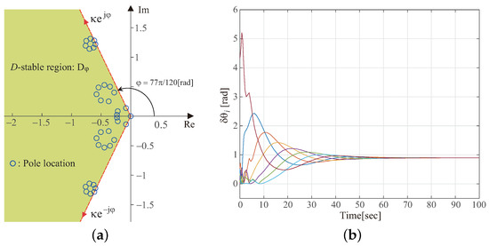
Figure 13. $\mathcal{D}$-stability and response analyses of closed-loop system ${\mathcal{H}}_{\theta }\left(s\right)$. (a) Pole locations of ${\mathcal{H}}_{\theta }\left(s\right)$ corresponding to $k_{\theta }=0.17608(\approx k_{{max}_{\theta }})$ and (b) Time history of $\delta {\theta }_i\left(t\right)$ for each agent when $k_{\theta }=0.17608$.

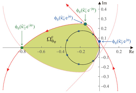
Figure 14. Image of ${\varphi }_{\theta }\left(\kappa e^{\pm j\varphi }\right)$ with $\phi ={\displaystyle \frac{77}{120}}\pi$ and the eight poles of $A_{\theta }$ corresponding to $k_{\theta }=0.17608(\approx k_{{max}_{\theta }})$.

Remark 1.

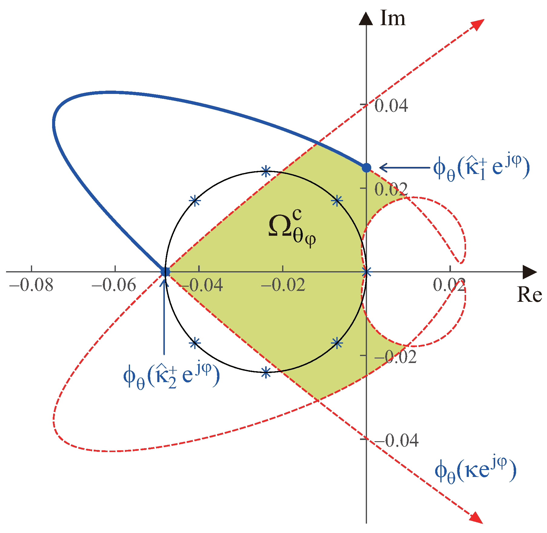
This study builds upon the research conducted in [28], in which one of the authors of this paper was a co-investigator. However, the study in [28] encountered several issues in the formulation of the “Optimization problem for Problem S” in Section 4.2, specifically in determining the upper bound $k_{{max}_{\theta }}$ of the connectivity gain $k_{\theta }(>0)$. The analysis in [28] did not adequately account for the various intervals of interest for κ corresponding to different ${\Omega }_{{\theta }_{\phi }}^{\mathrm{c}}$ cases, leading to an incomplete definition of both ${\mathsf{\Gamma }}_{\pm }$ and ${\mathsf{\Psi }}_1^{\pm }$, as described in (27) and (28). Furthermore, the constraint conditions in (25) and (26) were not precisely formulated. More specifically, the research in [28] assumed that since ${\varphi }_{\theta }\left(\kappa e^{j\phi }\right)$ and ${\varphi }_{\theta }\left(\kappa e^{-j\phi }\right)$ are symmetric about the real axis, considering only ${\varphi }_{\theta }\left(\kappa e^{j\phi }\right)$ would suffice to define the boundary of ${\Omega }_{{\theta }_{\phi }}^{\mathrm{c}}$ and thus determine the interval of interest for κ. As a result, the optimization problem in [28] focused on solving for a specific region of ${\varphi }_{\theta }\left(\kappa e^{j\phi }\right)$ bounded by $[{\widehat{\kappa }}_1^{+},{\widehat{\kappa }}_2^{+}]=[0.8252,4.3031]$ as shown in Figure 15. However, this approach neglected a portion of the boundary of ${\Omega }_{{\theta }_{\phi }}^{\mathrm{c}}$ that should have been included in the optimization process. Consequently, following the method in [28], the optimization yields a result of $k_{{max}_{\theta }}\approx 0.02403$, as illustrated in Figure 15, where two pairs of eigenvalues of $A_{\theta }$ fall outside the ${\Omega }_{{\theta }_{\phi }}^{\mathrm{c}}$ region. Based on Proposition 1, this implies that some poles of $\mathcal{H}\theta \left(s\right)$ do not lie within the desired $\mathcal{D}$-stable region $\mathrm{D}\phi$. This study addresses the errors and limitations of the optimization problem formulation in [28], providing a corrected approach that accurately determines the upper bound $k_{{max}_{\theta }}$ of the connectivity gain $k_{\theta }$(>0). This correction ensures that distributed coordination stabilization for all dynamic multi-agent systems is achieved.

Figure 15. Image of ${\varphi }_{\theta }\left(\kappa e^{j\varphi }\right)$ with $\varphi ={\displaystyle \frac{23}{36}}\pi$ and the eight poles of $A_{\theta }$ corresponding to $k_{\theta }=0.02403(\approx k_{{max}_{\theta }})$.

6. Conclusions

This study presented a novel formation $\mathcal{D}$-stabilization scheme for distributed cooperative control based on a cyclic pursuit strategy. A Lyapunov $\mathcal{D}$-stability problem in multi-agent dynamical systems was first introduced to systematically address convergence performance. Subsequently, a simple diagrammatic pursuit formation Lyapunov $\mathcal{D}$-stability criterion was developed. The challenge of maximizing the connectivity gain of a cyclic pursuit-based online path generator was shown to be reducible to an LMI optimization problem using the generalized GKYP lemma. Then, to clarify its distinctive features, we investigate the special case of the pursuit formation stabilization scheme for a class of multi-agent systems. To further elucidate its distinctive features, two cases of the pursuit formation stabilization scheme for a class of multi-agent systems were examined, through which the effectiveness of the proposed stabilization scheme was validated with numerical design examples.

References

- Liu, Y.; Liu, J.; He, Z.; Li, Z.; Zhang, Q.; Ding, Z. A survey of multi-agent systems on distributed formation control. Unmanned Syst. 2024, 12, 913–926. [Google Scholar] [CrossRef]
- Khan, A.; Niazi, A.U.K.; Raza, H.; Abbasi, W.; Awan, F. Resilient based consensus of fractional-order delayed multi-agent systems in Riemann-Liouville sense. Alex. Eng. J. 2023, 80, 348–357. [Google Scholar] [CrossRef]
- Amirkhani, A.; Barshooi, A.H. Consensus in multi-agent systems: A review. Artif. Intell. Rev. 2022, 55, 3897–3935. [Google Scholar] [CrossRef]
- Li, J.; Chen, S.; Li, C.; Wang, F. Distributed game strategy for formation flying of multiple spacecraft with disturbance rejection. IEEE Trans. Aerosp. Electron. Syst. 2021, 57, 119–128. [Google Scholar] [CrossRef]
- Liu, H.; Shao, X.; Liu, J.; Zhang, Q.; Li, X. Path-following formation coordination for multiple UAVs considering communication constraints. IEEE Trans. Aerosp. Electron. Syst. 2024, 9, 3436–3449. [Google Scholar] [CrossRef]
- Litimein, H.; Huang, Z.-Y.; Hamza, A. A survey on techniques in the circular formation of multi-agent systems. Electronics 2021, 10, 2959. [Google Scholar] [CrossRef]
- Yang, H.; Wang, Y. Cyclic pursuit-fuzzy PD control method for multi-agent formation control in 3D space. Int. J. Fuzzy Syst. 2021, 23, 1904–1913. [Google Scholar] [CrossRef]
- Peng, X.; Guo, K.; Geng, Z. Moving target circular formation control of multiple non-holonomic vehicles without global position measurements. IEEE Trans. Circuits Syst. II-Express Briefs 2020, 67, 310–314. [Google Scholar] [CrossRef]
- Xu, P.; Li, W.; Tao, J.; Dehmer, M.; Emmert-Streib, F.; Xie, G.; Xu, M.; Zhou, Q. Distributed event-triggered circular formation control for multiple anonymous mobile robots with order preservation and obstacle avoidance. IEEE Access 2020, 8, 167288–167299. [Google Scholar] [CrossRef]
- Shao, J.; Tian, Y.-P. Multi-target localisation and circumnavigation by a multi-agent system with bearing measurements in 2D space. Int. J. Syst. Sci. 2018, 49, 15–26. [Google Scholar] [CrossRef]
- Freitas, V.L.; Macau, E.E. Collision avoidance mechanism for symmetric circular formations of unitary mass autonomous vehicles at constant speed. Math. Probl. Eng. 2018, 2018, 6291082. [Google Scholar] [CrossRef]
- Miao, Z.; Wang, Y.; Fierro, R. Cooperative circumnavigation of a moving target with multiple nonholonomic robots using backstepping design. Syst. Control Lett. 2017, 103, 58–65. [Google Scholar] [CrossRef]
- Daingade, S.; Sinha, A.; Borkar, A.V.; Arya, H. A variant of cyclic pursuit for target tracking applications: Theory and implementation. Auton. Robot. 2016, 40, 669–686. [Google Scholar] [CrossRef]
- Mukherjee, D.; Ghose, D. Generalized hierarchical cyclic pursuit. Automatica 2016, 71, 318–323. [Google Scholar] [CrossRef]
- Juang, J.-C. On the formation patterns under generalized cyclic pursuit. IEEE Trans. Autom. Control 2013, 58, 2401–2405. [Google Scholar] [CrossRef]
- Ramirez-Riberos, J.L.; Pavone, M.; Frazzoli, E.; Miller, D.W. Distributed control of spacecraft formations via cyclic pursuit: Theory and experiments. J. Guid. Control Dyn. 2010, 33, 1655–1669. [Google Scholar] [CrossRef]
- Wang, Q.; Lv, Y.; Wang, Q.; Duan, Z.; Chen, G. Distributed consensus of multiagent systems: An integrated adaptive approach. IEEE Trans. Netw. Sci. Eng. 2024, 11, 3550–3562. [Google Scholar] [CrossRef]
- Shao, X.; Li, S.; Zhang, J.; Zhang, F.; Zhang, W.; Zhang, Q. GPS-free collaborative elliptical circumnavigation control for multiple non-holonomic vehicles. IEEE Trans. Intell. Veh. 2023, 8, 3750–3761. [Google Scholar] [CrossRef]
- Peng, X.; Yi, R.; Wang, P.; Lv, Y. Circular formation control of target enclosing for fixed-wing UAVs in three-dimensional space. IEEE Trans. Intell. Veh. 2024, 1–11. [Google Scholar] [CrossRef]
- Kim, T.-H.; Sugie, T. Cooperative control for target-capturing task based on a cyclic pursuit strategy. Automatica 2007, 43, 1426–1431. [Google Scholar] [CrossRef]
- Kwak, T.; Kim, Y.; Hori, Y.; Kim, T.-H. Graphical and analytical approaches for analyzing collective behavior of dynamic multi-agent systems governed by generalized cyclic pursuit mechanism. IEEE Access 2023, 11, 140481–140495. [Google Scholar] [CrossRef]
- Kim, T.-H.; Hara, S.; Hori, Y. Cooperative control of multi-agent dynamical systems in target-enclosing operations using cyclic pursuit strategy. Int. J. Control 2010, 83, 2040–2052. [Google Scholar] [CrossRef]
- Hara, S.; Hayakawa, T.; Sugata, H. Stability analysis of linear systems with generalized frequency variables and its application to formation control. In Proceedings of the 46th IEEE Conference on Decision and Control, New Orleans, LA, USA, 12–14 December 2007; pp. 1459–1466. [Google Scholar]
- Hara, S.; Hayakawa, T.; Sugata, H. LTI systems with generalized frequency variables: A unified framework for homogeneous multi-agent dynamical systems. SICE J. Control. Meas. Syst. Integr. 2009, 2, 299–306. [Google Scholar] [CrossRef]
- Tanaka, H.; Hara, S.; Iwasaki, T. LMI stability condition for linear systems with generalized frequency variables. In Proceedings of the 2009 7th Asian Control Conference, Hong Kong, China, 27–29 August 2009; pp. 136–141. [Google Scholar]
- Hara, S.; Iwasaki, T.; Shiokata, D. Robust PID control using generalized KYP synthesis: Direct open-loop shaping in multiple frequency ranges. IEEE Control Syst. Mag. 2006, 26, 80–91. [Google Scholar]
- Iwasaki, T.; Hara, S. Generalized KYP lemma: Unified frequency domain inequalities with design applications. IEEE Trans. Autom. Control 2005, 50, 41–59. [Google Scholar] [CrossRef]
- Kim, T.-H.; Hara, S. Stabilization of multi-agent dynamical systems for cyclic pursuit behavior. In Proceedings of the 2008 47th IEEE Conference on Decision and Control, Cancun, Mexico, 9–11 December 2008; pp. 4370–4375. [Google Scholar]
Disclaimer/Publisher’s Note: The statements, opinions and data contained in all publications are solely those of the individual author(s) and contributor(s) and not of MDPI and/or the editor(s). MDPI and/or the editor(s) disclaim responsibility for any injury to people or property resulting from any ideas, methods, instructions or products referred to in the content. |
© 2024 by the authors. Licensee MDPI, Basel, Switzerland. This article is an open access article distributed under the terms and conditions of the Creative Commons Attribution (CC BY) license (https://creativecommons.org/licenses/by/4.0/).