Abstract
This paper proposes an incremental nonlinear control method for an aeroelastic system’s gust load alleviation and active flutter suppression. These two control objectives can be achieved without modifying the control architecture or the control parameters. The proposed method has guaranteed stability in the Lyapunov sense and also has robustness against external disturbances and model mismatches. The effectiveness of this control method is validated by wind tunnel tests of an active aeroelastic parametric wing apparatus, which is a typical wing section containing heave, pitch, flap, and spoiler degrees of freedom. Wind tunnel experiment results show that the proposed nonlinear incremental control can reduce the maximum gust loads by up to 46.7% and the root mean square of gust loads by up to 72.9%, while expanding the flutter margin by up to 15.9%.
1. Introduction
Modern transport aircraft commonly feature high-aspect-ratio wings to increase aerodynamic efficiency. A disadvantage of increasing the wing aspect ratio is the increased susceptibility to gust and manoeuvre loads in addition to the onset of aeroelastic phenomena such as flutter and divergence. In the literature, there are typically two approaches to alleviate gust loads and suppress flutter: passive aeroelastic tailoring and active control [1]. The passive approach has a long history and is achieved by exploiting the anisotropic properties of composite material to steer dynamic and static aeroelastic behaviour. By contrast, the active approach designs feedforward and/or feedback controllers to actuate the leading-edge and/or trailing-edge control surfaces for load redistribution and closed-loop dynamic modification. This paper focuses on the active approach because typically, it has a better adaptability to variations in flight and load conditions than its passive counterpart [1].
The majority of active gust load alleviation (GLA) and flutter suppression control algorithms are designed based on a reduced-order, linear, time-invariant state-space aero(servo)elastic model. These algorithms include proportional–integral–derivative control [2], pole placement [3], linear quadratic regulator/Gaussian [4], eigensystem synthesis, analysis [5], and linear robust control ( and [6]). Although these linear control approaches have shown their effectiveness in practice, the resulting controllers only have a guaranteed stability and performance around the linearization point; thus, the additional and tedious gain-scheduling method [7] is required to expand these linear controllers to a wider flight envelope. Furthermore, it is challenging for linear controllers to passively tolerate some specific nonlinearities (i.e., free-play, backlash hysteresis [8], bifurcation [9]), sudden faults in actuators and/or sensors, and structure damage.
On the contrary, nonlinear control methods, especially those that have guaranteed stability in the Lyapunov sense, have shown great potential in solving nonlinear aeroservoelastic system control problems without requiring the gain-scheduling technique. An immersion and invariance controller was proposed in [10] for nonlinear flutter suppression and free-play compensation. Platanitis et al. [11] used the nonlinear dynamic inversion approach together with the model reference adaptive control technique for the limit cycle oscillation suppression of a typical aeroelastic wing section. Recurrent neural networks have been used for nonlinear model identification and active flutter suppression in [12]. However, these nonlinear control approaches have a relatively high model dependency, while offline and/or online model identification of a nonlinear aeroservoelastic system is a nontrivial task. When sudden faults occur during flight, the convergence rate of online model identification can be insufficient to guarantee stability.
Different from model-based nonlinear control methods in the literature, the incremental nonlinear dynamic inversion (INDI) control is a sensor-based approach [13]. It is derived from nonlinear dynamic inversion (NDI) or feedback linearization, which linearizes the input–output mapping of a nonlinear system via feedback, resulting in a chain of integrators that can be easily stabilized by a linear virtual control [13]. The INDI method inherits the merits of NDI. More importantly, it greatly reduces the model dependency of NDI via exploiting sensor measurement [13]. In conventional NDI, since a perfect model is never known and external disturbances always exist in reality, the ideal linearization never exists, leading to robustness issues. By contrast, INDI makes full use of sensing information and simultaneously reduces the model dependency and improves control robustness. In the literature, INDI has been applied to a free-flying flexible aircraft tracking problem [14] and a morphing-wing gust load alleviation problem [15]. However, the effectiveness of INDI on flutter suppression, especially in a real-world environment, remains to be proven.
In this paper, we propose to use the sensor-based incremental nonlinear dynamic inversion control to tackle the active gust load alleviation and flutter suppression problems of an aeroservoelastic system. The goal is to use one single controller to simultaneously achieve these two objectives without requiring a gain adjustment, control architecture variations, or gain scheduling. The reduced model-dependency of INDI also reduces its practical implementation effort. The performance, robustness, and implementation ease of the proposed control method are validated by wind tunnel experiments on our newly developed active, aeroelastic, parametric wing apparatus.
2. Methods
2.1. Dynamic Model for a Typical Aeroelastic Wing Section
The equations of motion for a typical aeroelastic wing section can be written as [16]
where h is the vertical displacement or plunge of the airfoil; is the pitch angle of the wing section; is the deflection angle of the control surface; m is the mass per unit length of the wing section; S is the static mass moment of the wing around the pitch axis; is its mass moment of inertial around the same axis; the static mass moment of the control surface around the hinge axis is denoted by ; is the moment of inertia of the control surface around the hinge axis; is the product of inertia; denote the extension spring’s stiffness, the torsional spring’s stiffness related to , and the torsional spring’s stiffness related to , respectively; is the lift; is the pitching moment of the wing section around the pitch axis; and is the pitching moment of the control surface around the hinge axis. We assume structural damping is negligible, which is a common assumption in the field. An illustration of a typical aeroelastic wing section is show in Figure 1.
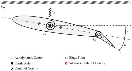
Figure 1.
An illustration of a typical aeroelastic wing section.
Theodorsen’s unsteady aerodynamic theory was adopted [16]. We indicate the half-chord length as b. Using the exponential approximation of Wagner’s function with , , , and [16], we obtain the complete equations of motion for a pitch–plunge airfoil with control surface as
where and represents the aerodynamic lag states, is the density of the flow, U is the speed of the flow. The detailed expressions of the matrices can be derived from Equation (1) and can also be found in [16]. The external lift and moments in Equation (2) are gusts- and control-surface-deflection-induced components of the total lift and moments in Equation (1).
The loads due to a gust are represented as , in which the lift is a purely circulatory event. The gust velocity is implemented in circulatory lift calculations with the Küssner function. The Küssner function is approximated with exponential form with , , , and . Denote the gust input velocity as ; denote and as the aerodynamic lag states due to gust; then, we have
After applying the Leibnitz integration rule and using the Küssner function, the complete expressions for the aerodynamic loads due to a gust are defined as:
where the parameter a and are defined as in [16].
Assume that the inertial coupling force/moment for the control surface with regard to the rest of the wing section are negligible; then, the independent servo actuator dynamics is governed by
where is the control command for the aileron, and the coefficients are obtained using the system identification of the servo.
Then, the dynamics for state is governed by
where and are the corresponding matrices for fragmented from Equation (2).
The resulting external force and moment due to the control surface deflection are modelled as
where
and and to are defined as in [16].
Ignoring the inertia coupling between the aileron actuator and the rest of the wing section and substituting Equation (5) into Equation (7), we have
Now, choose state , control output , and control input . The following control-oriented state-space model is obtained:
where
with
2.2. Incremental Nonlinear Dynamic Inversion
The incremental nonlinear dynamic inversion (INDI) method can control the following nonlinear system:
where and are smooth vector fields. is a smooth function mapping , whose columns are smooth vector fields. The external disturbance vector is , which is assumed to satisfy . The external disturbances in the real world can easily satisfy this boundedness assumption.
In Equation (13), denotes the controlled output vector. This paper considers the case where , which means the system is either fully actuated or overactuated. The vector relative degree [17] of the system is defined as , which satisfies . From Equation (13), the input–output mapping of the nonlinear system is
In Equation (14), , , and , where are the corresponding Lie derivatives [18]. When for all , . When , the system given by Equation (13) is full-state feedback linearizable. Otherwise, internal dynamics exist.
INDI considers system variations in one sampling interval . The incremental dynamic equation is derived by taking the first-order Taylor series expansion of Equation (14) around the condition at (denoted by the subscript 0) as:
in which , , and represent the state, control, and disturbance increments in one sampling time step , respectively. is the expansion remainder. Define the internal state vector as and the external state vector as , , . In a stabilization problem, the reference for the controlled output equals zero and the control increment is designed to satisfy
where is an estimation of . The gain matrix , and . can be directly measured or estimated. The total control command for the actuator is , in which can be measured or estimated using an actuator model. Considering the internal dynamics, the resulting closed-loop dynamics are:
where is a diffeomorphism. The term is the closed-loop value of the variations and expansion reminder:
, , , , and is the canonical form representation of a chain of integrators. The gain matrix is designed to guarantee that is Hurwitz [13].
Theorem 1.
If is satisfied for all , is continuously differentiable and globally Lipschitz in , and the origin of is globally exponentially stable, then the external state ξ in Equation (17) is globally ultimately bounded by a class function of , while the internal state η in Equation (17) is globally ultimately bounded by a class function of and .
Proof .
This can be proved by applying Theorem 1 in Ref. [15] and setting the reference vector to zero. □
Theorem 2.
If is satisfied for all , is continuously differentiable, and the origin of is exponentially stable, then there exists a neighborhood of and , such that for every initial state and , the external state ξ in Equation (17) is ultimately bounded by a class function of , while the internal state η in Equation (17) is ultimately bounded by a class function of and .
Proof .
This can be proved by applying Theorem 2 in Ref. [15] and setting the reference vector to zero.
Theorems 1 and 2 prove that under the perturbation of bounded uncertainties and disturbances and with stable internal dynamics, the closed-loop system under INDI control is stable in the Lyapunov sense. □
2.3. INDI Design for an Aeroelastic Wing
In this research, we focused on stabilizing the heave degree of freedom of an aeroelastic wing using the trailing-edge flap. Consequently, in Equation (9), the controlled output is h, while the input . This leads to an input–output mapping with a relative degree equal to two. Applying Equation (16), the aileron’s input for stabilization is designed as:
where and are differential and proportional gains. The aileron’s control input command equals , in which is the control input at the previous time point.
In Section 3, we validate the performance of the INDI method for gust load alleviation and active flutter suppression challenges. It is noteworthy that this single controller can solve both issues without changing the control architecture or the control gains. A control and block diagram is presented in Figure 2.
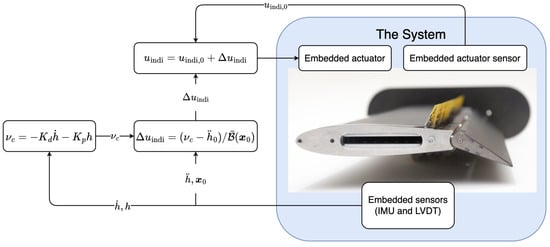
Figure 2.
Control and implementation block diagram.
3. Experiment Setup
The proposed controller for active gust load alleviation and flutter suppression was validated using an aeroelastic wing apparatus by wind-tunnel testing. The self-designed active wing section [19] itself was mounted in an aeroelastic apparatus (AA) developed by Gjerek et al. [20]. The AA consisted of a rectangular, acrylic section mounted on the gust generator and providing heave and pitch degrees of freedom, with adjustable stiffness. In addition to the adjustable stiffness, weights can be added forward or rearward of the pitch axis, allowing both the mass distribution of the wing to be easily changed. The wing section was equipped with a movable full-span trailing-edge control surface (aileron) and a spoiler, which were actuated by high-bandwidth, electric servo actuators. The main focus of this experiment was to use the aileron for controlling the heave degree of freedom. The wing was also equipped with an MPU-9250 inertial measurement unit (IMU), as well as linear and rotation variable differential transformers (LVDT-Sentech 75DC-500/RVDT-Midori QP-2HC) for the measurements of acceleration, angular rates, heave, and pitch. All combined, this AA provided a setup that closely resembled the typical section, a two-dimensional wing section with an aileron and heave and pitch degrees of freedom (DOFs), in combination with the aerodynamic model developed by Theodorsen [21], which was presented in Section 2.1.
Wind tunnel testing was performed at the low-speed W-tunnel at Delft University of Technology, which is an open-circuit blow-down tunnel with a 0.4 m × 0.4 m test section, with low turbulence levels and a maximum attainable speed of 35 m/s. Attached to the wind tunnel is a gust generator capable of generating sinusoidal and cosine gust excitations with gust frequencies ranging from 0.5 Hz to 12 Hz in 0.5 Hz increments [22]. The aeroelastic apparatus in the wind tunnel is shown in Figure 3.
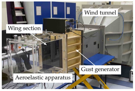
Figure 3.
Wind tunnel with the gust generator and aeroelastic apparatus.
The heave DOF was provided by two pairs of cantilever leaf springs, with one end of the springs clamped to the AA and the other end connected to a pitch assembly. The axles protruding from both sides of the wing were connected to bearings in the pitch assembly. The length of the leaf springs could be changed, providing a variable spring stiffness in the heave. Torsional stiffness was provided by a pair of axial springs connected to one of the axles by a pulley. The torsional stiffness could be varied by changing the diameter of the pulley or exchanging the axial springs. A top view of the AA is seen in Figure 4, showing the top half of the heave and pitch mechanism.
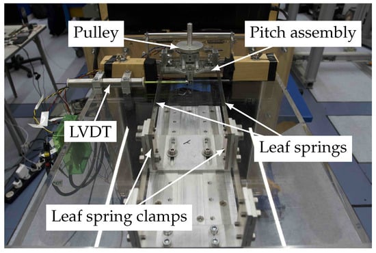
Figure 4.
Top view of the aeroelastic apparatus. Note, the RVDT is placed on the bottom side.
The specifications of the aeroelastic wing apparatus for GLA and flutter suppression are shown in Table 1. When the blades of gust generator deflected at a certain frequency, gusts were generated in the wing section test field with a gust-induced angle of attack , where is the initial time, is the amplitude of the blades’ deflection angle, and is the gust coefficient relevant to the velocity U and the gust generator frequency . A second-order model for the aileron’s actuation mechanism was given by . The minimal and maximal deflections were limited to and , and the maximum deflection rate was estimated to be 750/s. The IMU used on the apparatus had a bandwidth of 200 Hz. The LVDT had a cut-off frequency of 200 Hz and was read by a 12-bit analogue-to-digital converter, resulting in a resolution of approximately 6 × 10 mm. The sampling interval was set as 0.002 s for capturing the high-frequency aeroelastic modes. The measured outputs used by the controller were the heave acceleration from the IMU, the heave displacement h from the LVDT, and the control surface deflection .

Table 1.
Configuration parameters of the aeroelastic apparatus.
4. Results and Discussion
In this section, the experimental results are discussed. First, the GLA results are presented in Section 4.1. Then, this is followed by the flutter suppression results in Section 4.2.
4.1. Gust Load Alleviation Results
The GLA results are presented in this subsection. In the wind tunnel test, and were chosen for the controller gains based on the desired eigenvalues of the closed-loop system. The nominal control effectiveness for 12 m/s was identified from a wind tunnel test as . The open- and closed-loop experiments were performed for gust frequencies of 3, 3.5, 4, 4.5, and 5 Hz, and a gust amplitude of . In addition to the directly measured outputs and h from the IMU and LVDT, a Luenberger observer with eigenvalues was applied to provide an estimation of by using the measurements of the heave displacement and acceleration. was required for the implementation of the control law as shown in Equation (19). An overview of the measured and estimated signals is shown in Figure 5.
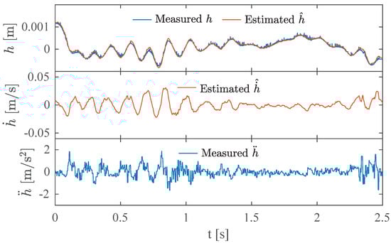
Figure 5.
Overview of the measured and estimated signals.
For the GLA experiments, the wing was subjected to a series of cosine gusts. First, the open-loop gust response was determined, after which the experiment was repeated with the controller enabled. Figure 6, Figure 7 and Figure 8 show the recorded GLA data for gust frequencies of 3, 4, and 5 Hz. The results show significant improvements in reducing the amplitude of h. The top plot of each subfigures shows the theoretical gust input in terms of the gust-induced angle of attack . At each frequency, the experiments were repeated four times to evaluate the coherence of the results.
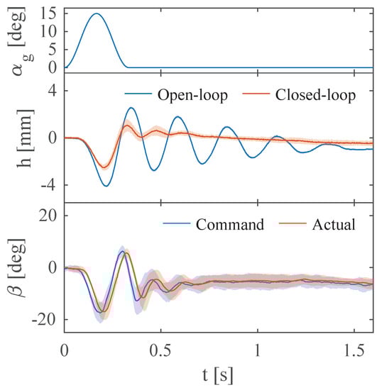
Figure 6.
The heave displacement comparisons between open- and closed-loop gust responses when the gust frequency Hz. is the gust’s input angle while is the control surface’s reflection angle.
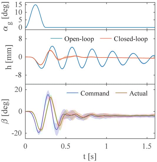
Figure 7.
The heave displacement comparisons between open- and closed-loop gust responses when the gust frequency Hz. is the gust’s input angle while is the control surface’s reflection angle.
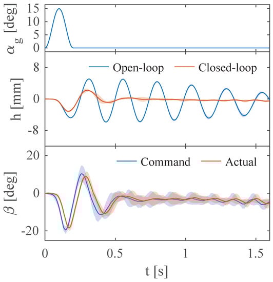
Figure 8.
The heave displacement comparisons between open- and closed-loop gust responses when the gust frequency Hz. is the gust’s input angle while is the control surface’s reflection angle.
The middle subplots show comparisons of the mean values of the open-loop (dashed line) and closed-loop responses (solid line). Also included in each middle subplot is the standard deviation of the heave response as a shaded region, which nearly coincides with the mean data, proving the coherence and repeatability of the experimental results. The transient, open-loop heave response in the middle plots can be subdivided into two parts. During the first half-period of the oscillation, the response is dominated by the gust input. For the remainder of the transient response, the wing oscillates with a frequency of approximately 4 Hz, close to the frequency of the first heave mode of the wing section. Whereas the open-loop results are highly underdamped, the closed-loop responses are mostly damped out after one full period.
The commanded and actual aileron deflections are detailed in the bottom subplots of Figure 6, Figure 7 and Figure 8. It can be observed that the aileron is settled on a steady-state deflection after the convergence of the heave response. Results from Schildkamp et al. [19] show the magnitude and phase responses of the servo actuator degrades for frequencies higher than 2 Hz. Since the servo actuator is now connected to the aileron, adding inertia and friction to the system, the frequency response is expected to be worse than what was presented in [19]. The commanded aileron deflection has a frequency similar to that of the heave response, explaining the differences in magnitude and phase between the commanded and actual aileron deflection. The larger variability seen in both aileron deflection signals is attributed to noise in the signals driving the controller. The excitation frequency of 5 Hz is close to the pitch mode natural frequency of 6.39 Hz. Since this study focused on the heave motion, the uncontrolled pitch motion inertially coupled with the control surface’s movement, leading to the high frequency and low magnitude oscillations in control deflections in Figure 8, although the steady-state oscillations in heave were damped out.
A summary of the GLA results in terms of the reduction of the absolute peak value and RMS heave values for all previously mentioned gust frequencies is shown in Table 2, where the absolute peak heave value relates to the peak load endured by the wing, and the RMS value gives a measure of the vibrational loads the wing endures, related to the fatigue life of a structure. The mean, minimum, and maximum reduction rates for both the absolute peak and RMS values are given. Overall, the proposed INDI control method, without adjusting control gains, provides an attenuation higher than for the vibration amplitude due to a gust disturbance, and an attenuation higher than for the RMS(h). The greatest reduction in absolute peak and RMS mean values are achieved for a gust frequency of 5 Hz, with values of 71.4 and 44.2%, respectively. Previous results show the overall lowest damping coefficient for the open-loop gust response at 5 Hz, giving the highest RMS value. The controller quickly damps out the gust-induced oscillations, leading to the second-lowest closed-loop RMS value, hence the greatest reduction in RMS. Similarly, this is also the case for the absolute peak value, with the highest open-loop peak value and the second lowest peak value.
Table 2.
GLA controller reduction rate of the heave displacement h.
In addition to the open- and closed-loop heave responses plotted in the time domain, Figure 9 shows the power spectral density (PSD) of these heave responses in the frequency domain for gust frequencies of 3, 4, and 5 Hz. Also indicated in this figure are the (1) first heave mode, (2) first pitch mode, and (3) first rocking mode at 3.55, 6.39, and 11.10 Hz, respectively, as identified using a ground vibration test (GVT) described in [19]. The open-loop response results in two distinct peaks, around 4 and 12 Hz, at frequencies slightly higher than the first heave and rocking modes. Changes to the hardware and wiring of the wing section were made after the GVT, likely affecting the identified frequencies. This will be verified during a future GVT.
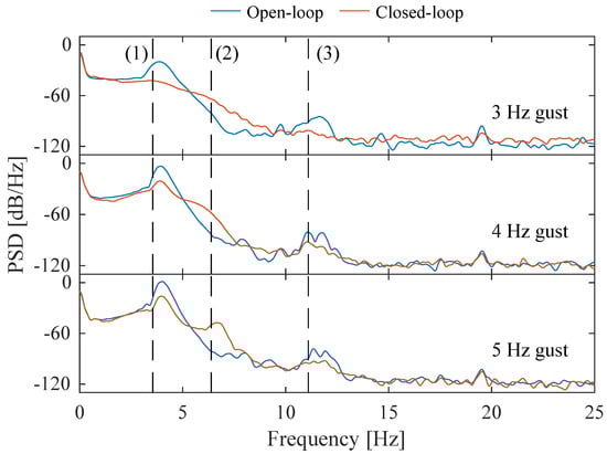
Figure 9.
A comparison between the open- and closed-loop gust responses’ power spectral density when the gust frequencies are 3, 4, and 5 Hz.
Three observations can be made from the closed-loop PSDs. First, as expected, the energy near the heave and rocking modes is reduced as the heave motion is primarily influenced by the use of the controller. Secondly, an increase in energy can be seen near the first pitch mode. This result is also expected, as the implemented controller does not directly damp out the pitch mode, and it is well-known that if a trailing-edge control device is used for GLA, then the root bending moment is alleviated at the expense of the amplification in the root torsional moment [23]. Furthermore, deflecting the aileron not only induces a heave motion but also a pitching motion around the elastic axis. Finally, no differences can be observed for frequencies greater than 15 Hz owing to the finite actuator bandwidth.
4.2. Flutter Suppression Results
In this subsection, we evaluated the flutter suppression ability of the INDI controller designed in Equation (19). Both the control architecture and control gains () were kept the same as in the GLA experiment. It is noteworthy that the control effectiveness is a function of dynamic pressure. Therefore, it was scaled by during the experiment. The static flow velocity U was known and was converted from the tunnel’s RPM value. The open-loop flutter speed was determined to be using the parametric flutter margin method [19]. Moreover, the control reversal speed was also determined for this configuration as m/s, which was slightly below the flutter speed.
To test the performance of the controller for flutter suppression, the flow velocity was gradually increased in steps past the flutter speed up to a velocity of 18.5 m/s. At each velocity step, the wing section was excited from its equilibrium position to trigger flutter. For consistent excitations of the wing section, it was subjected to a predefined cosine gust. First, open-loop flutter was recorded. To prevent any damage to the wing section or test setup, the wing section was manually stopped and returned to its equilibrium position after flutter occurred. The manual stopping of the wing was visible in the plotted gust responses by clipping and sharp peaks in the heave responses seen in Figure 10 and Figure 11. After recording the open-loop flutter, the controller was activated, and the wing section was excited again to record the closed-loop flutter response.
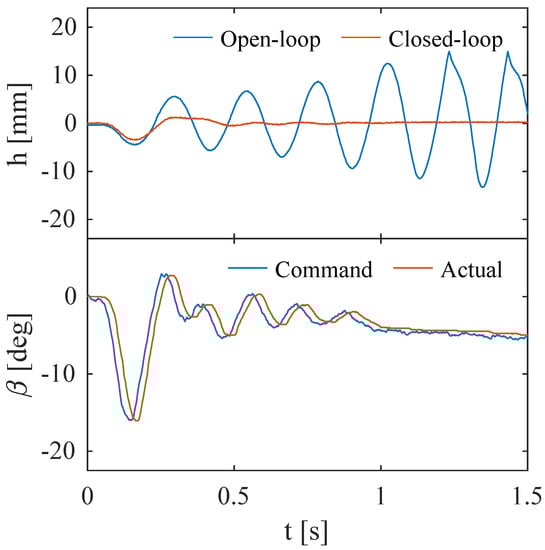
Figure 10.
Flutter suppression and gust response alleviation effectiveness when the flow velocity m/s.
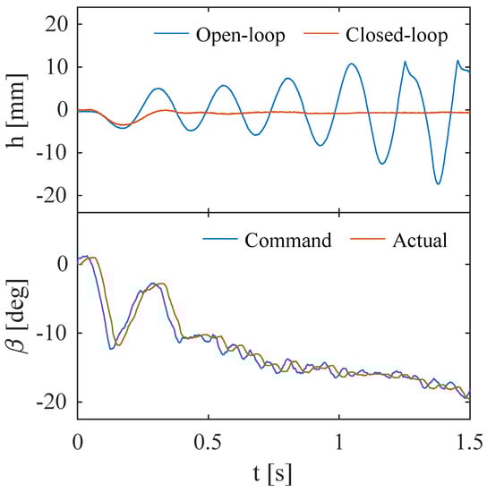
Figure 11.
Flutter suppression and gust response alleviation effectiveness when the flow velocity m/s.
Figure 10, Figure 11, Figure 12 and Figure 13 show a comparison of the open- and closed-loop heave response and the commanded and actual aileron deflection for the closed-loop response for increasing flow velocities past the open-loop flutter velocity. All open-loop responses to the excitation start with a 5 mm amplitude and expectedly oscillate with a frequency around 4 Hz, again close to the first heave mode. Figure 10 and Figure 11 show a clear diverging open-loop response. The closed-loop responses show the reduction of the heave response to the initial excitation compared to the open-loop response, after which the disturbance is damped out within approximately one period.
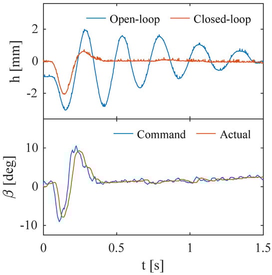
Figure 12.
Flutter suppression and gust response alleviation effectiveness when the flow velocity m/s.
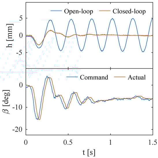
Figure 13.
Flutter suppression and gust response alleviation effectiveness when the flow velocity m/s.
Similar to the GLA results, the actual aileron deflection shows a slight lag in time of 0.02 s. For the higher velocities, Figure 10 and Figure 11, a nonzero aileron deflection can be observed after the initial disturbance has been damped out. Since the test conditions are beyond the control reversal speed, the heave response, however, remains constant, indicating that the controller has found a new equilibrium position where the increase in lift due to the aileron deflection is offset by the decrease in lift due to the change in pitch of the wing section.
Overall, the flutter suppression tests have shown the implemented INDI controller is able to increase the closed-loop flutter speed to 16.8 m/s, an increase of 15.9%.
5. Conclusions
In this paper, we designed a single nonlinear controller for the gust load alleviation and active flutter suppression problems of a typical wing section. The effectiveness of the proposed incremental nonlinear dynamic inversion (INDI) controller was validated by wind tunnel tests.
The GLA performance of the INDI controller was tested by subjecting the wing section to gust frequencies of 3, 3.5, 4, 4.5, and 5 Hz. Time-domain analyses of the results showed a reduction in peak heave displacement of up to 46.7% and a reduction in heave RMS of up to 72.9%. Frequency-domain results showed a decrease in energy near the first heave and rocking modes compared to the open-loop response, while an increase in energy was observed near the first pitch mode. This was expected as the controller focused on damping out the heave motion and it is well-known that the use of a trailing-edge control device typically amplifies pitch motions.
The effectiveness of the proposed INDI controller on flutter suppression was also validated by wind tunnel experiments. Neither the control architecture nor the control parameters need to be changed. The open-loop flutter speed was found at m/s. Using the INDI controller, the flutter speed was increased to 16.8 m/s, achieving an increase of 15.9%.
6. Outlook
In this research, we focused on alleviating gust responses and suppressing flutter in the heave degrees of freedom. We have planned future wind tunnel tests for including the pitch degree of freedom in the feedback signal, and we will explore the harmonious usage of both aileron and spoiler. Furthermore, we plan to include an automatic adaptation to the INDI controller, which will enable it to self-adapt to variations in free-streaming velocities.
Author Contributions
R.S., experiment, data analysis, writing J.C., control design, experiment, data analysis, writing J.S., experiment, review R.D.B., experiment, management, review X.W., methodology, experimental, writing, review, rebuttal. All authors have read and agreed to the published version of the manuscript.
Funding
This research received no external funding.
Data Availability Statement
Data will be disclosed based upon request.
Conflicts of Interest
The authors declare no conflict of interest.
References
- Binder, S.; Wildschek, A.; De Breuker, R. The interaction between active aeroelastic control and structural tailoring in aeroservoelastic wing design. Aerosp. Sci. Technol. 2021, 110, 106516. [Google Scholar] [CrossRef]
- Ricci, S.; Scotti, A.; Cecrdle, J.; Malecek, J. Active control of three-surface aeroelastic model. J. Aircr. 2008, 45, 1002–1013. [Google Scholar] [CrossRef]
- Karpel, M. Design for Active Flutter Suppression and and Gust Alleviation Using State-Space Aeroelastic Modeling. J. Aircr. 1982, 19, 221–227. [Google Scholar] [CrossRef]
- Nguyen, N.T.; Swei, S.; Ting, E. Adaptive Linear Quadratic Gaussian Optimal Control Modification for Flutter Suppression of Adaptive Wing. In Proceedings of the AIAA Infotech @ Aerospace, Kissimmee, FL, USA, 5–9 January 2015; pp. 1–23. [Google Scholar] [CrossRef]
- Fournier, H.; Massioni, P.; Tu Pham, M.; Bako, L.; Vernay, R.; Colombo, M. Robust Gust Load Alleviation of Flexible Aircraft Equipped with Lidar. J. Guid. Control. Dyn. 2022, 45, 58–72. [Google Scholar] [CrossRef]
- Poussot-Vassal, C.; Demourant, F.; Lepage, A.; Le Bihan, D. Gust Load Alleviation: Identification, Control, and Wind Tunnel Testing of a 2-D Aeroelastic Airfoil. IEEE Trans. Control Syst. Technol. 2017, 25, 1736–1749. [Google Scholar] [CrossRef]
- Lhachemi, H.; Chu, Y.; Saussié, D.; Zhu, G. Flutter Suppression for Underactuated Aeroelastic Wing Section: Nonlinear Gain-Scheduling Approach. J. Guid. Control. Dyn. 2017, 40, 2102–2109. [Google Scholar] [CrossRef]
- Sun, B.; Mkhoyan, T.; Van Kampen, E.J.; De Breuker, R.; Wang, X. Vision-Based Nonlinear Incremental Control for A Morphing Wing with Mechanical Imperfections. IEEE Trans. Aerosp. Electron. Syst. 2022, 58, 5506–5518. [Google Scholar] [CrossRef]
- Livne, E. Aircraft active flutter suppression: State of the art and technology maturation needs. J. Aircr. 2018, 55, 410–450. [Google Scholar] [CrossRef]
- Mannarino, A.; Dowell, E.H.; Mantegazza, P. An adaptive controller for nonlinear flutter suppression and free-play compensation. JVC/J. Vib. Control 2017, 23, 2269–2290. [Google Scholar] [CrossRef]
- Platanitis, G.; Strganac, T.W. Control of a Nonlinear Wing Section Using Leading- and Trailing-Edge Surfaces. J. Guid. Control. Dyn. 2004, 27, 52–58. [Google Scholar] [CrossRef]
- Mattaboni, M.; Quaranta, G.; Mantegazza, P. Active flutter suppression for a three-surface transport aircraft by recurrent neural networks. J. Guid. Control. Dyn. 2009, 32, 1295–1307. [Google Scholar] [CrossRef]
- Wang, X.; van Kampen, E.; Chu, Q.; Lu, P. Stability Analysis for Incremental Nonlinear Dynamic Inversion Control. J. Guid. Control. Dyn. 2019, 42, 1116–1129. [Google Scholar] [CrossRef]
- Wang, X.; Van Kampen, E.; Chu, Q.; De Breuker, R. Flexible aircraft gust load alleviation with incremental nonlinear dynamic inversion. J. Guid. Control. Dyn. 2019, 42, 1519–1536. [Google Scholar] [CrossRef]
- Wang, X.; Mkhoyan, T.; Mkhoyan, I.; De Breuker, R. Seamless Active Morphing Wing Simultaneous Gust and Maneuver Load Alleviation. J. Guid. Control. Dyn. 2021, 44, 1649–1662. [Google Scholar] [CrossRef]
- Dimitriadis, G. Introduction to Nonlinear Aeroelasticity; John Wiley & Sons: Hoboken, NJ, USA, 2017. [Google Scholar]
- Fradkov, A.L.; Miroshnik, I.V.; Nikiforov, V.O. Nonlinear and Adaptive Control of Complex Systems; Springer: Dordrecht, The Netherlands, 1999; Volume 491. [Google Scholar] [CrossRef]
- Khalil, H.K. Nonlinear Systems; Prentice-Hall: Hoboken, NJ, USA, 2002; pp. 423–468. [Google Scholar]
- Schildkamp, R.; Chang, J.; Sodja, J.; De Breuker, R.; Wang, X. Development of an active aeroelastic parametric wing apparatus. In Proceedings of the International Forum on Aeroelasticity and Structural Dynamics 2022, IFASD 2022, Madrid, Spain, 13–17 June 2022. [Google Scholar]
- Gjerek, B.; Drazumeric, R.; Kosel, F. A Novel Experimental Setup for Multiparameter Aeroelastic Wind Tunnel Tests. Exp. Tech. 2014, 38, 30–43. [Google Scholar] [CrossRef]
- Theodorsen, T. Report No. 496, general theory of aerodynamic instability and the mechanism of flutter. J. Frankl. Inst. 1935, 219, 766–767. [Google Scholar] [CrossRef]
- Geertsen, J.A. Development of a Gust Generator for a Low Speed Wind Tunnel; TU Delft, ETH Zürich: Delft, The Netherlands, 2020. [Google Scholar]
- Hargrove, W.J. The C-5A Active Lift Distribution Control System. In Proceedings of the NASA Sponsored Symposium on Advanced Control Technology and Its Potential for Future Transport Aircraf; National Aeronautics and Space Administration: Washington, DC, USA, 1975; pp. 325–351. [Google Scholar]
Disclaimer/Publisher’s Note: The statements, opinions and data contained in all publications are solely those of the individual author(s) and contributor(s) and not of MDPI and/or the editor(s). MDPI and/or the editor(s) disclaim responsibility for any injury to people or property resulting from any ideas, methods, instructions or products referred to in the content. |
© 2023 by the authors. Licensee MDPI, Basel, Switzerland. This article is an open access article distributed under the terms and conditions of the Creative Commons Attribution (CC BY) license (https://creativecommons.org/licenses/by/4.0/).