
Distributed Model Predictive Control and Coalitional Control Strategies—Comparative Performance Analysis Using an Eight-Tank Process Case Study


Abstract
1. Introduction
- Non-cooperative DMPC—if each agent (or controller) solves a local cost function using both local information from its sub-system and information received from the interconnected sub-systems;
- Cooperative DMPC—if each agent solves a global cost function, taking into account both local information and information received from the entire system.Depending on the communication protocols established between different agents, the cooperative architectures are further classified as:
- -
- Iterative DMPC—if each agent exchanges information with other agents multiple times within a sampling period; to this end, the communication flow is bidirectional.
- -
- Non-iterative or sequential DMPC—if each agent exchanges information with other agents only once during a sampling period; in this case, the communication flow is unidirectional.
- Fully connected DMPC—if each agent is connected with all other agents from the network;
- Partially connected DMPC—if each agent is connected with only a group of agents within the network, called neighbours.
- A comprehensive performance analysis was performed for two non-cooperative DMPC algorithms (one formulated using a state-space model, and another formulated using an input–output model) and a CC method, described using a state-space model.
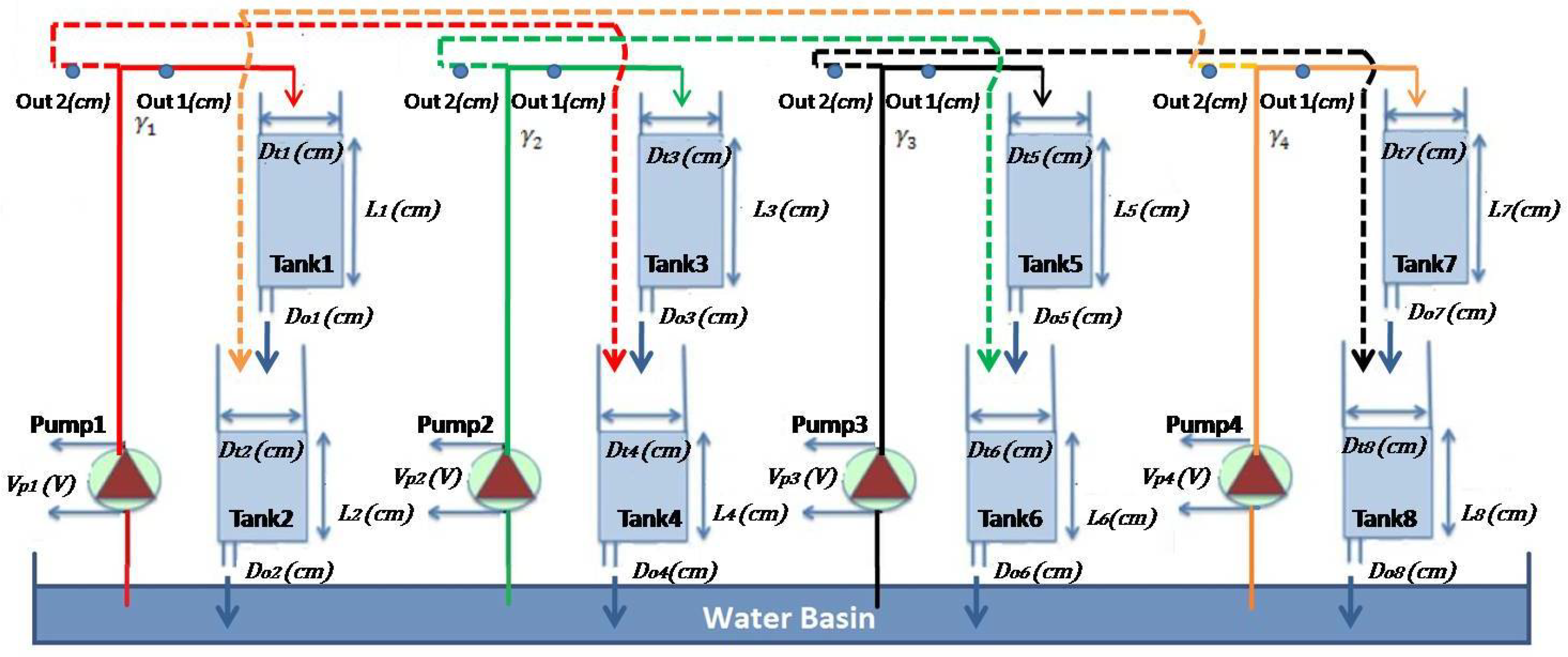
- All three algorithms were tested in simulation on the same process, i.e., the eight-tank process introduced in [40].
- The CC algorithm was based on a matrix gain feedback controller, computed by solving a gradient-based optimization problem. The basic principle of computing the gains was firstly presented in [41].
- The eight-tank process model introduced in [40] was extended with the nonlinear mathematical description based on Bernoulli’s law and the mass balances.
- The DMPC strategies given in [40] are presented in an extended version.
- The gradient-based methodology for computing the gain feedback matrix in the coalitional control framework provided in [41] was reformulated to achieve comparative results with respect to the DMPC strategies. To this end, the feedback gain matrices used in the coalitional control methodology were computed solving a cost function, which minimizes the error between the coalitional state trajectories, with respect to a set of DMPC state trajectories. Moreover, a closed-loop stability constraint was also introduced.
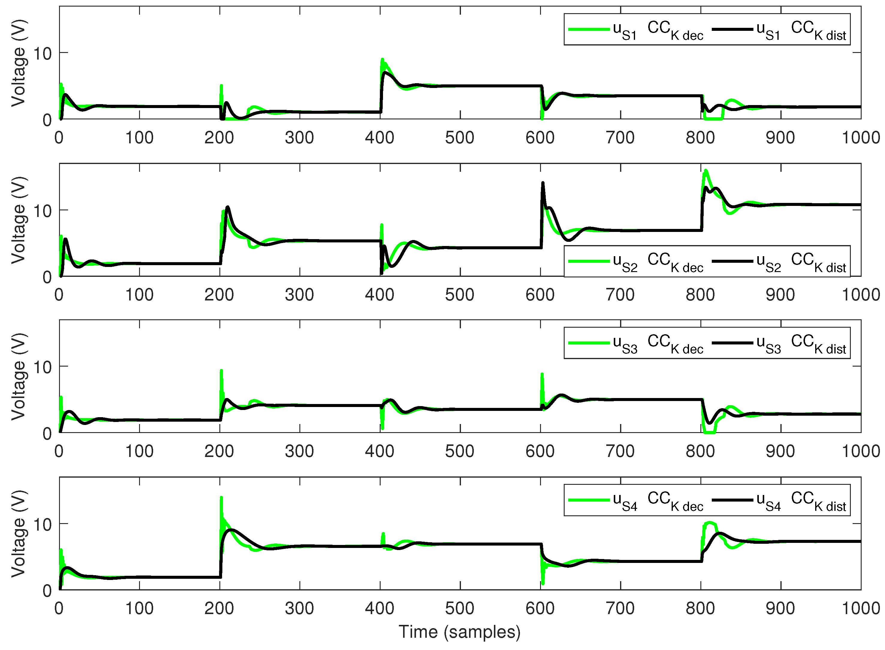
- Two communication topologies were designed for the CC algorithm (with different sets of feedback matrices optimally computed), i.e., a default decentralized communication topology without communication between sub-systems, and a distributed topology with communication links between sub-systems.
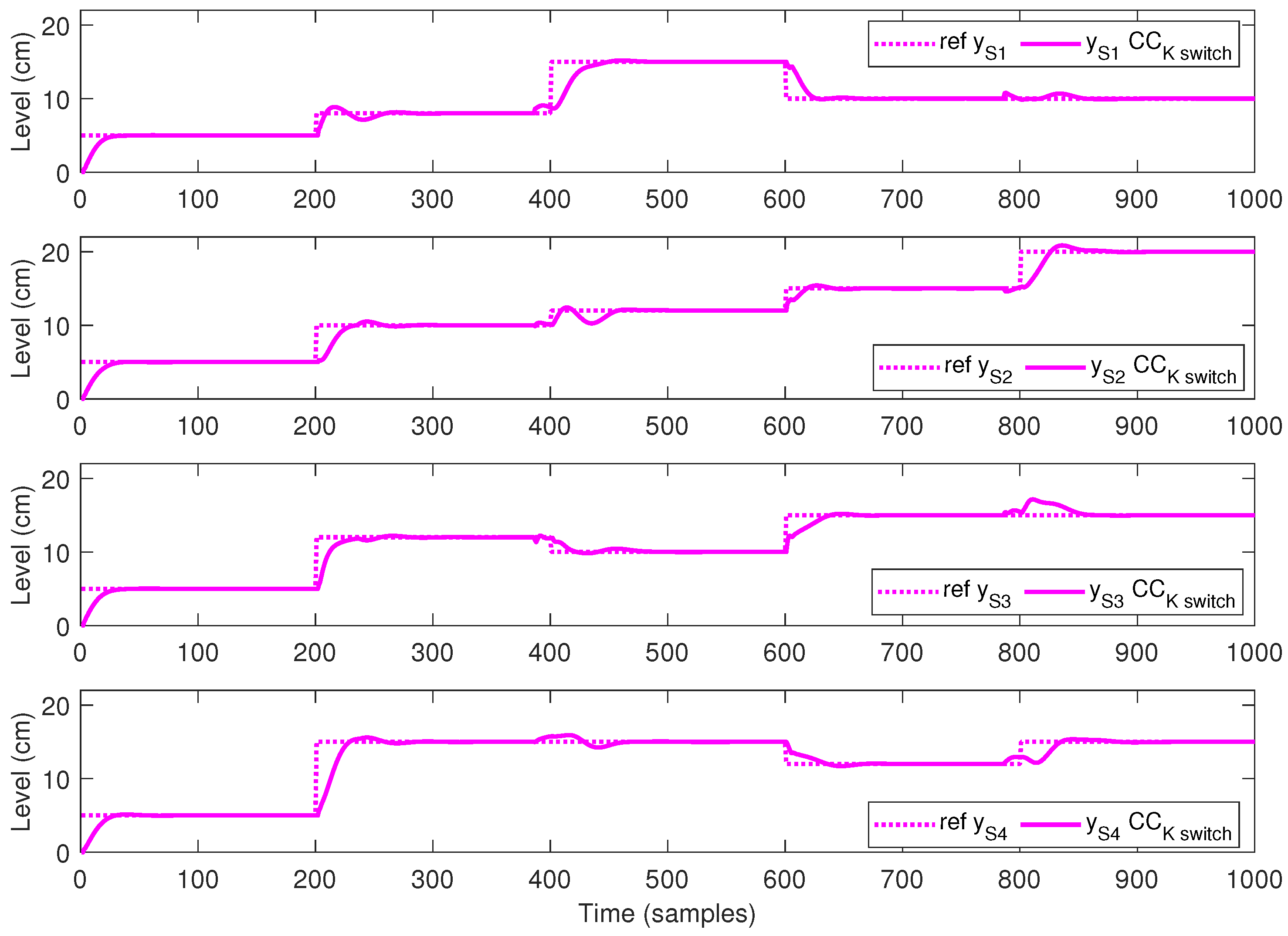
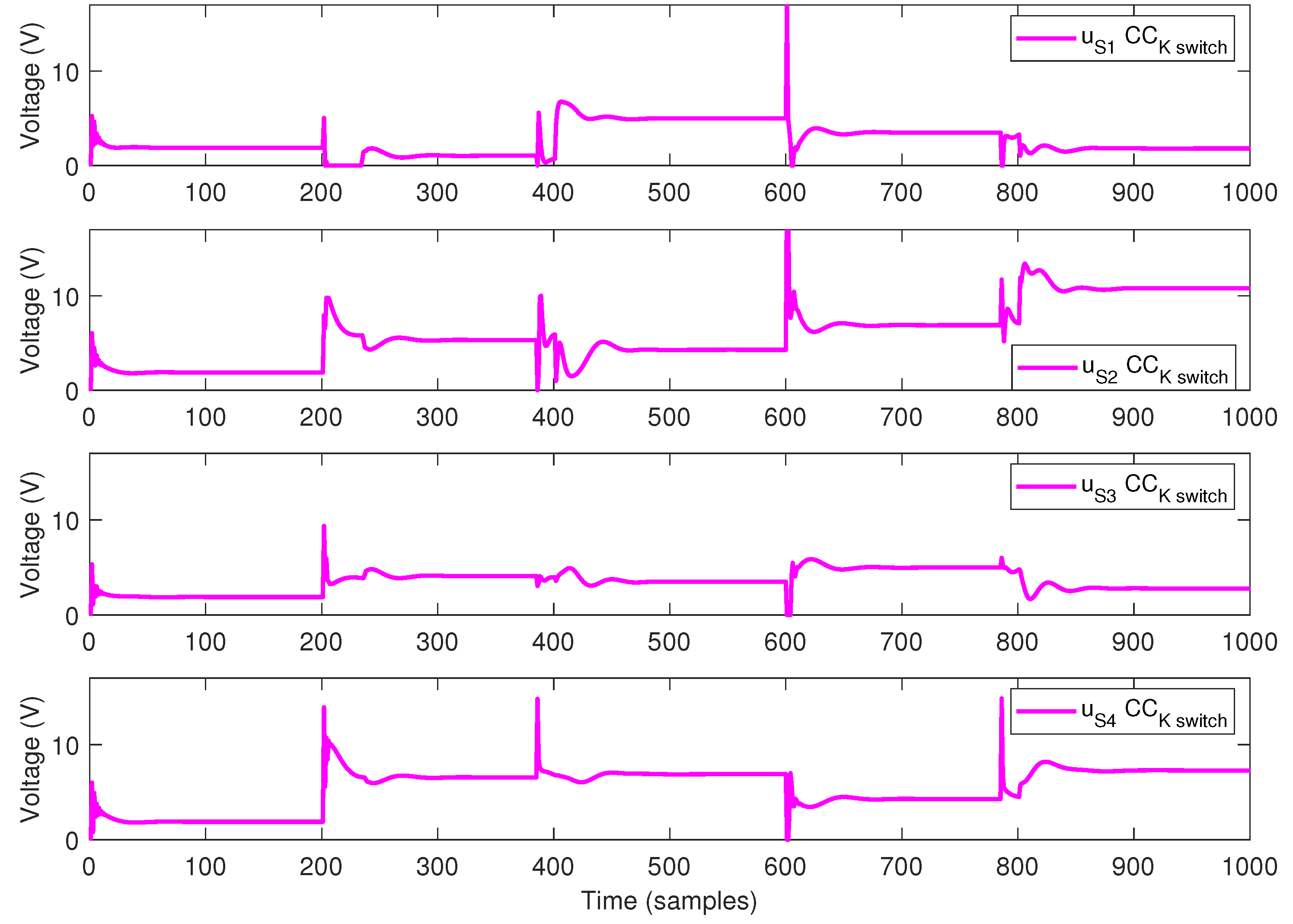
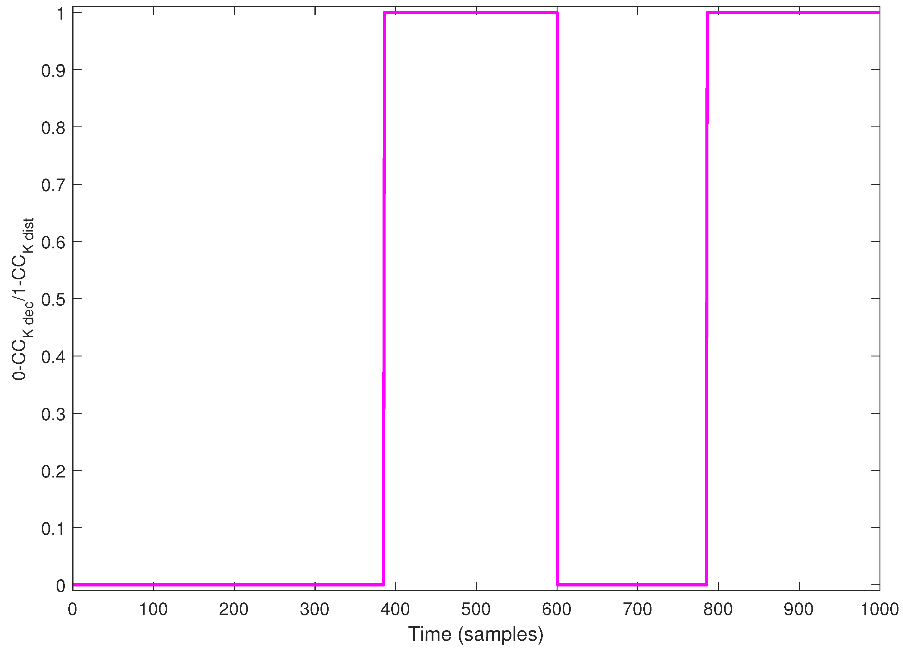
- A procedure that automatically switches between the distributed and decentralized communication topologies designed for the coalitional control methodology is introduced.
2. DMPC Algorithm with State-Space Model (DMPCSS)
2.1. Problem Formulation
2.2. Optimization Problem
3. DMPC Algorithm with Input–Output Model ()
3.1. Problem Formulation
3.2. Optimization Problem
4. Coalitional Control with Gain Feedback Control (CC)
4.1. Problem Formulation
4.2. Optimization Problem
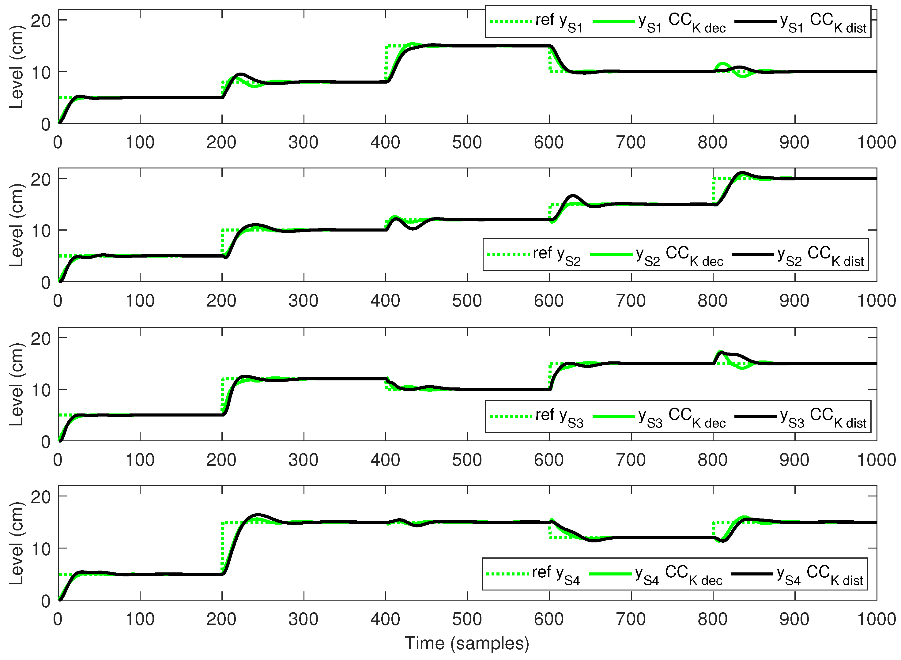
- A decentralized topology, where the control action of the sub-systems is computed without external information; thus, all the communication links are disabled;
- A distributed topology, where the control action of the sub-systems is computed using relevant external information from the neighbours. This means that the communication links between neighbours are enabled.
5. Numerical Analysis on an Eight-Tank Process
5.1. Process Description
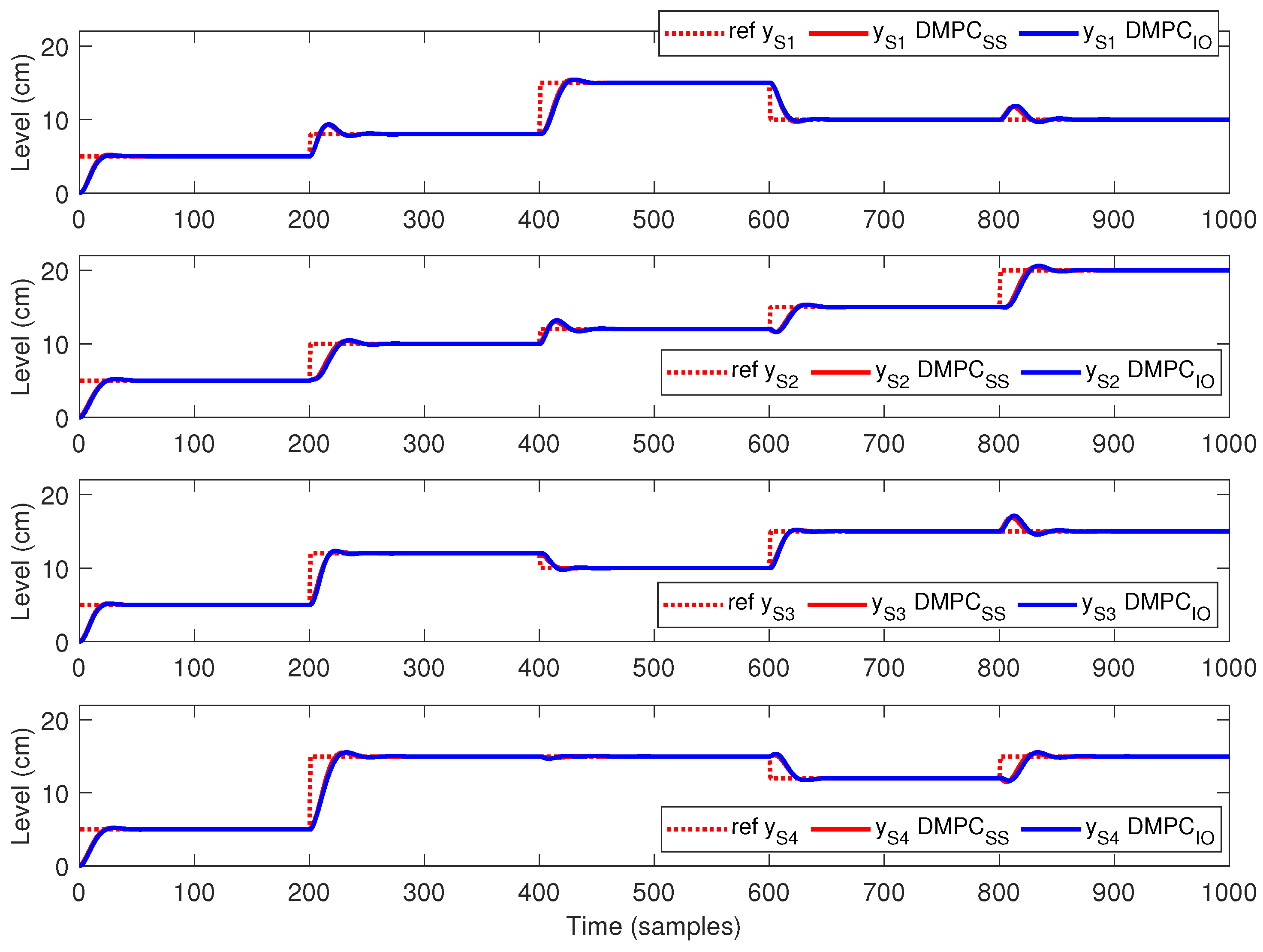
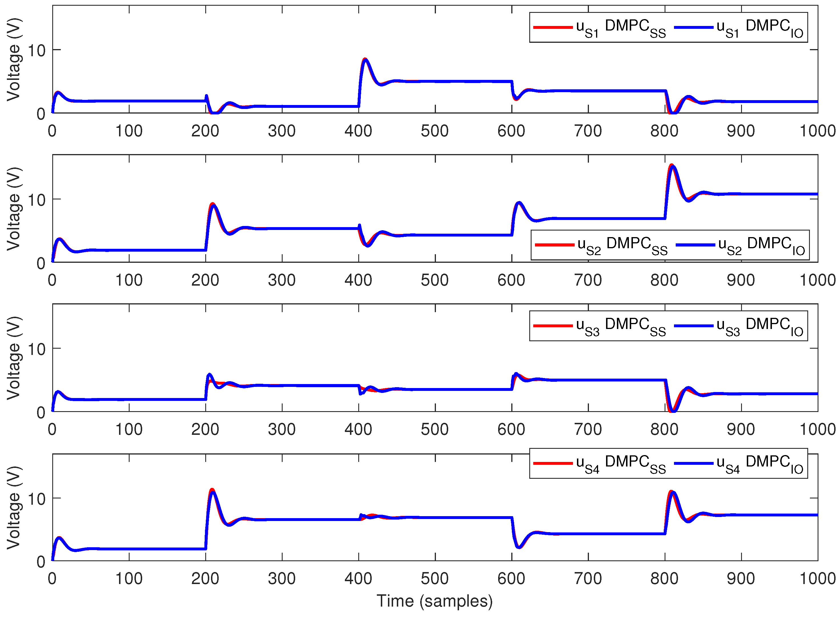
5.2. Simulation Results
- The sampling period 1 s, the prediction horizon = 30 samples and the control horizon = 30 samples;
- The input weight matrices , with , .
- The input weight , the communication cost and the horizon samples.
- The input constraints are , ;
- The output constraints are , .
- During the first 200 s, all references for all sub-systems , are equal to 5 cm.
- At time 201 s, the references values are: cm, cm, cm and cm.
- At time 401 s, the references values are: cm, cm, cm and cm.
- At time 601 s, the references values are: cm, cm, cm and cm.
- At time 801 s, the references values are: cm, cm, cm and cm.
5.3. Discussion
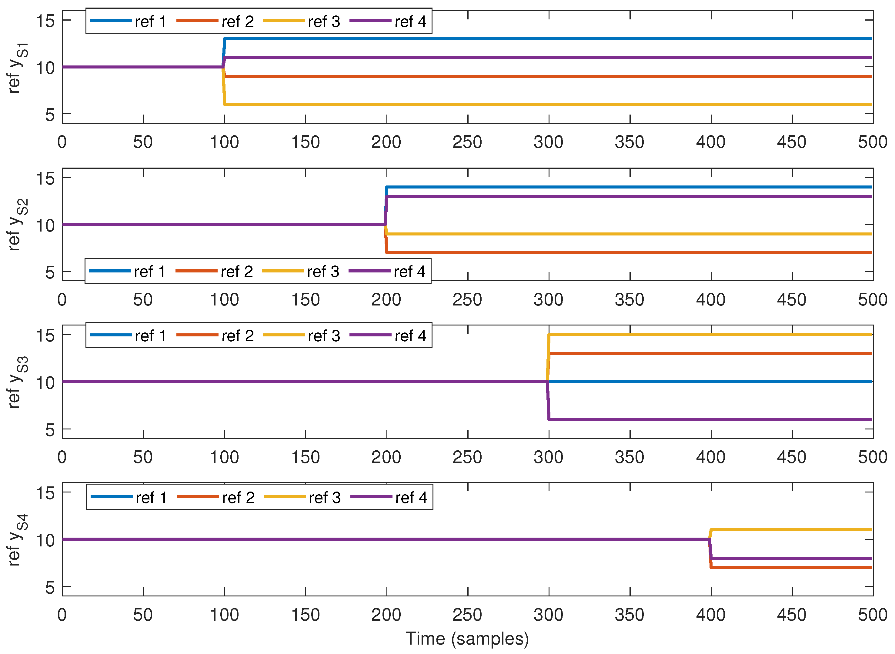
- Length of the simulation time .
- The input weight .
- During the first 100 s, reference cm, at time 101 s, has a step change to a randomly generated value between 5 and 15 cm.
- During the first 200 s, reference cm, at time 201 s, has a step change to a randomly generated value between 5 and 15 cm.
- During the first 300 s, reference cm, at time 301 s, has a step change to a randomly generated value between 5 and 15 cm.
- During the first 400 s, reference cm, at time 401 s, has a step change to a randomly generated value between 5 and 15 cm.
6. Conclusions
Author Contributions
Funding
Institutional Review Board Statement
Informed Consent Statement
Data Availability Statement
Conflicts of Interest
Abbreviations
| MPC | Model Predictive Control |
| DMPC | Distributed Model Predictive Control |
| DMPC with state-space model | |
| DMPC with input–output model | |
| CC | Coalitional Control |
| CC with decentralized communication topology | |
| CC with distributed communication topology | |
| CC with switching communication topology |
References
- Maestre, J.M.; Negenborn, R.R. Distributed Model Predictive Control Made Easy; Springer Science+Business Media: Dordrecht, The Netherlands, 2014. [Google Scholar]
- Espin-Sarzosa, D.; Palma-Behnke, R.; Nuñez-Mata, O. Energy Management Systems for Microgrids: Main Existing Trends in Centralized Control Architectures. Energies 2020, 13, 547. [Google Scholar] [CrossRef]
- Sun, X.; Yin, Y. Decentralized game-theoretical approaches for behaviorally-stable and efficient vehicle platooning. Transp. Res. Part B -Methodol. 2021, 153, 45–69. [Google Scholar] [CrossRef]
- Camacho, E.F.; Bordons, C. Model Predictive Control; Springer: Berlin, Germany, 1999. [Google Scholar]
- Lou, G.; Gu, W.; Xu, Y.; Cheng, M.; Liu, W. Distributed MPC-based secondary voltage control scheme for autonomous drop-control microgrids. IEEE Trans. Sustain. Energy 2017, 8, 792–804. [Google Scholar] [CrossRef]
- Cortés, A.; Martínez, S. On distributed reactive power and storage control on microgrids. Int. J. Robust Nonlinear Control 2016, 16, 3150–3169. [Google Scholar] [CrossRef]
- Liu, M.; Shi, Y.; Liu, X. Distributed MPC of aggregated heterogeneous thermostatically controlled loads in smart grids. Int. Trans. Ind. Electron. 2016, 63, 1120–1129. [Google Scholar] [CrossRef]
- del Real, A.J.; Arce, A.; Bordons, C. Combined environmental and economic dispatch of smart grids using distributed model predictive control. Electr. Power Energy Syst. 2014, 54, 65–76. [Google Scholar] [CrossRef]
- Pham, V.; Ahn, H. Distributed Stochastic MPC Traffic Signal Control for Urban Networks. IEEE Trans. Intell. Transp. Syst. 2023; early access. [Google Scholar] [CrossRef]
- Liu, P.; Ozguner, U.; Zhang, Y. Distributed MPC for cooperative highway driving and energy-economy validation via microscopic simulations. Transp. Res. Part C Emerg. Technol. 2017, 77, 80–95. [Google Scholar] [CrossRef]
- Yan, X.; Cai, B.; Ning, B.; ShangGuan, W. Online distributed cooperative model predictive control of energy-saving trajectory planning for multiple high speed train movements. Transp. Res. Part C Emerg. Technol. 2016, 69, 60–78. [Google Scholar] [CrossRef]
- Kersbergen, B.; van den Boom, T.; de Schutter, B. Distributed model predictive control for railway traffic management. Transp. Res. Part C Emerg. Technol. 2016, 68, 462–489. [Google Scholar] [CrossRef]
- Ferarra, A.; Nai Oleari, A.; Sacone, S.; Siri, S. Freeway as system of systems: A distributed model predictive control scheme. IEEE Syst. J. 2015, 9, 462–489. [Google Scholar] [CrossRef]
- Ye, B.L.; Wu, W.; Mao, W. Distributed model predictive control method for optimal coordination of signal splits in urban traffic networks. Asian J. Control 2015, 17, 775–790. [Google Scholar] [CrossRef]
- Li, H.; Zhang, T.; Zheng, S.; Sun, C. Distributed MPC for Multi-Vehicle Cooperative Control Considering the Surrounding Vehicle Personality. IEEE Trans. Intell. Transp. Syst. 2023; early access. [Google Scholar] [CrossRef]
- Pauca, O.; Maxim, A.; Caruntu, C.F. DMPC-based Data-packet Dropout Compensation in Vehicle Platooning Applications using V2V Communications. In Proceedings of the 2021 European Control Conference, Rotterdam, The Netherlands, 29 June–2 July 2021; pp. 2639–2644. [Google Scholar]
- Maxim, A.; Lazar, C.; Caruntu, C.F. Distributed Model Predictive Control Algorithm with Communication Delays for a Cooperative Adaptive Cruise Control Vehicle Platoon. In Proceedings of the 28th Mediterranean Conference on Control and Automation, Saint-Raphaël, France, 15–18 September 2020; pp. 909–914. [Google Scholar]
- Caruntu, C.F.; Braescu, C.; Maxim, A.; Rafaila, R.C.; Tiganasu, A. Distributed model predictive control for vehicle platooning: A brief survey. In Proceedings of the 20th International Conference on System Theory, Control and Computing, Sinaia, Romania, 13–15 October 2016; pp. 644–650. [Google Scholar]
- Liu, X.; Zhang, Y.; Lee, K.Y. Coordinated distributed MPC for load frequency control of power system with wind farms. IEEE Trans. Ind. Electron. 2017, 64, 5140–5150. [Google Scholar] [CrossRef]
- Spudić, V.; Conte, C.; Baotić, M.; Morari, M. Cooperative distributed model predictive control for wind farms. Optim. Control Appl. Methods 2015, 36, 333–352. [Google Scholar] [CrossRef]
- Zhao, H.; Wu, Q.; Guo, Q.; Sun, H.; Xue, Y. Distributed model predictive control of a wind farm for optimal active power control: Part II: Implementation with clustering based piece-wise affine wind turbine model. IEEE Trans. Sustain. Energy 2015, 6, 840–849. [Google Scholar] [CrossRef]
- Zhang, A.; Yin, X.; Liu, S.; Zeng, J.; Liu, J. Distributed economic model predictive control of wastewater treatment plants. Chem. Eng. Res. Des. 2019, 141, 144–155. [Google Scholar] [CrossRef]
- Foscoliano, C.; Del Vigo, S.; Mulas, M.; Tronci, S. Improving the wastewater treatment plant performance through model predictive control strategies. In Proceedings of the 26th European Symposium on Computer Aided Process Engineering, Portoroz, Slovenia, 12–15 June 2016; pp. 1863–1868. [Google Scholar]
- Albalawi, F.; Durand, H.; Christofides, P.D. Distributed Economic Model Predictive Control with Safeness-Index Based Constraints of a Nonlinear Chemical Process. In Proceedings of the 2018 Annual American Control Conference, Milwaukee, WI, USA, 27–29 June 2018; pp. 2078–2083. [Google Scholar]
- Zhang, S.; Zhao, D.; Spurgeon, S.K.; Yan, X. Distributed Model Predictive Control for the Atmospheric and Vacuum Distillation Towers in a Petroleum Refining Process. In Proceedings of the 11th UKACC International Conference on Control, Belfast, North Ireland, 31 August–2 September 2016. [Google Scholar]
- Ocampo-Martinez, C.; Puig, V.; Cembrano, G.; Quevedo, J. Application of predictive control strategies to the management of complex networks in the urban water cycle. IEEE Control Syst. 2013, 33, 15–41. [Google Scholar]
- Zhao, Z.; Guo, J.; Luo, X.; Lai, C.S.; Yang, P.; Lai, L.; Li, P.; Guerrero, J.; Shahidehpour, M. Distributed Robust Model Predictive Control-Based Energy Management Strategy for Islanded Multi-Microgrids Considering Uncertainty. IEEE Trans. Smart Grid 2022, 13, 2107–2120. [Google Scholar] [CrossRef]
- Shi, Y.; Tuan, H.D.; Savkin, A.V.; Lin, C.T.; Zhu, J.G.; Poor, H.V. Distributed model predictive control for joint coordination of demand response and optimal power flow with renewables in smart grid. Appl. Energy 2021, 209, 116701. [Google Scholar] [CrossRef]
- Liu, Y.; Liu, R.; Wei, C.; Xun, J.; Tang, T. Distributed Model Predictive Control Strategy for Constrained High-Speed Virtually Coupled Train Set. IEEE Trans. Veh. Technol. 2022, 71, 171–183. [Google Scholar] [CrossRef]
- Zhou, Y.; Wang, M.; Ahn, S. Distributed model predictive control approach for cooperative car-following with guaranteed local and string stability. Transp. Res. Part B 2019, 128, 69–86. [Google Scholar] [CrossRef]
- Kong, X.; Ma, L.; Wang, C.; Guo, S.; Abdelbaky, M.A.; Liu, X.; Lee, K.Y. Large-scale wind farm control using distributed economic model predictive scheme. Renew. Energy 2022, 181, 581–591. [Google Scholar] [CrossRef]
- Teng, Y.; Bai, J.; Wu, F.; Zou, H. Explicit distributed model predictive control design for chemical processes under constraints and uncertainty. Can. J. Chem. Eng. 2023; early access. [Google Scholar] [CrossRef]
- Zhang, L.; Wang, J.; Liu, Z.; Li, K. Distributed MPC for tracking based on reference trajectories. In Proceedings of the 33rd Chinese Control Conference, Nanjing, China, 28–30 July 2014; pp. 7778–7783. [Google Scholar]
- Arauz, T.; Chanfreut, P.; Maestre, J.M. Cyber-security in networked and distributed model predictive control. Annu. Rev. Control 2022, 53, 338–355. [Google Scholar] [CrossRef]
- Christofides, P.D.; Scattolini, R.; Muñoz de la Peña, D.; Liu, J. Distributed model predictive control: A tutorial review and future research directions. Comput. Chem. Eng. 2013, 51, 21–41. [Google Scholar] [CrossRef]
- Scattolini, R. Architectures for distributed and hierarchical Model Predictive Control—A review. J. Process Control 2009, 19, 723–731. [Google Scholar] [CrossRef]
- Fele, F.; Maestre, J.M.; Camacho, E.F. Coalitional control: Cooperative game theory and control. IEEE Control Syst. 2017, 37, 53–69. [Google Scholar]
- Chanfreut, P.; Maestre, J.M.; Camacho, E.F. A survey on clustering methods for distributed and networked control systems. Annu. Rev. Control 2021, 52, 75–90. [Google Scholar] [CrossRef]
- Maxim, A.; Caruntu, C.F. A Coalitional Distributed Model Predictive Control Perspective for a Cyber-Physical Multi-Agent Application. Sensors 2021, 21, 4041. [Google Scholar] [CrossRef]
- Maxim, A.; Caruntu, C.F.; Lazar, C.; De Keyser, R.; Ionescu, C.M. Comparative Analysis of Distributed Model Predictive Control Strategies. In Proceedings of the 23rd International Conference on System Theory, Control and Computing, Sinaia, Romania, 9–11 October 2019; pp. 468–473. [Google Scholar]
- Maxim, A.; Pauca, O.; Maestre, J.M.; Caruntu, C.F. Assessment of computation methods for coalitional feedback controllers. In Proceedings of the 2022 European Control Conference, London, UK, 12–15 July 2022; pp. 1448–1453. [Google Scholar]
- Maxim, A.; Ionescu, C.M.; Caruntu, C.F.; Lazar, C.; De Keyser, R. Reference Tracking using a Non-Cooperative Distributed Model Predictive Control Algorithm. In Proceedings of the 11th IFAC Symposium on Dynamics and Control of Process Systems, including Biosystems, Trondheim, Norway, 6–8 June 2016; pp. 1079–1084. [Google Scholar]
- Maxim, A.; Copot, D.; De Keyser, R.; Ionescu, C.M. An industrially relevant formulation of a distributed model predictive control algorithm based on minimal process information. J. Process Control 2018, 68, 240–253. [Google Scholar] [CrossRef]
- De Keyser, R.; Ionescu, C.M. The disturbance model in model based predictive control. In Proceedings of the 2003 IEEE Conference on Control Applications, Istanbul, Turkey, 25–25 June 2003; pp. 446–451. [Google Scholar]
- De Keyser, R. Model Based Predictive Control for Linear Systems. In UNESCO Encyclopaedia of Life Support Systems, Control Systems, Robotics and Automation—Vol. XI, Article Contribution 6.43.16.1; Eolss Publishers Co. Ltd.: Oxford, UK, 2003; Available online: http://www.eolss.net/sample-chapters/c18/e6-43-16-01.pdf (accessed on 1 January 2023).
- Maxim, A.; Ionescu, C.M.; Copot, C.; De Keyser, R.; Lazar, C. Multivariable model-based control strategies for level control in a quadruple tank process. In Proceedings of the 17th International Conference on System Theory, Sinaia, Romania, 11–13 October 2013; pp. 343–348. [Google Scholar]


| Variable | Value | Unit | Description |
|---|---|---|---|
| 0.635 | cm | “Out 1” Orifice diameter | |
| 0.476 | cm | “Out 2” Orifice diameter | |
| 4.445 | cm | Inner diameter Tank i, | |
| 0.476 | cm | Outlet diameter Tank i, | |
| 0.6402 | - | Flow ratio parameter for Pump i, | |
| 0.316 | Inlet area Tank i, | ||
| 0.178 | Inlet area Tank i, | ||
| 15.517 | Inside cross-section area Tank i, | ||
| 0.178 | Outlet area Tank i, | ||
| 3.3 | Pump flow constant | ||
| g | 981 | Gravitational constant on Earth |
| Algorithm | (%) | tt (s) | |
|---|---|---|---|
| 4.6103 | 3.9102 | 33 | |
| 5.0120 | 2.3250 | 31 | |
| 4.4757 | 0 | 29 | |
| 5.4070 | 4.6806 | 54 | |
| 4.4682 | 0 | 30 |
| Algorithm | ||||||||||
|---|---|---|---|---|---|---|---|---|---|---|
| 7.06 | 6.9232 | 7.234 | 6.9941 | 7.4663 | 7.1101 | 6.2858 | 7.5058 | 7.1761 | 7.2923 | |
| 3.8399 | 3.7616 | 3.9228 | 3.7897 | 4.0333 | 3.8603 | 3.4247 | 4.5454 | 3.9086 | 3.9745 | |
| 6.6852 | 6.5503 | 6.9014 | 6.6434 | 7.1358 | 6.7618 | 5.8971 | 7.1275 | 6.7765 | 6.957 | |
| 8.0269 | 7.9341 | 8.3214 | 7.9283 | 8.6276 | 8.1404 | 7.1244 | 8.4239 | 8.1521 | 8.3999 | |
| 6.6852 | 6.6496 | 6.9014 | 6.6434 | 7.2027 | 6.708 | 5.8971 | 7.1338 | 6.9815 | 7.0748 | |
| Algorithm | ||||||||||
| 7.1924 | 7.8314 | 7.9128 | 6.8795 | 7.1698 | 7.5848 | 7.3844 | 6.8498 | 6.684 | 7.3929 | |
| 3.906 | 4.6893 | 4.278 | 3.7476 | 3.8727 | 4.1029 | 4.0108 | 3.7335 | 3.6424 | 4.0175 | |
| 6.8137 | 7.4959 | 7.5955 | 6.529 | 6.8305 | 7.2667 | 7.0623 | 6.4549 | 6.3308 | 7.0272 | |
| 8.1562 | 10.0325 | 9.0328 | 7.8895 | 8.2037 | 8.7419 | 8.5967 | 7.7314 | 7.6851 | 8.5349 | |
| 6.8137 | 7.3403 | 7.5955 | 6.7604 | 6.8305 | 7.3402 | 7.0623 | 6.4549 | 6.3626 | 7.0342 | |
| Algorithm | ||||||||||
| 6.6234 | 6.526 | 7.534 | 8.3664 | 8.869 | 6.8697 | 6.9339 | 7.4802 | 6.8035 | 6.4023 | |
| 3.6011 | 3.5644 | 4.2458 | 4.5478 | 6.5396 | 3.7348 | 3.7476 | 4.0698 | 3.7181 | 3.4967 | |
| 6.2535 | 6.1489 | 7.1624 | 8.0334 | 8.5175 | 6.5079 | 6.588 | 7.1204 | 6.4382 | 6.016 | |
| 7.4819 | 7.4183 | 8.8481 | 9.691 | 10.2905 | 7.8125 | 7.9544 | 8.5508 | 7.7259 | 7.2463 | |
| 6.2535 | 6.1489 | 7.4142 | 8.434 | 8.5175 | 6.5079 | 6.588 | 7.1204 | 6.4382 | 6.016 | |
| Algorithm | ||||||||||
| 10.0696 | 7.6568 | 6.1639 | 6.9149 | 7.0216 | 6.7982 | 8.2884 | 7.6686 | 8.1218 | 6.5389 | |
| 7.3631 | 4.1428 | 3.3615 | 3.7589 | 3.8114 | 3.708 | 5.2155 | 4.1158 | 4.3801 | 3.5525 | |
| 9.7118 | 7.2916 | 5.7669 | 6.5551 | 6.6673 | 6.4463 | 7.9295 | 7.3523 | 7.8033 | 6.1602 | |
| 11.4071 | 8.7722 | 6.9522 | 7.8125 | 8.0195 | 7.795 | 9.2517 | 8.8459 | 9.3484 | 7.4062 | |
| 9.9748 | 7.2916 | 5.7669 | 6.6249 | 6.7133 | 6.4463 | 7.9884 | 7.6813 | 7.8033 | 6.2888 | |
| Algorithm | ||||||||||
| 7.9808 | 7.4112 | 7.6753 | 7.3881 | 8.3035 | 6.7645 | 7.0579 | 7.3141 | 7.4849 | 7.1852 | |
| 4.2934 | 4.347 | 4.1347 | 4.0217 | 4.5533 | 3.6815 | 3.8437 | 3.9524 | 4.035 | 3.8977 | |
| 7.6536 | 7.0194 | 7.3547 | 7.0098 | 7.9717 | 6.4051 | 6.6749 | 6.9475 | 7.1379 | 6.7994 | |
| 9.0457 | 8.8949 | 8.8047 | 8.3742 | 9.8268 | 7.7782 | 7.9759 | 8.2984 | 8.4842 | 8.1058 | |
| 7.494 | 7.7026 | 7.3214 | 7.0098 | 7.8147 | 6.5034 | 6.6749 | 7.1071 | 7.2662 | 6.7994 |
Disclaimer/Publisher’s Note: The statements, opinions and data contained in all publications are solely those of the individual author(s) and contributor(s) and not of MDPI and/or the editor(s). MDPI and/or the editor(s) disclaim responsibility for any injury to people or property resulting from any ideas, methods, instructions or products referred to in the content. |
© 2023 by the authors. Licensee MDPI, Basel, Switzerland. This article is an open access article distributed under the terms and conditions of the Creative Commons Attribution (CC BY) license (https://creativecommons.org/licenses/by/4.0/).
Share and Cite
Maxim, A.; Pauca, O.; Caruntu, C.-F. Distributed Model Predictive Control and Coalitional Control Strategies—Comparative Performance Analysis Using an Eight-Tank Process Case Study. Actuators 2023, 12, 281. https://doi.org/10.3390/act12070281
Maxim A, Pauca O, Caruntu C-F. Distributed Model Predictive Control and Coalitional Control Strategies—Comparative Performance Analysis Using an Eight-Tank Process Case Study. Actuators. 2023; 12(7):281. https://doi.org/10.3390/act12070281
Chicago/Turabian StyleMaxim, Anca, Ovidiu Pauca, and Constantin-Florin Caruntu. 2023. "Distributed Model Predictive Control and Coalitional Control Strategies—Comparative Performance Analysis Using an Eight-Tank Process Case Study" Actuators 12, no. 7: 281. https://doi.org/10.3390/act12070281
APA StyleMaxim, A., Pauca, O., & Caruntu, C.-F. (2023). Distributed Model Predictive Control and Coalitional Control Strategies—Comparative Performance Analysis Using an Eight-Tank Process Case Study. Actuators, 12(7), 281. https://doi.org/10.3390/act12070281