Determination of the Optimal Order of Grey-Box Models for Short-Time Prediction of Buildings’ Thermal Behavior

Abstract

The use of grey-box models for short-time forecasting of buildings’ thermal behavior requires the determination of the models’ order since this order could influence the grey-box models’ performance. This paper presents an analysis of the optimal order of these models for different thermal conditions. The novelty of this work consists of considering the influence of the heating conditions on the determination of the performances of grey-box models. The analysis is based on experimental tests that were conducted in a room with different thermal conditions, related to the variation of the heating power. Experimental results were used for the determination of the optimal grey-box models’ order that minimizes the gap between the experimental results and the grey-box forecasting. Results show that the optimal grey-box models’ order depends on the buildings’ thermal conditions, but generally lies between two and three with an error less than 0.2 °C and a fit percent greater than 90%.

1. Introduction

Building energy simulation models (white models) require a good understanding of the thermal behavior of buildings [1]. Since the use of these models requires detailed information about the buildings’ components, equipment and use, as well as large computation capacities [2,3], alternative thermal models were proposed for the thermal modelling of buildings such as the black-box models [4,5] and grey-box models [6,7].

The grey-box models provide some advantages in the buildings’ thermal modeling process, in particular, ease of their use and the possibility to link their parameters to global buildings’ physical characteristics, such as the heat resistance and the mass capacity. These models can be used for different purposes such as control of the indoor environment [8,9], forecasting energy consumption, and evaluating buildings’ energy performance [10,11,12]. However, their practical use is subjected to the difficulty of the determination of their optimal order. This issue was investigated recently in some papers [6,13]. For unoccupied buildings, Bacher and Madson [14] showed that the performances of the grey-box were not improved by increasing the model order beyond 3. Hedgaard and Peterson [13] showed that the second and third-order models produce a good short-time forecasting of the building’s thermal behavior. Fonti et al. [15] used experimental studies to analyze the accuracy of grey-box models for the short-term prediction of a building. Results showed that the second-order models provide the required accuracy. Reynders et al. [16] carried out an identification study to determine suitable reduced-order models for predicting the thermal response of a residential building. They found out that best predictions were obtained with the third-order grey-box model.

Generally, the grey-box models’ order is presumed independent of the power supply conditions. In recent research [17], it was shown that the heating conditions should be considered in the determination of the optimal order of the grey-box models and that the data dynamics affect the performance of grey-box models. This paper discusses this issue using experimental tests conducted in various heating conditions for the investigation of the influence of these conditions on the optimal order of the grey-box model.

2. Methodology

Tests were carried out in a room submitted to various thermal conditions. The indoor temperature, as well as the external temperature, were recorded. Tests were conducted with three values of the indoor heating power (zero, 900 W and 1500 W). The results of each test were then used for the analysis of the grey-box models’ performances for three forecasting times: 15, 30, and 60 min. Analyses were conducted with four values of the grey-box order: 1, 2, 3 and 4 (Figure 1). The optimal order of the grey-box model for each experiment was then determined by comparing the numerical simulations to recorded data.

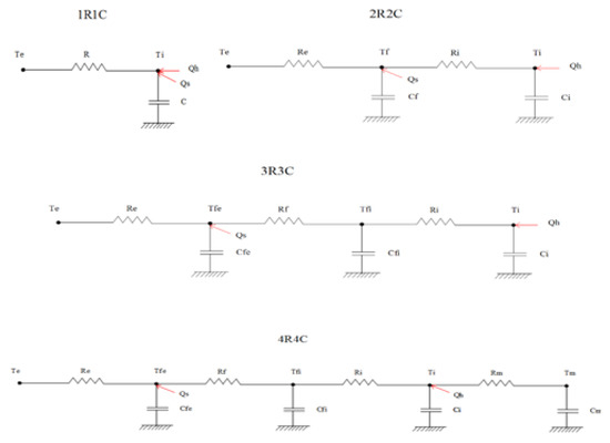
Figure 1. Resistor-Capacitor networks for the four models.

Numerical simulations were performed using MATLAB software.

2.1. Grey Box Modeling

Grey box models combine building physics and statistics. Physical knowledge derived from the buildings’ dynamics is formulated by stochastic differential equations in the state space form [15]. Statistical measurements present information embedded in the collected data.

$$\mathrm{dX}\left(\mathrm{t}\right)=\mathrm{A}\left(\mathsf{\theta }\right)\mathrm{X}\left(\mathrm{t}\right)+\mathrm{B}\left(\mathsf{\theta }\right)\mathrm{U}\left(\mathrm{t}\right)+\mathsf{\sigma }\left(\mathsf{\theta }\right)\mathrm{dw},\mathrm{Y}\left(\mathrm{t}\right)=\mathrm{C}\left(\mathsf{\theta }\right)\mathrm{X}\left(\mathrm{t}\right)+\mathrm{D}\left(\mathsf{\theta }\right)\mathrm{U}\left(\mathrm{t}\right)+\mathsf{\epsilon }$$

(1)

Sun radiation is considered zero due to the absence of windows. Parameters θ were estimated using MATLAB software. The model structures are derived from (RC) networks, analogue to the electric circuit.

The parameters of the model represent different thermal properties of the building. This includes thermal resistances: R, R_e, R_i, R_m, and R_f.

The heat capacities of different parts of the building are represented by: C, C_i, C_fe and C_fi and C_m.

Finally, the input vector consists of T_e and the internal energy sources which are presented by Q_s and Q_h.

An example of a simple model (1R1C) is given here. By applying the dynamic heating balance equation, we get:

$$\mathrm{C}\frac{\mathrm{dTi}}{\mathrm{dt}}=\frac{1}{\mathrm{R}}\left(\mathrm{Te}-\mathrm{Ti}\right)+\mathrm{heating}\mathrm{source},\mathrm{C}\frac{\mathrm{dTi}}{\mathrm{dt}}=\frac{1}{\mathrm{R}}\left(\mathrm{Te}-\mathrm{Ti}\right)+\mathrm{Qs}+\mathrm{Qh}$$

(2)

Same methodology was applied for the other orders.

2.2. Parameters Estimation

The model’s parameters were determined using ‘Greyest’ function in ‘Matlab’. This function provides the maximum likelihood using the following algorithms: The Gauss-Newton direction, the Levenberg-Marquardt and the steepest descent gradient [15,18].

Initialization of parameters was calculated by applying the French thermal code (RT 2005–2012), see Appendix A [11,19,20]. Table 1 presents the initial values of the parameters defining buildings’ characteristics.

Table 1. Initial values for the estimated parameters.

Estimated Parameter	Value
Ci (J/K)	1.47 × 105
Cfe (J/K)	1.77 × 108
Cfi (J/K)	9.36 × 106
Cm (J/K)	4.54 × 106
Ri, Rm (K/W)	1.82 × 10−2
Re (K/W)	3 × 10−3
Rf (K/W)	1.1 × 10−1

The performance of the model is evaluated by (i) the root-mean-square error (RMSE-values); (ii) the final prediction errors (FPE); (iii) the level of fit (FIT) or normalized root mean square error (NRMSE) and (iv) the auto-correlation of the residuals [21]. The error distribution ‘e’ between the predicted and recorded temperatures is also determined (e is evaluated by subtracting the predicted value from the recorded one than a distribution analysis was carried out.).

A sensitivity study was performed by calculating the Sobol index to verify that all estimated models’ parameters are necessary for the predictions. This method allows measuring the overall impact of a parameter in the output of the model. When the Sobol index is high (close to 1), the parameter has a strong impact on the model.

Saltelli [22] and Jansen [23] proposed the following expression for the Sobol index:

$${\mathrm{ST}}_{\mathrm{i}}=\frac{\frac{1}{2\mathrm{N}}{{\displaystyle \sum }}_{\mathrm{w}=1}^{\mathrm{N}}({\mathrm{Y}}_{\mathrm{b}}-{\mathrm{Y}}_{\mathrm{ci})}{}^2}{\mathrm{Var}\left({\mathrm{Y}}_{\mathrm{a}},{\mathrm{Y}}_{\mathrm{b}}\right)},$$

(3)

The model comparative criterion (Y) is the Root Mean Squared Error (RMSE, Equation (4)) between the predicted data and the reference data. The quasi-random LHS (Latin hypercube sampling) type method is used to accelerate the convergence. All parameters vary by plus or minus 30% of their adjusted value (values after learning).

$$\mathrm{RMSE}=\sqrt{\frac{{\sum }_{\mathrm{i}=1}^{\mathrm{n}}{\left({\mathrm{y}}_{\mathrm{i}}-{\hat{\mathrm{y}}}_{\mathrm{i}}\right)}^2}{\mathrm{n}}},$$

(4)

For each dataset, the most performing order are investigated. A parameter cannot be identified correctly if its variation does not impact output values. Therefore, it is necessary to have high values of the total Sobol index for all parameters to validate the model architecture.

3. Experimental Data

A smart monitoring system was installed in a room of a research building ‘A4’ at Lille University in the north of France. The room is formed of two façades and two internal walls without windows. The following experiments were conducted (Table 2):

Table 2. Conducted experiments.

Experiment	Indoor Heating Power (W)
A	0
B	900
C	1500

-

Experiment A: The room was submitted only to external thermal condition without any indoor heating power.

-

Experiment B: The room was submitted to the external thermal conditions as well as to an indoor 900 W heating power.

-

Experiment C: The room was submitted to the external thermal conditions as well as to an indoor 1500 W heating power.

Figure 2 shows the variation of the indoor temperature for low and high heating levels. This graph indicates that for 4 hours high heating, 18 minutes (min) has been needed for a variation of 1 °C, while 30 min is needed for low heating. By decreasing the heating time of 2 hours, 12 min are needed for a variation of 1 °C at 1500 W heating. We noticed that for high heating, 25 min are needed to achieve a variation of 1 °C for the difference between the indoor and outdoor temperatures, while 40 min are needed for low heating. By decreasing the heating time of 2 hours, 15 min is needed for a variation of 1 °C at 1500 W heating. Consequently, it is necessary to execute prediction for 15 min, 30 min, and 60 min to cover the phase of façade heating exchange.

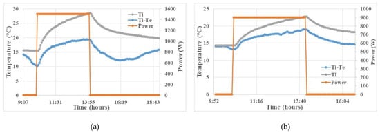
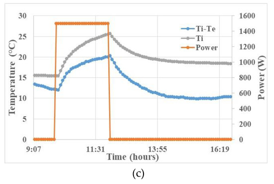
Figure 2. Variation of indoor and outdoor temperature while heating: (a) 4 hours heating at 1500 W; (b) 4 hours heating at 900 W; (c) 2 hours heating at 1500 W.

4. Results and Discussion

For each dataset, the prediction is executed for 15, 30 and 60 min for the first, second, third and fourth order. To simplify the comparison, results will be presented in terms of RMSE and fit percent to determine the best performing models and to evaluate the impact of the dynamics of data on the predictions quality.

4.1. Sensitivity Analysis

Sensitivity analysis was conducted to confirm the significant role of chosen parameters [24]. Table 3 presents the result of this analysis. It shows that all parameters have an important influence on forecasting values. Figure 3 indicates that for tests B and C, the "R_i" parameter is among the two highest indices. This parameter represents the thermal resistance of indoor air in the building. It shows that this phenomenon has a preponderant impact on the thermal behavior of the building.

Table 3. Calculated total Sobol index.

Result	Free-Floating (Test A)		Heating - 900W (Test B)						Heating - 1500W (Test C)
Parameter	C	R	Ci	Cfe	Cfi	Ri	Re	Rf	Ci	Cf	Ri	Re
STi	0.98	0.99	0.07	0.09	0.24	0.60	0.12	0.18	0.62	0.85	0.72	0.59

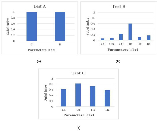
Figure 3. Results of sensibility analysis: (a)Test A; (b) Test B; (c) Test C.

We noticed that for test B, C_i and C_fe have low total Sobol indices comparing to other parameters (0.07 and 0.09), but their values are not negligible. This can be referred to the subjection of these parameters to a small amplitude of variation (± 30%) compared to the dispersion observed in a real building.

This sensitivity analysis showed that the totality of identified parameters had an important role in predicting the building’s thermal behavior.

4.2. Experiment A (Heating Power = 0)

Table 4 illustrates the influence of the order of grey-box model on the quality of temperature predictions at 15 minutes. It could be observed that the optimal order of the grey-box model is equal to 2 (RMSE equal to 0.0616), with a slight difference with orders 1 and 3, which have RMSEs equal to 0.0656 and 0.0648, respectively. Table 5 and Table 6 illustrate the influence of the order of grey-box model on the quality of temperature predictions at 30 and 60 minutes. This influence is similar to that of 15 minutes. Since by increasing the model order above 1, the improvement in the temperature prediction is negligible, order 1 could be retained for this dataset as the simplest structure. Models of fourth order did not converge for all predictions because this experiment does not include any excitation source. Similar results were provided by Reynders et al. [16].

Table 4. Fifteen-minute prediction results for expirment A.

Result	1R1C	2R2C	3R3C	4R4C
Fit percent	95.11	95.35	95.12	10.09
RMSE	0.0656	0.0616	0.0648	1.2004

Table 5. Thirty-minute prediction results for experiment A.

Result	1R1C	2R2C	3R3C	4R4C
Fit percent	91.86	92.91	91.97	-
RMSE	0.1086	0.0949	0.1072	-

Table 6. Sixty-minute prediction results for experiment A.

Result	1R1C	2R2C	3R3C	4R4C
Fit percent	87.83	90.24	88.05	-
RMSE	0.1625	0.1304	0.1594	-

Figure 4 shows the error distribution corresponding to the first order. It could be observed that about 99% of the data have an error of less than 0.5 °C for 15, 30, and 60 min predictions. Model of order one can be used effectively for 1-hour prediction (large-step forecasting), which is considered adequate for heating control.

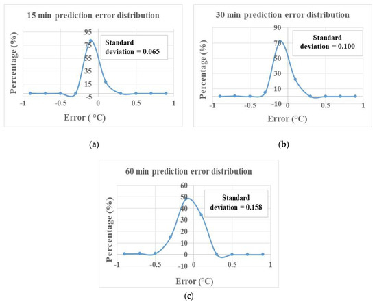
Figure 4. Error distribution for experiment A-order 1: (a) 15 min prediction; (b) 30 min prediction (c) 60 min prediction.

4.3. Experiment B (Heating Power = 900 W)

Table 7, Table 8 and Table 9 illustrate the influence of the grey-box models’ order on the temperature predictions at 15, 30, and 60 minutes. It could be observed that the optimal order is equal to 3, with a slight difference with order 2. Models of first order do not converge for all predictions. This result is similar to the those obtained in [25], because this order is not sufficient to explain the data dynamics.

Table 7. Fifteen-minute prediction results for experiment B.

Result	1R1C	2R2C	3R3C	4R4C
Fit percent	-	93.97	95.43	44.15
RMSE	-	0.1204	0.0917	1.1170

Table 8. Thirty-minute prediction results for experiment B.

Result	1R1C	2R2C	3R3C	4R4C
Fit percent	-	87.6	92.98	36.52
RMSE	-	0.2480	0.1404	1.2697

Table 9. Sixty-minute prediction results for experiment B.

Result	1R1C	2R2C	3R3C	4R4C
Fit percent	-	80.65	90.71	31.25
RMSE	-	0.3869	0.1857	1.3751

Models of fourth order become more sensitive and complex for this set of data.

Figure 5 shows the error distribution corresponding to the third order. It could be observed that about 99% of the data have an error of less than 0.5 °C for 15- and 30-min predictions and 97% for 60-min predictions.

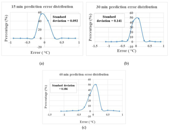
Figure 5. Error distribution for experiment B-order 3: (a) 15 min prediction; (b) 30 min prediction (c) 60 min prediction.

Figure 6 illustrates the residuals’ auto-correlation for order 3 obtained with a lag of 25. The yellow interval shows a 99% limit of confidence, which indicates that this model describes well the building dynamics.

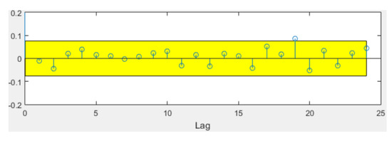
Figure 6. Residual autocorrelation—Experiment B—order 3.

4.4. Experiment C (Heating Power = 1500 W)

Table 10, Table 11 and Table 12 illustrate the influence of the order of the grey-box model on the temperature predictions at 15, 30 and 60 minutes. It could be observed that the optimal order is equal to 2, with a slight difference with orders 3 and 4. Results show that this dataset explains the best the building’s dynamics since all models’ orders present satisfactory performances with the greatest fit percentage and the lowest RMSE. This confirms the results obtained in [15], where the order 2 was the most performing order with RMSE less than 0.5 °C and fit percent equal to 94% for 1-hour prediction.

Table 10. Fifteen-minute prediction results for experiment C.

Result	1R1C	2R2C	3R3C	4R4C
Fit percent	93.36	97.2	95.7	96.18
RMSE	0.2349	0.0990	0.1523	0.1353

Table 11. Thirty-minute prediction results for experiment C.

Result	1R1C	2R2C	3R3C	4R4C
Fit percent	83.34	95.56	90.7	92.17
RMSE	0.5895	0.1572	0.3291	0.2769

Table 12. Sixty-minute prediction results for experiment C.

Result	1R1C	2R2C	3R3C	4R4C
Fit percent	71.49	93.54	84.71	87.59
RMSE	1.0090	0.2285	0.5410	0.4392

Figure 7 shows the error distribution corresponding to the second order. It could be observed that about 99% of the data have an error of less than 0.5 °C for 15- and 30-min predictions and 97% for 60-min predictions.

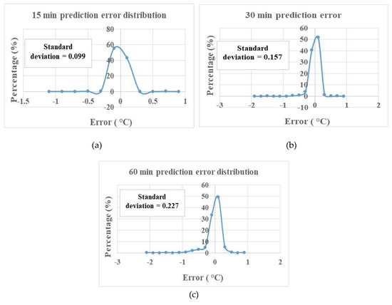
Figure 7. Error distribution for experiment C-order 2: (a) 15 min prediction; (b) 30 min prediction (c) 60 min prediction.

Figure 8 shows the residuals’ auto-correlation for order 2 with a lag of 25. The yellow interval indicates a 99% limit of confidence. This figure indicates that this model describes the building dynamics well.

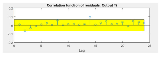
Figure 8. Residual autocorrelation—Experiment C—order 2.

By analyzing the previous results, we noticed that the choice of the model’s order depended on the data dynamics. The prediction for the most reliable order for all the data sets present performing results for short term forecasting. Dynamic data with heating at 1500 W reveal the most buildings’ dynamics. We can notice the need for an automated process combining many datasets and grey-box models able to determine the most performing order for the best dataset revealing the real dynamics of the building.

5. Conclusions

This paper presented a method for the determination of the optimal order of the grey-box models used in forecasting building’s thermal behavior in different thermal conditions. Experiments were conducted in a monitored room with three values of the heating power. These experiments were used for the analysis of the influence of the order of the grey-box models on the quality of the short-time forecasting of the indoor temperature. Results show that the optimal order of the grey-box models depends on the buildings’ thermal conditions, but generally lies between 2 and 3 with an error less than 0.2 °C and a fit percent greater than 90% for all prediction times. Analyses indicate that in the case of dynamic heating, the first order is not sufficient for the identification process. This study reveals a need for data in different heating conditions to determine the optimal order of the grey-box models.

References

- Brastein, O.M.; Perera, D.W.U.; Pfeifer, C.; Skeie, N.O. Parameter estimation for grey-box models for building thermal behavior. Energy Build. 2018, 169, 58–68. [Google Scholar] [CrossRef]
- Crawley, D.B.; Hand, J.W.; Kummert, M.; Griffith, B.T. Contrasting the capabilities of building energy performance simulation programs. Build. Environ. 2008, 43, 661–673. [Google Scholar] [CrossRef]
- Liu, S.; Henze, G.P. Experimental analysis of simulated reinforcement learning control for active and passive building thermal storage inventory. Energy Build. 2006, 38, 142–147. [Google Scholar] [CrossRef]
- Kalogirou, S. Artificial neural networks for the prediction of the energy consumption of a passive solar building. Energy 2000, 25, 479–491. [Google Scholar] [CrossRef]
- Attoue, N.; Shahrour, I.; Younes, R. Smart building: Use of the artificial neural network approach for indoor temperature forecasting. Energies 2018, 11, 395. [Google Scholar] [CrossRef]
- Wang, Z.; Chen, Y.; Li, Y. Development of RC model for thermal dynamic analysis of buildings through model structure simplification. Energy Build. 2019, 195, 51–67. [Google Scholar] [CrossRef]
- Gray, F.M.; Schmidt, M. A hybrid approach to thermal building modelling using a combination of Gaussian processes and grey-box models. Energy Build. 2018, 165, 56–63. [Google Scholar] [CrossRef]
- De Coninck, R.; Magnusson, F.; Åkesson, J.; Helsen, L. Toolbox for development and validation of grey-box building models for forecasting and control. J. Build. Perform. Simul. 2015, 9, 288–303. [Google Scholar]
- Baranski, M.; Fütterer, J.; Müller, D. Development of a generic model-assisted control algorithm for building HVAC systems. Energy Procedia 2017, 122, 1003–1008. [Google Scholar] [CrossRef]
- Harb, H.; Boyanov, N.; Hernandez, L.; Streblow, R.; Müller, D. Development and validation of grey-box models for forecasting the thermal response of occupied buildings. Energy Build. 2016, 117, 199–207. [Google Scholar] [CrossRef]
- Berthou, T.; Stabat, P.; Salvazet, R.; Marchio, D. Development and validation of a gray box model to predict thermal behavior of occupied office buildings. Energy Build. 2014, 74, 91–100. [Google Scholar] [CrossRef]
- Terés-Zubiaga, J.; Escudero, C.; García-Gafaro, C.; Sala, J.M. Methodology for evaluating the energy renovation effects on the thermal performance of social housing buildings: Monitoring study and grey box model development. Energy Build. 2015, 102, 390–405. [Google Scholar] [CrossRef]
- Hedgaard, R.E.; Peterson, S. Evaluation of grey box model parameter estimates intended for thermal characterization of buildings. In Proceedings of the 11th Nordic Symposium on Building Physics, NSB2017, Trondheim, Norway, 11–14 June 2017. [Google Scholar]
- Bacher, P.; Madsen, H. Identifying suitable models for the heat dynamics of buildings. Energy Build. 2011, 43, 1511–1522. [Google Scholar] [CrossRef]
- Fonti, A.; Comodi, G.; Pizzuti, S.; Arteconi, A.; Helsen, L. Low order grey box models for short-term thermal behavior prediction in buildings. Energy Procedia 2017, 105, 2107–2112. [Google Scholar] [CrossRef]
- Reynders, G.; Nuytten, T.; Saelens, D. Robustness of reduced-order models for prediction a simulation of the thermal behavior of dwellings. In Proceedings of the 13th Conference of International Building Performance Simulation Association, Chambéry, France, 26–28 August 2013. [Google Scholar]
- Attoue, N. Use of Smart Technology for Heating Energy Optimization in Buildings: Experimental and Numerical Developments for Indoor Temperature Forecasting. Ph.D. Thesis, Lille University, Lille, France, 13 May 2019. [Google Scholar]
- Mathworks. Available online: https://fr.mathworks.com/help/ident/ref/nlgreyestoptions.html (accessed on 15 February 2018).
- CSTB. Réglementation Thermique; CSTB: Marne-la-Vallee, France, 2005; Available online: http://www.cstb.fr/archives/webzines/editions/baies-et-vitrages-2012/reglementation-thermique-sur-le-chemin-de-la-rt-2012.html (accessed on 2 February 2018).
- CSTB. Réglementation Thermique; CSTB: Marne-la-Vallee, France, 2012; Available online: http://www.cstb.fr/archives/webzines/editions/baies-et-vitrages-2012/reglementation-thermique-sur-le-chemin-de-la-rt-2012.html (accessed on 2 February 2018).
- Mathworks. Available online: https://fr.mathworks.com/help/ident/ref/goodnessoffit.html?s_tid=doc_ta (accessed on 3 March 2018).
- Saltelli, A.; Annoni, P.; Azzini, I.; Campolongo, F.; Ratto, M.; Tarantola, S. Variance based sensitivity analysis of model output: Design and estimator for the total sensitivity index. Comput. Phys. Commun. 2010, 181, 259–270. [Google Scholar] [CrossRef]
- Jansen, M.J. Analysis of variance designs for model output. Comput. Phys. Commun. 1999, 117, 35–43. [Google Scholar] [CrossRef]
- Sobol, I.M. Global sensitivity indices for nonlinear mathematical models and their Monte Carlo estimates. Math. Comput. Simulat. 2001, 55, 271–280. [Google Scholar] [CrossRef]
- Reynders, G.; Diriken, J.T.; Saelens, D. Impact of the heat emission system on the identification of the grey-box models for residential buildings. Energy Procedia 2015, 78, 3300–3305. [Google Scholar] [CrossRef][Green Version]
© 2019 by the authors. Licensee MDPI, Basel, Switzerland. This article is an open access article distributed under the terms and conditions of the Creative Commons Attribution (CC BY) license (http://creativecommons.org/licenses/by/4.0/).