Governance Mixes, Retrofit Diffusion, and Social Sustainability in Urban Neighbourhoods: An Agent-Based Simulation

Abstract

Neighbourhood-scale improvements in building energy efficiency face intertwined challenges of retrofit adoption, distributional equity, and resilience to energy price shocks. While existing studies often examine individual policy instruments in isolation, how governance tools jointly shape diffusion dynamics, social sustainability, and fiscal feasibility remains insufficiently understood. This paper develops an agent-based model of a heterogeneous urban neighbourhood to examine how four governance instruments—incentives, feedback, participation, and compliance—interact to influence household retrofit adoption, emissions, energy burden outcomes, and public budget exposure. Outcomes are evaluated using an ESG-informed indicator structure: E captures aggregate neighbourhood emissions; S captures household energy burden (level, overburden prevalence, and inequality); and G captures governance feasibility (adoption/compliance dynamics and cumulative net public cost, defined as administration + subsidies + enforcement minus fine revenues). An exogenous energy price shock is introduced to assess social resilience using burden peaks, overshoots, recovery time, and post-shock volatility. The simulation results show that participation-based mechanisms generate rapid early diffusion and higher endpoint adoption, with correspondingly earlier and larger emission reductions; in the baseline runs, the incentive–participation mix (I+P) attains the highest endpoint adoption and the lowest endpoint emissions. Incentives and feedback yield more gradual diffusion and moderate improvements, while compliance reduces voluntary uptake but delivers partial emission reductions through enforcement and can generate net fiscal revenue under the accounting definition when fine revenues exceed enforcement outlays. Participation-centred mixes tend to lower the average burden trajectories and exhibit modestly smaller shock-induced peaks and overshoots, whereas inequality outcomes are more trade-off dependent: compliance-based enforcement can compress burden dispersion even with limited voluntary adoption, and adding compliance to participation primarily shifts performance toward lower inequality at higher net fiscal exposure. These findings suggest that neighbourhood-scale building energy governance depends on matching policy mixes to diffusion mechanisms, distributional objectives, and fiscal constraints.

1. Introduction

Improving building energy efficiency at the neighbourhood scale is widely recognised as a critical pathway for reducing urban energy demand and emissions [1]. Yet neighbourhood transitions are rarely driven by technological availability alone [2]; they unfold through heterogeneous household adoption [3], social coordination and collective timing [4], and distributional adjustment within local communities [5,6]. In this setting, policy success cannot be assessed solely by aggregate savings: interventions that lower total energy use can simultaneously redistribute costs, deepen energy burdens for vulnerable households, or prove brittle under volatile prices [7]. Neighbourhood-scale transitions therefore pose a coupled governance problem: accelerating retrofit uptake while safeguarding equity and maintaining resilience to shocks.

Existing research has generated valuable insights into the effects of individual instruments, including financial incentives for retrofits [8,9], information feedback on energy use [10,11], community engagement programmes [12,13], and regulatory efficiency standards [14,15]. However, real-world neighbourhood and municipal programmes rarely deploy these levers in isolation; they are bundled, staged, and recombined over time. This matters because instruments can interact through shared behavioural and institutional channels: incentives may change who can adopt, feedback may change who believes adoption pays, participation may shift coordination thresholds, and compliance may reshape outside options. As a result, evaluating single levers can misstate both the effectiveness and distributional consequences. Two gaps follow. First, few studies jointly evaluate environmental performance and social sustainability outcomes—such as household energy burden, overburden prevalence, and distributional inequality—within a unified, mechanism-explicit framework for neighbourhood building transitions. Second, the dynamic interactions among instruments, including their influence on diffusion pathways and policy-induced trade-offs between equity and feasibility, remain insufficiently understood, especially under external stress such as energy price shocks [16,17,18].

This paper addresses these gaps by developing an agent-based model (ABM) of a heterogeneous urban neighbourhood to examine how governance mixes shape neighbourhood energy transitions. Households embedded in a fixed social network make retrofit adoption decisions under four instruments: incentives that reduce upfront retrofit costs, feedback that improves learning and decision certainty, participation mechanisms that enable coordination and group-based cost reductions, and compliance measures that impose minimum efficiency standards and enforcement. The outcomes are assessed using an ESG-informed evaluation structure that organises indicators into three dimensions: environmental performance (E, aggregate neighbourhood emissions), social outcomes (S, household energy burden level, overburden prevalence, and inequality), and governance feasibility (G, adoption/compliance dynamics and cumulative net public cost). To foreground the joint governance challenge that motivates policy mixing, the model introduces an exogenous energy price shock and evaluates neighbourhood-level resilience in burden dynamics using peak, overshoot, recovery time, and post-shock volatility metrics [7]. Importantly, the model does not assume that equity improvements are mechanically increasing in adoption: distributional performance may arise through distinct pathways, including inclusive uptake via coordinated diffusion and dispersion compression via enforcement, motivating a comparative assessment of policy mixes rather than a single-instrument benchmark.

The study makes two primary contributions. Substantively, it offers a mechanism-based framework for analysing neighbourhood-scale building energy governance that integrates diffusion dynamics, distributional outcomes, and shock resilience within a single model of interacting policy levers. Methodologically, it demonstrates how stochastic ABM simulation—summarised using median and interquartile ranges across runs—can support the comparative assessment of policy mixes under an ESG-informed indicator structure and an explicit fiscal accounting definition, clarifying when instrument bundling is complementary, when it reallocates performance across environmental, distributional, and feasibility objectives, and when additional levers primarily purchase equity or compliance gains at increasing fiscal and administrative cost.

2. Literature Review

2.1. Social Sustainability in Neighbourhood Building Energy Transitions

In the context of building energy efficiency, social sustainability is increasingly recognised as a core performance dimension [19,20] rather than a secondary co-benefit. At the neighbourhood scale, building energy interventions—particularly retrofits—directly reshape household energy expenditures [21], exposure to price volatility [22], and access to long-term efficiency gains [21,23]. These effects are inherently distributional: identical building measures can generate sharply different welfare outcomes depending on household income, liquidity constraints, and the timing of retrofit adoption. As a result, neighbourhood-level building energy transitions cannot be evaluated solely through aggregate energy or emissions indicators without obscuring socially consequential heterogeneity.

A central concern in this literature is energy affordability, commonly operationalised through energy burden or overburden metrics [24,25,26]. Empirical studies of residential building retrofits consistently show that adoption is skewed towards higher-income households with greater access to capital, credit, and information, even when financial incentives are available [27,28]. Early adopters therefore tend to capture a disproportionate share of long-term energy savings, while lower-income households remain exposed to higher bills and price risk [21]. Consequently, reductions in aggregate building energy demand may coexist with persistent or even widening inequality in household energy burden, highlighting a fundamental tension between environmental effectiveness and social equity in building energy policy [29].

Beyond static affordability outcomes, recent work emphasises the importance of temporal dynamics and resilience in building energy transitions [30,31,32]. Energy price shocks—driven by fuel markets, geopolitical events, or regulatory change—can abruptly increase household energy expenditures and undermine the perceived benefits of efficiency investments [22,33]. Importantly, the social impact of such shocks depends not only on average building efficiency levels [24,32] but also on the structure of retrofit adoption across neighbourhoods [34,35,36]. Concentrated adoption among a subset of households can reduce aggregate demand while leaving non-adopters highly exposed, amplifying short-term burden spikes [35,36,37]. In contrast, broad-based retrofit adoption may function as a form of collective risk buffering, dampening neighbourhood-level exposure to price volatility [32].

Taken together, the social sustainability literature points to three interrelated dimensions that are particularly salient for neighbourhood-scale building energy transitions: the average energy burden [29], the distribution of that burden across households [24], and the capacity of the neighbourhood to absorb and recover from shocks [38]. However, most existing studies examine these dimensions separately or treat them as static outcomes. There remains a limited understanding of how social sustainability emerges endogenously from retrofit diffusion dynamics, policy design, and social interaction over time, motivating the use of dynamic modelling approaches.

2.2. Policy Mixes in Building Energy Governance

Building energy efficiency policies are rarely implemented through single instruments. Instead, neighbourhood and municipal retrofit programmes typically combine financial incentives, information and feedback, participatory mechanisms, and regulatory standards [17]. While each instrument category has been widely examined in the buildings literature, most studies treat them as additive policy levers [16,39], offering limited insight into how they operate through distinct behavioural and institutional mechanisms that shape adoption dynamics and social outcomes over time.

Incentives and feedback mechanisms primarily address individual-level barriers to retrofit adoption [40]. Financial incentives reduce upfront costs and improve perceived payback, but their effectiveness is strongly conditioned by income, liquidity, and access to credit, often favouring households already close to adoption thresholds [41,42]. Information and feedback interventions reduce uncertainty and improve learning [43], but in the absence of coordination or organisational support, they tend to accelerate gradual diffusion rather than altering the underlying structure of adoption [44].

Participatory approaches introduce a qualitatively different mechanism by reshaping the social and organisational context of retrofit decisions. Community organisations, collective purchasing schemes, and neighbourhood coordination can lower non-monetary barriers, pool resources, and activate social reinforcement [45,46]. Rather than acting solely through individual cost–benefit calculations, participation enables coordination thresholds that can trigger rapid, cascade-like diffusion once a critical mass is reached, with potential implications for both adoption coverage and equity [34].

Regulatory instruments operate through yet another channel by altering the constraints faced by households. Minimum building energy standards and enforcement can deliver emission reductions even without voluntary retrofit adoption, but they raise concerns regarding their legitimacy, administrative capacity, and distributional impact [47,48]. Compliance requirements may disproportionately burden households with limited resources and can change the outside option of non-adoption, potentially crowding out voluntary investment [16,17]. Despite these interactions, existing studies rarely examine how incentives, feedback, participation, and compliance jointly shape diffusion pathways, distributional outcomes, and fiscal demands within neighbourhood-scale building energy governance.

2.3. ABM of Neighbourhood Building Energy Transitions

ABM has become an increasingly important approach for analysing building energy transitions characterised by heterogeneous households, social interaction, and non-linear diffusion [47,48,49]. Unlike equilibrium or representative agent models, ABMs explicitly represent households as decision-making units embedded in social networks, allowing retrofit adoption patterns to emerge endogenously from local interaction, learning, and coordination [50,51].

Within the buildings and urban energy literature, ABMs have been widely used to study retrofit adoption [52,53], behavioural spillovers [54], and peer effects [55]. These studies demonstrate that diffusion trajectories are often path dependent, with early adoption patterns exerting a long-lasting influence on aggregate building energy outcomes [56]. However, much of this work focuses primarily on adoption rates [52] or total energy savings [53], with limited attention to distributional consequences such as energy burden inequality or differential exposure to price volatility [57].

A further limitation concerns the representation of governance. Policy interventions are often modelled as single instruments—most commonly subsidies or standards—introduced as static parameter shifts [58,59]. Such representations obscure the fact that building energy governance typically involves interacting policy instruments that operate through distinct mechanisms and evolve over time. In particular, participation-based coordination, information feedback, and regulatory enforcement are rarely examined jointly within a single modelling framework.

These limitations suggest that ABM is most valuable as a mechanism-based evaluation tool for building energy governance mixes. By integrating heterogeneous households, social interaction, and multiple policy instruments within a dynamic neighbourhood model, ABM enables the systematic comparison of how alternative governance configurations shape retrofit diffusion pathways, social sustainability outcomes, and resilience under external shocks.

2.4. Research Gap and Modelling Contribution

The preceding review highlights a clear gap in neighbourhood-scale building energy research. While social sustainability, policy instruments, and behavioural diffusion have each been examined in isolation, existing approaches rarely integrate these dimensions within a single dynamic framework focused on building retrofit transitions. In particular, current studies struggle to explain how adoption pathways interact with distributional outcomes such as energy burden inequality, or how these interactions evolve under external stress such as energy price shocks.

Moreover, research on building energy policy has paid limited attention to governance mixes as interacting mechanisms. Incentives, feedback, participation, and compliance are often analysed separately or combined in static comparisons, obscuring how they jointly reshape adoption incentives, coordination thresholds, and behavioural constraints over time. As a result, key questions remain unresolved, relating to which governance mixes trigger rapid neighbourhood-wide retrofit diffusion, which promote social equity, and which remain effective and fiscally feasible under volatile energy conditions.

This study addresses these gaps by developing an ABM framework that operationalises governance mixes as distinct but interacting mechanisms within a heterogeneous neighbourhood. By evaluating environmental performance, social sustainability, and governance feasibility using an ESG-informed indicator set, and by explicitly introducing energy price shocks, the model provides a mechanism-based approach to assessing neighbourhood-scale building energy governance that complements existing empirical and engineering perspectives.

3. Methodology

3.1. Reporting Standard, Modelling Framework, and Scope

The agent-based model (ABM) is documented following the ODD protocol (Overview–Design concepts–Details) [60,61]. Decision rules and submodels are reported in the ODD “Details” specification. A complete ODD(+D) specification (state variables, initialization, process scheduling, and submodels) is provided in Appendix A; baseline parameter values and tested ranges are reported in Table A2 and Table A3; and agent state variables with operationalization details are reported in Table A1.

We use an ABM framework [62] to analyse neighbourhood-scale building energy-efficiency transitions under alternative governance mixes. The model represents a residential neighbourhood composed of heterogeneous households embedded in a fixed social network. In discrete time, households decide whether to adopt an energy-efficiency measure (e.g., retrofit or equipment upgrade) based on four interacting channels: (i) perceived economic payoffs from expected bill savings under finite-horizon discounting; (ii) explicit liquidity and credit constraints with wealth–debt accounting; (iii) social exposure and coordination effects on diffusion; and (iv) governance conditions that alter costs, information, coordination, and the outside option of non-adoption.

The model is designed to jointly represent three interrelated processes: (i) the diffusion dynamics of adoption driven by social interaction and coordination; (ii) the distributional outcomes arising from income and baseline energy heterogeneity, and from heterogeneous policy exposure (including means-tested support and enforcement targeting); and (iii) neighbourhood-level resilience under exogenous energy price shocks with post-shock recovery. Governance interventions are represented through four modular instruments—incentives (I), feedback (F), participation (P), and compliance (C)—each implemented as a submodel that activates specific behavioural and institutional mechanisms (Section 3.3).

Time evolves in steps, $t=0,1,\dots ,T-1$, where each step represents a fixed decision interval. The ABM is used as a mechanism-oriented comparative evaluation tool rather than a predictive forecasting model. Accordingly, simulation outputs are interpreted as directional evidence of trade-offs across governance scenarios under literature-informed plausible parameter ranges, with uncertainty characterised via stochastic replications and global sensitivity (rank-stability) checks (Section 3.7).

The model’s outcomes are evaluated using an ESG-informed indicator set: environmental outcomes (aggregate energy use and emissions), social outcomes (energy-burden level, dispersion, inequality, and affordability stress), and governance feasibility outcomes (adoption/compliance and public budget components). The full model code, environment specification, and figure/table generation scripts are publicly available at https://github.com/xinjiexinjie/ESG-Buildings (accessed on 3 March 2026) (see Appendix A for reproducibility details including seeds, common random number design, and run scripts).

3.2. Agents, Heterogeneity, and Neighbourhood Network

3.2.1. Household Agents and State Variables

The population consists of N household agents indexed by $i=1,\dots ,N$. Each household is characterised by a vector of socio-economic, behavioural, financial, and compliance-related state variables:

$$s_{i,t}=\{g_i,y_i,e_i^0,a_{i,t},b_{i,t},h_i,{\xi }_i,w_{i,t},d_{i,t},n_{i,t},{\tau }_{i,t}^R,z_{i,t}^B,z_{i,t}^L\},$$

(1)

where $g_i$ is an income group label; $y_i$ is household income (normalised units); $e_i^0$ is the baseline (pre-adoption) energy demand; $a_{i,t}\in \{0,1\}$ is the adoption status; $b_{i,t}$ is the perceived proportional savings rate used in economic evaluation; $h_i$ is a non-monetary adoption friction (hassle); ${\xi }_i$ is an idiosyncratic taste term; $w_{i,t}$ is liquid wealth; $d_{i,t}$ is outstanding debt; and $n_{i,t}$ is a non-compliance counter that accumulates when households remain non-adopting and not enforced. In addition, ${\tau }_{i,t}^R\in \{0,1,\dots \}$ is a replacement/renovation timer (the remaining duration of a temporary window during which adoption is cheaper), while $z_{i,t}^B$ and $z_{i,t}^L$ are bookkeeping indicators recording whether adoption required borrowing and whether an extended installment credit line was used, respectively. Adoption is irreversible once undertaken. All state variables (domains, initialization distributions, truncation/constraints, and whether they are time varying) are operationalised in Table A1.

3.2.2. Initialization

At $t=0$, households are assigned to income groups according to fixed shares, and incomes take discrete group-specific levels. The baseline energy demand is drawn from a truncated normal distribution to ensure positive consumption. A small fraction of households are initialized as early adopters. Beliefs about the savings rate $b_{i,0}$ are drawn around the technical savings benchmark (the technical energy-reduction parameter) with bounded support. Behavioural frictions $h_i$ and taste shocks ${\xi }_i$ are drawn from parametric distributions with truncation as needed. Wealth is initialized from a lognormal distribution conditional on income (with reduced income-to-wealth elasticity to avoid mechanically extreme adoption gaps), the initial debt is set to zero, and the replacement timer is initialized as inactive (${\tau }_{i,0}^R=0$). Full initialization distributions and bounds are reported in Table A1; the baseline parameters and tested ranges are reported in Table A2 and Table A3.

3.2.3. Neighbourhood Social Network

Households are embedded in a fixed undirected social network $G=(V,E)$, where nodes are households and edges denote social ties through which exposure and influence operate. We generate a small-world-like network while preserving degrees exactly. Starting from a regular ring lattice where each node connects to k nearest neighbours (k even), we introduce shortcuts via a degree-preserving double-edge swap: two existing edges $(a,b)$ and $(c,d)$ with four distinct endpoints are sampled and rewired to $(a,d)$ and $(c,b)$ if and only if this introduces no self-loops or multi-edges. Repeating this procedure for

$$n_{\mathrm{swaps}}=max\left\{1,⌊p·\left|E\right|⌋\right\}$$

(2)

swap attempts (where $p\in [0,1]$ is a swap intensity scalar and $\left|E\right|$ is the number of edges) reduces the path length while holding the degree sequence fixed.

This corresponds to Maslov–Sneppen style degree-preserving randomisation, a standard method to introduce long-range connections while keeping node degrees constant, thereby separating topology effects from degree heterogeneity [63,64,65]. The network is held constant across governance scenarios (and, in the main experiments, across random seeds) to isolate policy effects. The network diagnostics (degree distribution, average local clustering, sampled average shortest path length, and largest connected component share) are reported in Table A4.

3.3. Governance Instruments and Mechanisms

Governance interventions enter the model through a binary policy vector $(I,F,P,C)\in {\{0,1\}}^4$, with each component activating a modular submodel.

3.3.1. Incentives (I): Upfront Subsidies with Means-Tested Adjustment

Incentives reduce the upfront adoption cost $C_0$ via an agent-specific subsidy rate ${\sigma }_i$:

$$C_{i,t}^I=(1-{\sigma }_i)C_0,$$

(3)

where ${\sigma }_i$ is means tested by the income group. Let $g_i\in \{0,1,2\}$ denote the income group (low/mid/high) and define ${\tilde{g}}_i=g_i/2\in \{0,0.5,1\}$. The model sets

$${\sigma }_i=\mathrm{clip}\left(\sigma \left[1+\chi (1-2{\tilde{g}}_i)\right],0,\overline{\sigma }\right),$$

(4)

so that low-income households receive higher subsidies and high-income households receive lower subsidies, controlled by a means test strength $\chi$ and capped at $\overline{\sigma }$ (Table A2 and Table A3). Incentives apply only to successful new adoptions and are recorded as public subsidy expenditure in the governance accounts.

3.3.2. Feedback (F): Learning Support, Benchmark Anchoring, and Higher Action Certainty

Feedback affects both belief updating and choice behaviour. Each period, households form a noisy signal about the savings rate using local adoption exposure. Let ${\overline{a}}_{{\mathcal{N}}_i,t}$ denote the sampled neighbour adoption rate (defined in Equation (10)) and ${\overline{a}}_t$ the overall adoption rate. The peer-based signal is

$$s_{i,t}={\alpha }_E\left({\zeta }_0+{\zeta }_1{\overline{a}}_{{\mathcal{N}}_i,t}\right)+{\epsilon }_{i,t},$$

(5)

with ${\epsilon }_{i,t}\sim \mathcal{N}(0,{\sigma }_{\epsilon }^2)$, where ${\sigma }_{\epsilon }$ is lower under feedback (Table A2 and Table A3). When $F=1$, households blend this with a benchmark signal anchored to ${\overline{a}}_t$:

$${\tilde{s}}_{i,t}=\left\{\begin{array}{cc}{s}_{i,t},\hfill & F=0,\hfill \\ {\omega }_s{s}_{i,t}+(1-{\omega }_s){\alpha }_E\left({\tilde{\zeta }}_0+{\tilde{\zeta }}_1{\overline{a}}_t\right),\hfill & F=1,\hfill \end{array}\right.$$

(6)

and update beliefs via exponential smoothing:

$$b_{i,t+1}=(1-\lambda )b_{i,t}+\lambda {\tilde{s}}_{i,t},$$

(7)

where $\lambda$ is increased under feedback, and beliefs are truncated to $[b_{min},b_{max}]$ (Table A2 and Table A3). Feedback also reduces the perceived hassle/friction and lowers the effective decision temperature in the adoption rule (Section 3.5).

3.3.3. Participation (P): Coordination Switch, Group Buy Discounts, and Social Amplification

Participatory mechanisms enable coordination and collective action. Participation activates a smooth coordination switch based on neighbour exposure:

$${\kappa }_{i,t}={\displaystyle \frac{1}{1+exp\left[-\eta ({\overline{a}}_{{\mathcal{N}}_i,t}-\theta )\right]}},$$

(8)

where $\theta$ is a coordination threshold and $\eta$ controls the steepness (Table A2 and Table A3). Coordination (i) reduces effective adoption costs through a transaction cost reduction and a group buy discount that increase with ${\kappa }_{i,t}$, and (ii) strengthens social influence by increasing the social weight parameter and adding an interaction term proportional to ${\kappa }_{i,t}{\overline{a}}_{{\mathcal{N}}_i,t}$ (Section 3.5). Participation also imposes a small per-step participation effort cost $c_P$ when $P=1$ (Table A2 and Table A3).

3.3.4. Compliance (C): Tightening Standard, Targeted Enforcement, Fines, and Path-Dependent Pressure

Regulatory instruments impose a minimum energy-reduction standard $s_t$ that tightens over time:

$$s_t=min\{s_0+\rho t,\overline{s}\}.$$

(9)

Among the non-adopting households, enforcement occurs probabilistically subject to (i) an enforcement probability, (ii) an enforcement capacity scalar, and (iii) targeting parameters that bias enforcement probabilities by income groups (with lower-income households more likely to be inspected/enforced when targeting is positive; Table A2 and Table A3). When a household is enforced while non-adopting, the realised energy use is reduced by applying the standard multiplicatively and scaled by an enforcement strength factor. Financial penalties (fines) are levied on non-adopting and non-enforced households. The expected penalty pressure in the adoption decision is path dependent through the non-compliance counter $n_{i,t}$, which increases under repeated violations and decreases when a household adopts or is enforced (Appendix A; Table A2 and Table A3). Depending on a model switch, fines can affect household welfare accounts (paid from wealth and, if necessary, borrowing subject to the debt cap), with unpaid portions tracked explicitly.

Table 1 summarises how each governance instrument is operationalised in the model and clarifies the primary behavioural and institutional channels through which incentives, feedback, participation, and compliance affect household decisions and collective outcomes.

Table 1. Governance instruments and primary mechanisms in the model.

Instrument	Primary Mechanism	Decision Channel	Main Affected Outcomes
Incentives (I)	Upfront subsidy with means-tested targeting	Net adoption cost and liquidity feasibility	Adoption timing, coverage, and equity
Feedback (F)	Faster learning, lower noise, benchmark anchoring; lower decision temperature; lower perceived hassle	Belief updating and action certainty	Diffusion speed/stability; burden dynamics
Participation (P)	Coordination switch; group buy discount; transaction cost reduction; social amplification	Coordination-dependent cost and social terms	Early take-off, clustering, and distributional effects
Compliance (C)	Tightening standard, targeted enforcement, fines; path-dependent penalty pressure	Outside option pressure and mandated efficiency	Energy use, compliance, budget, and burden

3.4. Process Overview and Scheduling

Each simulation step proceeds in a fixed order to ensure consistent causal sequencing (Algorithm A1). At each t, the model updates the following: (1) the energy price $p_t$ (including the shock window and exponential recovery); (2) household cashflows (income inflow, essential consumption, energy bills, debt interest accrual, partial debt repayment, and savings into wealth), enforcing a hard debt cap each period; (3) the replacement/renovation windows via a stochastic arrival process that activates a finite-duration timer ${\tau }_{i,t}^R$ for non-adopters; (4) beliefs $b_{i,t}$ using noisy social signals and benchmark blending when $F=1$; (5) the compliance standard $s_t$ when $C=1$; (6) adoption choices subject to liquidity/credit feasibility (wealth plus available credit), with an optional extended installment credit line when enabled; (7) the realised energy demand and emissions; (8) enforcement events and fines when $C=1$; and (9) the ESG-informed outcome accounting including adoption, compliance, distributional indicators, and public budget components (subsidies, admin costs, enforcement costs, and fine revenues).

3.5. Household Decision Making and Adoption Dynamics

At each time step, each non-adopting household compares adopting versus not adopting through a net utility difference $\mathrm{\Delta }{U}_{i,t}$. The benefits include discounted expected savings and social influence; costs include effective adoption costs, participation effort, and behavioural frictions. Compliance affects the outside option of remaining non-adopted by increasing penalty pressure; feedback affects beliefs, perceived frictions, and action certainty.

3.5.1. Neighbour Exposure (Sampling)

Let ${\mathcal{N}}_i$ denote the fixed neighbour set of household i. For computational realism, the model estimates neighbour adoption exposure by sampling $s=min\left\{\right|{\mathcal{N}}_i|,s_0\}$ neighbours without replacement each period (where $s_0$ is a neighbour-sample size parameter) and computing

$${\overline{a}}_{{\mathcal{N}}_i,t}={\displaystyle \frac{1}{s}}\sum _{j\in {\mathcal{S}}_{i,t}}{a}_{j,t},{\mathcal{S}}_{i,t}\subseteq {\mathcal{N}}_i,\left|{\mathcal{S}}_{i,t}\right|=s.$$

(10)

3.5.2. Economic Benefit (NPV of Expected Savings)

Households form an expected one-step monetary saving,

$${\mathrm{save}}_{i,t}=p_t{e}_i^0{b}_{i,t},$$

(11)

and compute a finite-horizon discounted present value,

$${\mathrm{NPV}}_{i,t}={\mathrm{save}}_{i,t}·{\displaystyle \frac{1-{(1+r)}^{-H}}{r}},$$

(12)

where the planning horizon H and discount rate r depend on feedback ($F=1$ implies a longer horizon and lower discount rate; Table A2 and Table A3). For comparability across income groups, the benefit enters utility normalised by income, ${\mathrm{NPV}}_{i,t}/max(y_i,\underline{y})$, where $\underline{y}>0$ prevents division by very small incomes.

3.5.3. Social Influence and Participation-Based Amplification

Social influence enters utility as a function of neighbour exposure. Let ${\omega }_0$ denote a baseline social weight. Under participation, the effective social weight increases with the coordination factor ${\kappa }_{i,t}$, and an additional coordination–exposure term is added:

$$S_{i,t}={\omega }_0\left(1+{\delta }_{\omega }{\kappa }_{i,t}P\right){\overline{a}}_{{\mathcal{N}}_i,t}+{\omega }_G{\kappa }_{i,t}P·{\overline{a}}_{{\mathcal{N}}_i,t},$$

(13)

where ${\delta }_{\omega }$ and ${\omega }_G$ are reported in Table A2 and Table A3.

3.5.4. Effective Adoption Cost, Participation Discounts, Replacement Windows, and Behavioural Friction

The effective upfront cost $C_{i,t}$ applies the means-tested subsidy when $I=1$ (Equation (4)). When participation is active, costs are further reduced by a coordination-dependent transaction cost reduction and a group buy discount. When a household is within a replacement/renovation window (${\tau }_{i,t}^R>0$), an additional temporary discount applies. Behavioural friction enters as a net non-monetary term combining hassle and taste, with feedback reducing effective hassle. Installment financing adds an extra friction component:

$${\varphi }_{i,t}=\left[h_i(1-{\gamma }_{F}F)-{\xi }_i\right]+\mathbb{I}\left\{\mathrm{extended}\mathrm{installment}\mathrm{line}\mathrm{used}\right\}·{\varphi }_{\mathrm{inst}},$$

(14)

where ${\gamma }_F$ is the feedback-induced hassle reduction factor and ${\varphi }_{\mathrm{inst}}$ is the additional friction when the extended credit line is used (Table A2 and Table A3). Participation imposes a small per-step effort cost $c_{P}P$.

3.5.5. Compliance Pressure (Outside Option)

Under compliance, non-adoption entails a penalty pressure that increases with repeated non-compliance:

$${\mathrm{\Pi }}_{i,t}=C\left({\mathrm{\Pi }}_0+{\alpha }_{\mathrm{\Pi }}{n}_{i,t}\right),$$

(15)

where ${\mathrm{\Pi }}_0$ is a baseline penalty pressure and ${\alpha }_{\mathrm{\Pi }}$ is the escalation rate (Table A2 and Table A3). In the code, ${\mathrm{\Pi }}_{i,t}$ worsens the outside option of remaining non-adopted in the adoption-versus-non-adoption comparison.

3.5.6. Net Utility Difference and Probabilistic Choice

Combining components, the adoption-versus-non-adoption utility difference is

$$\mathrm{\Delta }{U}_{i,t}=\left({\displaystyle \frac{{\mathrm{NPV}}_{i,t}}{max(y_i,\underline{y})}}+S_{i,t}\right)-\left({\displaystyle \frac{C_{i,t}}{max(y_i,\underline{y})}}+{\varphi }_{i,t}+c_{P}P\right)+{\mathrm{\Pi }}_{i,t}.$$

(16)

Households adopt with a logistic (quantal response) rule,

$$P(a_{i,t+1}=1)={\displaystyle \frac{1}{1+exp\left(-\mathrm{\Delta }{U}_{i,t}/T_{i,t}\right)}},$$

(17)

where $T_{i,t}$ is a decision temperature parameter capturing bounded rationality and unobserved factors. When feedback is active, the model reduces $T_{i,t}$ multiplicatively (higher action certainty) according to the feedback temperature reduction setting (Table A2 and Table A3). Adoption is irreversible once undertaken [66,67].

3.5.7. Liquidity, Wealth–Debt Dynamics, and Credit Constraints (Including Targeted Installment Line)

Feasibility constraints are explicit. At the start of each period, debt accrues interest and is clamped to a hard cap proportional to income; households then repay a fraction of positive disposable resources toward debt and save a fraction into wealth. Adoption is feasible only if the household can cover the effective net cost using (i) liquid wealth and (ii) the available credit under a base credit line proportional to income and the net of existing debt, and subject to a hard debt cap $d_{i,t}\le \overline{d}{y}_i$. When enabled, installment financing extends the effective credit line by an extra margin proportional to income. This extension is targeted: the extra margin is larger for low-income households (Table A2 and Table A3). If adoption occurs, households pay from wealth first and then borrow the remainder up to the hard cap. Bookkeeping indicators $z_{i,t}^B$ and $z_{i,t}^L$ record borrowing and extended credit line use.

3.6. Energy Use, Social Outcomes, and Governance Indicators

3.6.1. Energy Use and Emissions

The realised household energy demand is governed by a technical adoption effect and, under compliance, an enforcement effect. Adoption reduces baseline demand proportionally by ${\alpha }_E$:

$$e_{i,t}=e_i^0(1-{\alpha }_E{a}_{i,t}).$$

(18)

Under compliance, enforcement applies the minimum standard $s_t$ (scaled by an enforcement strength factor $\psi$) multiplicatively to non-adopters selected for enforcement:

$$e_{i,t}^{\mathrm{enf}}=e_{i,t}\left[1-\psi s_t\right],\mathrm{for}\mathrm{enforced}\mathrm{non}-\mathrm{adopters}.$$

(19)

The aggregate neighbourhood energy use is obtained by summing the realised energy across households. Emissions are computed by multiplying aggregate energy by a constant emissions factor (Table A2 and Table A3), which can be replaced with region-specific grid factors in empirical applications.

3.6.2. Social Outcomes (Energy Burden, Inequality, and Affordability Stress)

Social outcomes are evaluated using the household energy burden:

$$B_{i,t}={\displaystyle \frac{p_t{e}_{i,t}^{*}}{max(y_i,\underline{y})}},$$

(20)

where $e_{i,t}^{*}$ denotes the realised energy use after adoption and (if applicable) enforcement adjustments. We report the mean burden, burden dispersion, burden inequality (Gini coefficient), and the share of households whose burden exceeds an affordability threshold (Table A2 and Table A3). Following the fuel poverty/energy burden literature, we operationalise affordability stress using the “10% rule” as a parsimonious benchmark: households with energy expenditures above 10% of income are classified as overburdened [68,69].

3.6.3. Governance Outcomes (Adoption, Compliance, Clustering, Gaps, and Public Budget)

Governance indicators include the adoption rate; the policy compliance rate (adopting and/or enforced among non-adopters); an adoption clustering metric (the difference between adopter neighbour adoption exposure and overall adoption); and a high–low income-group adoption gap. Public budget accounting includes the following: per-step administrative costs for active instruments (F/P/C) scaled by population size; subsidy expenditures for successful new adoptions under I; enforcement costs per enforced case under C; and fine revenues under C. When fines affect household welfare, they are paid from wealth and (if necessary) borrowing subject to the debt cap; unpaid portions are tracked separately.

3.7. Simulation Design, Scenarios, and Uncertainty Reporting

3.7.1. Policy Scenarios

Simulations are conducted for governance scenarios defined by binary combinations of $(I,F,P,C)\in {\{0,1\}}^4$. The main analysis focuses on a pre-specified subset of nine scenarios (baseline, single-instrument cases, key pairs, and the full bundle) reported in the Results section. As a robustness check, we additionally simulate the full $2^4$ factorial set (16 scenarios).

3.7.2. Energy Price Shock and Recovery

An exogenous energy price shock is introduced between $t=t_s$ and $t=t_s+\mathrm{\Delta }t$, followed by exponential recovery toward a post-shock floor multiplier $m_{min}$:

$$p_t=\left\{\begin{array}{cc}{p}_0,\hfill & t<t_s,\hfill \\ p_0·m,\hfill & t_s\le t<t_s+\mathrm{\Delta }t,\hfill \\ p_0\left[m_{min}+(m-m_{min})exp\left(-{\displaystyle \frac{t-(t_s+\mathrm{\Delta }t)}{{\tau }_s}}\right)\right],\hfill & t\ge t_s+\mathrm{\Delta }t,\hfill \end{array}\right.$$

(21)

where $p_0$ is the baseline unit price, m the shock multiplier, ${\tau }_s$ the recovery time constant, and $m_{min}$ the post-shock floor (Table A2 and Table A3).

3.7.3. Common Random Numbers and Stochastic Replication

To improve cross-policy comparability and reduce Monte Carlo noise, the experiments use a common random numbers (CRN) design: for a given replication index, all policy scenarios share the same random seed. The neighbourhood network is held fixed across scenarios in the main experiments. Multiple seeds are used to capture stochastic variability from initialization, belief noise, probabilistic adoption realisations, replacement window arrivals, and enforcement/fine events. The outputs are aggregated across runs using distributional summaries (median and interquartile range) for trajectories and endpoint outcomes, consistent with the figure and table generation routines.

3.7.4. Calibration Stance and Robustness (Calibration Lite + Global Sensitivity)

Because the study aims at mechanism-based comparison rather than site-specific prediction, baseline parameters are selected as stylised but plausible values and tested across explicit ranges (Table A2 and Table A3). To avoid reliance on an arbitrary baseline, we implement a calibration-lite procedure that searches over a restricted subset of parameters and retains configurations that match broad target intervals for baseline adoption and burden indicators, while checking additional validation intervals for inequality and group gaps (Appendix A). This procedure improves face validity of baseline levels without claiming empirical identification. Robustness is further assessed via a global sensitivity analysis that jointly samples key parameters over bounded ranges and evaluates whether the relative ranking of governance configurations is stable (rank stability winner frequencies) under joint uncertainty.

Given the mechanism-oriented purpose of the model, we adopt a transparent model-checking protocol aimed at internal consistency and face validity rather than point prediction.

• Boundedness and accounting consistency. We verify that key state variables and derived indicators remain within their intended domains (e.g., adoption share in $[0,1]$; $B_{i,t}\ge 0$ by Equation (20); debt clamped to the hard cap each period; and fines paid and unpaid are non-negative). Public budget components are checked for internal consistency with the accounting identity:

  $$\mathrm{Net}\mathrm{budget}=\mathrm{Admin}+\mathrm{Subsidy}+\mathrm{Enforcement}-\mathrm{Fine}\mathrm{revenue},$$

  as reflected in Table 2.
  Table 2. Scenario-level outcome summary at simulation end (median and IQR across seeds).

  Scenario	Policy Mix	Adoption Share (End)	Emissions (End)	Mean Burden (End)	Burden Gini (End)	Cumulative Net Public Cost
  I0F0P0C0	Baseline	0.248 (0.240–0.254)	316.814 (316.056–317.183)	0.063 (0.063–0.063)	0.279 (0.279–0.280)	0.000 (0.000–0.000)
  I1F0P0C0	I only	0.403 (0.400–0.408)	307.709 (307.274–308.051)	0.063 (0.063–0.063)	0.280 (0.279–0.280)	1649.548 (1642.693–1657.119)
  I0F1P0C0	F only	0.250 (0.246–0.254)	317.041 (316.122–317.726)	0.063 (0.063–0.064)	0.280 (0.280–0.280)	2880.000 (2880.000–2880.000)
  I0F0P1C0	P only	0.295 (0.288–0.303)	314.986 (314.035–315.392)	0.063 (0.063–0.064)	0.283 (0.282–0.284)	3600.000 (3600.000–3600.000)
  I0F0P0C1	C only	0.123 (0.117–0.131)	314.159 (313.448–314.723)	0.063 (0.063–0.063)	0.269 (0.268–0.269)	−595.218 (−676.138–−501.494)
  I1F1P0C0	I+F	0.413 (0.409–0.418)	306.806 (306.267–307.290)	0.063 (0.063–0.063)	0.281 (0.280–0.281)	4591.312 (4561.601–4628.097)
  I1F0P1C0	I+P	0.563 (0.559–0.568)	298.632 (297.625–299.369)	0.062 (0.062–0.062)	0.286 (0.285–0.287)	6039.219 (6000.192–6082.766)
  I0F1P1C0	F+P	0.313 (0.304–0.319)	309.806 (309.020–310.380)	0.063 (0.063–0.063)	0.283 (0.282–0.284)	6480.000 (6480.000–6480.000)
  I1F1P1C1	I+F+P+C	0.205 (0.202–0.208)	310.000 (309.617–310.400)	0.063 (0.063–0.063)	0.274 (0.273–0.274)	7371.795 (7335.494–7407.645)

  Notes: Values are reported as median (IQR; 25th–75th percentile) across stochastic simulation replications (seeds). Adoption share (end) is the share of households that have adopted by the final simulation period (t = T − 1). Emissions (end), mean burden (end), and burden inequality (Gini) (end) are measured at t = T − 1. Cumulative net public cost is the sum over the simulation time of administration + subsidies + enforcement − fine revenues (aggregate units for the simulated population). Negative values indicate net fiscal revenue under this accounting definition.
• Mechanism activation: diffusion pathway signatures (stock–flow coherence). We check that adoption stocks and flows are coherent (adoption share is the cumulative outcome of new adopter flow) and that governance mixes produce the intended pathway differences: participation-based configurations should generate an early coordinated surge (via Equation  (8) and participation cost/social amplifications); feedback-based configurations should reduce uncertainty and smooth dynamics (via Equations (7) and (17)); and compliance-only configurations should increase enforced reductions without necessarily producing comparable voluntary take-off.
• Distributional plausibility under targeting and financing. We verify that means-tested subsidies and targeted installment lines reduce (but do not mechanically eliminate) high–low adoption gaps relative to non-targeted baselines, and that burden inequality responds plausibly to faster diffusion and to shock exposure. These checks are summarised in the group gap and inequality outputs, and in the robustness/sensitivity tables.
• Shock response and recovery logic. We verify that the price trajectory follows Equation (21), that burden spikes during the shock window, and that recovery times and post-shock volatility are well-defined in the resilience summary routines (Table 3; Appendix A).
  Table 3. Shock resilience metrics for household energy burden (median and IQR across seeds).

  Scenario	Policy Mix	Pre-Shock Burden	Peak Burden	Overshoot	Recovery Time (Steps)	Post-Shock Volatility
  I0F0P0C0	Baseline	0.063 (0.063–0.064)	0.113 (0.112–0.114)	0.050 (0.049–0.050)	11 (11–11)	0.014 (0.014–0.014)
  I1F0P0C0	I only	0.062 (0.062–0.063)	0.111 (0.110–0.112)	0.049 (0.048–0.049)	10 (10–10)	0.014 (0.014–0.014)
  I0F1P0C0	F only	0.063 (0.063–0.064)	0.113 (0.112–0.114)	0.050 (0.049–0.050)	11 (11–11)	0.014 (0.014–0.014)
  I0F0P1C0	P only	0.063 (0.063–0.064)	0.113 (0.112–0.114)	0.050 (0.049–0.050)	11 (11–11)	0.014 (0.014–0.014)
  I0F0P0C1	C only	0.062 (0.061–0.062)	0.111 (0.110–0.111)	0.049 (0.049–0.050)	11 (11–11)	0.014 (0.014–0.014)
  I1F1P0C0	I+F	0.062 (0.062–0.063)	0.111 (0.111–0.112)	0.049 (0.048–0.049)	10 (10–10)	0.014 (0.014–0.014)
  I1F0P1C0	I+P	0.061 (0.061–0.062)	0.109 (0.109–0.110)	0.048 (0.048–0.049)	9 (9–9)	0.014 (0.014–0.014)
  I0F1P1C0	F+P	0.063 (0.063–0.064)	0.113 (0.112–0.114)	0.050 (0.049–0.050)	11 (11–11)	0.014 (0.014–0.014)
  I1F1P1C1	I+F+P+C	0.061 (0.061–0.062)	0.110 (0.109–0.110)	0.049 (0.048–0.049)	11 (11–11)	0.014 (0.014–0.014)

  Notes: Values are reported as median (IQR; 25th–75th percentile) across stochastic simulation replications (seeds). Let ${\overline{B}}_{pre}$ be the mean of $S\_mean\_burden\left(t\right)$ over the pre-shock window $t\in [\mathtt{shock}\_\mathtt{step}-10,\mathtt{shock}\_\mathtt{step})$. Peak burden is $max\{S\_mean\_burden(t\left)\right\}$ during the shock window $t\in [\mathtt{shock}\_\mathtt{step},\mathtt{shock}\_\mathtt{step}+\mathtt{shock}\_\mathtt{duration})$. Overshoot is defined as $\mathit{Peak}-{\overline{B}}_{pre}$. Recovery time is the first $t\ge \mathtt{shock}\_\mathtt{step}+\mathtt{shock}\_\mathtt{duration}$ such that $S\_mean\_burden\left(t\right)\le 1.05\times {\overline{B}}_{pre}$, reported in simulation steps as $t-(\mathtt{shock}\_\mathtt{step}+\mathtt{shock}\_\mathtt{duration})$; if the threshold is not reached within the horizon, it is coded as NA. Post-shock volatility is computed over the post-shock window (see Appendix A for implementation details).
• Network validity for diffusion. We verify that the constructed network preserves the target degree, remains largely connected, and exhibits the expected clustering/short-path properties relative to ring lattice and degree-preserving randomised counterparts, reported in Table A4.

4. Results

Across all outcomes, we summarise stochastic simulation replications (seeds) using the median and interquartile range (IQR; 25th–75th percentile). In Figure 1, Figure 2 and Figure 3, solid lines report the median trajectory over time and shaded bands indicate the IQR. Scenario-level endpoint outcomes at $t=T-1$ are reported as medians (IQR) in Table 2. Shock response metrics are reported in Table 3, with the definitions given in the table’s notes.

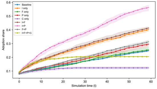
Figure 1. Dynamics of retrofit adoption across governance configurations. Lines report median adoption shares across simulation runs, with shaded bands indicating the interquartile range (IQR).

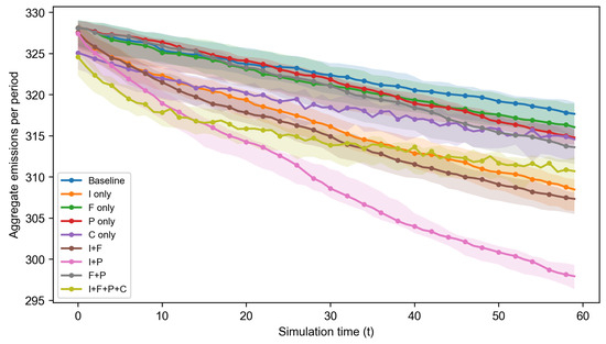
Figure 2. Evolution of aggregate neighbourhood emissions under alternative governance configurations. Median trajectories and interquartile ranges (IQR) are reported across stochastic simulations.

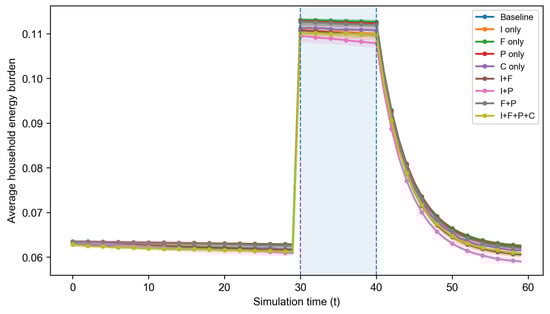
Figure 3. Average household energy burden over time across governance configurations. Solid lines represent median outcomes, with shaded areas denoting the interquartile range (IQR). Vertical dashed lines indicate the exogenous energy price shock window.

4.1. Adoption Dynamics

Figure 1 shows pronounced differences in retrofit diffusion across governance configurations. In scenarios without participatory coordination, adoption rises gradually and does not exhibit an early take-off. Incentives accelerate uptake relative to the baseline, whereas feedback alone remains close to the baseline trajectory over the horizon.

By contrast, configurations that include participation generate a strong early adoption pulse followed by tapering as the pool of remaining non-adopters shrinks. This pattern translates into substantially higher end-of-horizon adoption for participation-centred mixes. Consistent with Figure 1, the highest adoption share at $t=T-1$ occurs under the I+P configuration (I1F0P1C0; Table 2). Notably, the full instrument bundle (I+F+P+C) reaches a lower adoption plateau than I+P, indicating that adding compliance to an incentive–participation regime can dampen voluntary adoption in this setup.

To further characterise the diffusion process underlying these trajectories (not shown for brevity), we examined the implied inflow of new adopters over time. Participation-based configurations generate the strongest early uptake pulse, followed by rapid tapering; incentive-based configurations also exhibit an early uptake pulse, but less pronounced than participation-centred mixes. Baseline-like and feedback-only scenarios diffuse more gradually. These stock–flow differences help explain the timing of downstream environmental and social outcomes.

4.2. Environmental Outcomes

Figure 2 reports the aggregate neighbourhood emissions per period over time. All the policy scenarios reduce emissions relative to the baseline, but the magnitude and timing of reductions differ. Participation-centred configurations achieve the largest and earliest emission reductions, consistent with their rapid adoption dynamics.

Endpoint comparisons in Table 2 corroborate this ordering: I+P attains the lowest emissions at $t=T-1$, followed by incentive-based mixes, whereas the baseline and feedback-only scenarios cluster at higher endpoint emissions. Compliance-only governance reduces emissions relative to the baseline but does not match the reductions achieved by participation-based regimes.

4.3. Social Sustainability Outcomes

Social sustainability outcomes are assessed using the average household energy burden and its distribution. Figure 3 shows the trajectory of the average household energy burden over time, including the exogenous energy price shock window. Scenarios with higher adoption generally exhibit lower mean burden trajectories both before and after the shock. Participation-based configurations (especially when paired with incentives) display the lowest mean burden trajectories over the horizon, whereas baseline-like and low-adoption configurations exhibit higher burden levels.

Distributional outcomes are not monotonic in adoption intensity. At the simulation endpoint, Figure 4 illustrates an emissions–inequality trade-off: compliance-only governance yields the lowest burden inequality (Gini), whereas the configuration that minimises emissions (I+P) exhibits comparatively higher inequality despite a lower mean burden. The full bundle (I+F+P+C) shifts outcomes along this trade-off: relative to I+P, it improves inequality but does not outperform I+P in terms of adoption or aggregate emissions in the baseline runs (Table 2). This highlights that adding instruments can generate distributional gains without improving diffusion or mitigation outcomes.

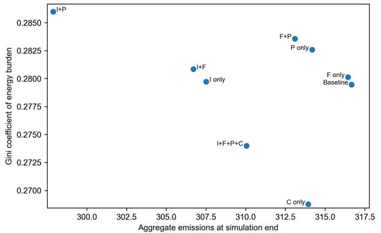
Figure 4. Trade-off between aggregate emissions and inequality in household energy burden at the simulation endpoint. Each point represents a governance configuration, labelled by its policy mix.

4.4. Resilience to Energy Price Shocks

An exogenous energy price shock induces a sharp increase in the household energy burden across all governance configurations (Figure 3). Table 3 summarises the neighbourhood-level burden responses to the shock, reporting the pre-shock burden, peak burden during the shock window, overshoot magnitude, recovery time, and post-shock volatility. The main cross-scenario differences appear in relation to peak and overshoot magnitudes rather than to recovery speed. Participation-centred configurations experience smaller burden peaks and overshoots, whereas baseline-like configurations exhibit larger increases. Post-shock adjustment paths are broadly similar across governance mixes, with recovery times relatively close across scenarios (Table 3).

4.5. Fiscal Feasibility

Figure 4 illustrates the trade-off between aggregate emissions and inequality in household energy burden at the simulation endpoint. Figure 5 compares the cumulative net public budget costs across governance configurations. The public budget cost is reported as the incremental net fiscal exposure of policy instruments (administration + subsidies + enforcement minus fine revenues) and is therefore interpreted as a feasibility benchmark rather than a welfare-optimal objective.

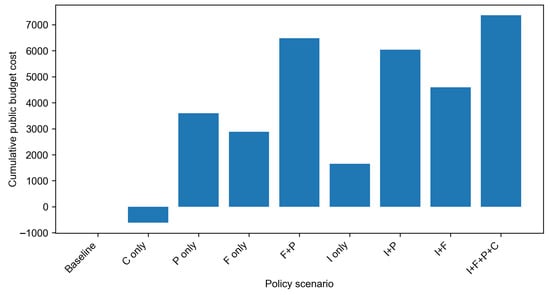
Figure 5. Cumulative net public budget cost associated with alternative governance configurations over the full simulation horizon.

Incentive-only and feedback-only governance entail relatively low fiscal exposure, while participation-based configurations involve higher administrative costs. Compliance-based governance incurs enforcement expenditure that can be partially offset by fine revenues, which may yield negative net values under the accounting definition. The full policy bundle (I+F+P+C) entails the highest cumulative net public cost and primarily shifts outcomes along the emissions–inequality trade-off: relative to I+P, it improves distributional inequality but does not outperform I+P in relation to adoption or aggregate emissions in the baseline runs (Table 2). This highlights that adding compliance to an incentive–participation regime can be fiscally expensive while yielding benefits concentrated in distributional rather than diffusion or mitigation metrics.

Table 2 provides a comparative overview of environmental, social, and fiscal outcomes across governance configurations, highlighting systematic differences in the end-of-horizon adoption shares, endpoint emissions, distributional impacts, and cumulative net public cost.

4.6. Robustness Under Parameter Uncertainty: Global Sensitivity and Rank Stability

To evaluate whether the relative ordering of governance configurations is robust to joint parameter uncertainty, we conduct a global sensitivity (rank stability) exercise across 200 joint parameter draws. For each draw, we record which scenario attains the best performance for each outcome (highest adoption; lowest total emissions, burden inequality, and cumulative net public cost). Table 4 summarises the winner frequency (top-1 counts). Overall, the evidence indicates that the main qualitative conclusions are not an artefact of a single parameterisation: participation-centred mixes dominate winner counts for adoption and frequently appear among the top performers in terms of emissions.

Table 4. Rank stability winner frequency under global sensitivity (200 parameter draws).

Metric	Winner Scenario	Count	Share (%)
Environmental outcome (lower is better)
Total emissions	I1F0P1C0	108	54.0
	I1F1P1C1	55	27.5
	I0F1P1C0	11	5.5
	I0F0P1C0	8	4.0
	I1F1P0C0	8	4.0
	I0F0P0C1	6	3.0
	I1F0P0C0	4	2.0
Adoption outcome (higher is better)
Adoption rate	I1F0P1C0	181	90.5
	I0F0P1C0	9	4.5
	I1F0P0C0	7	3.5
	I0F1P1C0	3	1.5
Fiscal outcome (lower is better; feasibility benchmark)
Cumulative net public cost	I0F0P0C0	182	91.0
	I0F0P0C1	18	9.0
Social outcome (lower is better)
Energy burden inequality (Gini)	I1F0P1C0	77	38.5
	I1F1P1C1	49	24.5
	I0F0P0C1	35	17.5
	I0F1P1C0	11	5.5
	I1F1P0C0	9	4.5
	I1F0P0C0	8	4.0
	I0F0P1C0	7	3.5
	I0F1P0C1	4	2.0

Note: For each draw, the “winner” is the policy scenario that performs best on the target metric (lower is better for emissions, inequality, and budget cost; higher is better for adoption). Policy scenarios are encoded as I#F#P#C#. Fiscal outcomes are interpreted as a feasibility benchmark rather than a normative top-1 objective; hence, they should be read alongside the full scenario summary (Table 2) and cost comparison (Figure 5).

By contrast, distributional rankings are more contested: different configurations emerge as winners for inequality under joint uncertainty, consistent with the trade-off structure shown in Figure 4. Fiscal outcomes are interpreted as a feasibility benchmark rather than a normative top-1 objective and should be read alongside Table 2 and Figure 5.

5. Discussion

5.1. Governance Mixes Structure Diffusion Pathways

The results indicate that neighbourhood energy transitions are shaped less by the intensity of any single instrument than by how governance mixes reconfigure the diffusion pathway through which adoption unfolds. Endpoint adoption shares are closely tied to distinct time profiles (Figure 1), implying that governance design has first-order consequences for coordination, timing, and path dependence rather than only for long run levels. This underscores the importance of policy mix evaluation, because single-lever assessments can misstate both distributional consequences and fiscal implementability in bundled neighbourhood programmes [16,39].

Participation-centred governance induces a coordinated diffusion pathway characterised by rapid take-off and accelerated convergence. Mechanistically, when local adoption exposure rises relative to the coordination threshold in the model, participation amplifies uptake through social coordination and expectation alignment, generating the steep early climb in adoption and the higher plateau observed for participation-based mixes (Figure 1). In this regime, adoption is not reducible to an accumulation of independent household choices; rather, collective dynamics (coordination, mutual updating, and synchronised timing) endogenously reshape perceived payoffs and accelerate convergence. Consistent with this pathway logic, the incentive–participation mix (I+P) attains the highest endpoint adoption and the lowest endpoint emissions in the baseline runs (Table 2).

In contrast, incentive- and feedback-based governance produces a more incremental diffusion pathway. Here, instruments primarily lower financial and informational barriers without creating strong endogenous coordination. Adoption therefore proceeds more gradually and heterogeneously across households, consistent with smoother adoption trajectories and lower endpoints relative to participation-centred mixes (Figure 1). Importantly, this is not a claim that incentives or feedback are ineffective; rather, their primary effect in the model is to shift individual thresholds without generating the self-reinforcing acceleration characteristic of coordinated regimes.

Compliance-based governance operates through a constraint-driven pathway. By increasing the expected cost of non-adoption or non-compliance, enforcement can reduce energy use even when voluntary uptake remains limited. At the same time, the availability of enforcement-driven reduction channels can dampen voluntary retrofit incentives for some households, contributing to weaker voluntary diffusion in compliance scenarios (Figure 1) while still delivering emission reductions (Figure 2) [47,48]. These mechanism interpretations are conditional on the behavioural rules, network interactions, and instrument implementations specified in the model (Appendix A).

A notable pattern in Figure 1 is that adding compliance to an already coordination-capable mix does not necessarily increase voluntary adoption. In the model, this “crowding out” effect arises through three linked mechanisms. First, enforcement and fines interact with household balance sheet constraints: when fines are paid out of wealth (or borrowed against limited debt headroom), they reduce the liquidity available for the upfront retrofit cost in subsequent periods, pushing marginal households below the feasibility threshold for adoption. Second, the compliance channel partially substitutes for voluntary efficiency upgrades by reducing the realised energy use among non-adopters through minimum-standard enforcement; when households anticipate that a fraction of savings can be achieved via enforcement, the relative incremental payoff from self-funded adoption narrows. Third, these two effects can disrupt coordination dynamics in participation-enabled regimes: by delaying adoption among would-be early followers, compliance pressure can slow the rise of local exposure above the collective action threshold, weakening the self-reinforcing take-off that otherwise characterises coordinated diffusion. Importantly, this mechanism is conditional: it is most likely when enforcement is salient early, when fines materially affect household budgets, and when coordination requires a critical mass of early adopters rather than purely individual optimisation. Accordingly, crowding out is most visible when compliance is layered onto mixes that would otherwise achieve take-off through coordination (e.g., participation-enabled regimes), rather than when diffusion is purely incremental.

The global sensitivity and rank stability evidence (Table 4) supports two robustness implications. First, participation-centred mixes are consistently top-ranked for adoption performance under joint parameter uncertainty, indicating that the coordinated pathway is not an artefact of a single calibration. Second, emission performance is more distributed across top-performing mixes, with I+P most frequently emerging as the best performer and the full bundle also appearing as a recurrent winner under joint uncertainty. Together, these results reinforce the view that governance instruments are pathway configuring rather than being interchangeable levers with purely additive effects. This contrast in rank stability naturally maps onto policy staging: adoption-oriented priorities are robust enough to guide early-phase instrument choice, whereas equity-oriented priorities require later-phase, context-sensitive calibration.

5.2. Social Sustainability Follows Diffusion Structure and Sequencing

A second implication is that social sustainability at the neighbourhood scale is driven by diffusion structure and sequencing, not merely by aggregate energy savings. In the model, governance mixes that achieve higher adoption coverage earlier tend to exhibit lower average energy burden trajectories (Figure 3) and slightly smaller shock peaks and overshoots (Table 3). Conceptually, this highlights that distributional outcomes are an emergent property of when different households access efficiency gains and how policy alters the outside option during transition periods, not only whether they adopt by the end of the horizon [24].

Under participation-centred governance, earlier coordination enables broader inclusion in efficiency gains within a shorter window, lowering average burden both pre- and post-shock (Figure 3). In this sense, participation functions as a timing alignment mechanism that reduces the duration for which late adopters remain exposed to higher costs, thereby lowering cumulative exposure to energy price risk.

However, high adoption does not mechanically translate into the lowest inequality. In the baseline runs, the compliance-only configuration yields the lowest burden inequality (Gini) even though it has relatively low voluntary adoption (Figure 4; Table 2). This can arise because enforcement compresses realised consumption (and therefore measured burden dispersion) without expanding voluntary retrofit access, indicating that distributional compression and inclusive uptake can represent distinct equity pathways. Importantly, this improvement refers to dispersion in energy burden (Gini of burden) and should not be interpreted as a comprehensive welfare or justice assessment.

This dual-pathway interpretation helps explain why distributional “winners” shift under joint parameter uncertainty. When uncertainty favours inclusive uptake (e.g., stronger means-tested support, looser credit constraints, or steeper coordination effects), equity improvements tend to be driven by wider and earlier access to retrofit gains, making participation-augmented mixes more likely to dominate social indicators. When uncertainty instead strengthens dispersion–compression dynamics (e.g., tighter standards, higher enforcement intensity, or more targeted enforcement exposure), burden inequality can fall even with limited voluntary adoption because realised consumption is compressed among non-adopters. In this sense, the sensitivity results do not undermine the model; they indicate regime-dependent dominance across equity pathways. A more credible implication is therefore a “winner set” rather than a single universally optimal design: policy makers should expect the equity-optimal instrument to depend on local financing capacity, enforcement feasibility, and the relative priority placed on inclusive uptake versus dispersion reduction. Practically, this suggests reporting the top-performing set (e.g., top three by frequency) and treating equity-optimal choices as scenario contingent rather than deterministic.

The shock analysis further underscores the role of sequencing. Configurations that achieve higher pre-shock adoption coverage tend to experience slightly smaller burden peaks and overshoots during the price shock window (Table 3). Notably, recovery times are broadly similar across scenarios in this setup, implying that cross-scenario resilience differences are expressed primarily through exposure levels at the shock onset rather than through differential recovery speed under a common post-shock price normalisation process.

Rank stability results caution against over-interpreting distributional “winners”. Unlike adoption, social metrics display more contested top-1 performance under joint uncertainty (Table 4), with I+P, the full bundle, and compliance-only governance each appearing as frequent winners across draws. This pattern suggests that distributional outcomes are more sensitive to joint parameter variation and reflect trade-off-dependent dominance rather than a single universally superior design.

5.3. Fiscal Feasibility and Institutional Sustainability of Governance Mixes

Fiscal feasibility emerges as a binding constraint on neighbourhood-scale governance, but it is best interpreted as a feasibility benchmark rather than an optimisation objective. Here, the public budget cost is defined as the incremental net fiscal exposure of policy instruments, computed as administration + subsidies + enforcement expenditures − fine revenues, summed over time (Table 2). This accounting measure captures programme budget requirements and implementability constraints rather than social welfare or total economic cost. Negative values, if any, indicate net fiscal revenue under this definition rather than negative programme spending. This should be read as an accounting exposure measure rather than a social surplus: fine revenues offset programme budgets in this metric but do not imply positive welfare effects.

A key distinction is between front-loaded and persistent fiscal burdens. Participation-centred governance entails higher administrative expenditure during early diffusion stages, reflecting the costs of facilitation and coordination, but these costs stabilise as adoption converges. By contrast, compliance-based governance can generate continuing enforcement and administrative demands across the horizon, even when marginal gains in voluntary adoption diminish. This difference matters for institutional sustainability: persistent enforcement can be difficult to finance and maintain, particularly under capacity constraints.

The full policy mix combining all instruments produces the highest cumulative net public cost and primarily reallocates performance across dimensions rather than dominating them: relative to I+P, it improves distributional inequality but does not outperform I+P in relation to adoption or emissions in the baseline runs (Figure 4 and Figure 5; Table 2). This pattern is consistent with diminishing returns once coordinated diffusion has already been triggered, and with the possibility that compliance pressure can reduce voluntary uptake when enforcement provides an alternative pathway to energy reduction. From a design perspective, the results imply that policy packages should be staged to match diffusion phases: early-stage resources may be better allocated to mechanisms that unlock coordination and accelerate take-off, while later-stage escalation through layered instruments may be justified primarily when distributional or compliance objectives are prioritised, given their fiscal and administrative demands [17,30].

To translate these conditional results into implementable guidance, the model suggests a phase-matched sequencing of instruments (Figure 6). Phase 1: Triggering Take-Off: Prioritise participation-enabled coordination with targeted incentives (P + means-tested I) to push local exposure above the collective threshold and accelerate early diffusion; monitor early-flow indicators such as the new adopter rate and adoption clustering to verify that take-off has been triggered. Phase 2: Scaling and Stabilisation: Once adoption is on a clear upward trajectory, add feedback (F) to reduce informational noise and perceived frictions, improving decision certainty and lowering heterogeneity in uptake; monitor reductions in burden volatility and the closing of the high–low adoption gap. Phase 3: Late-Stage Equity and Compliance Backstop: When adoption approaches a plateau and remaining households are “hard-to-adopt” due to financing or hassle constraints, introduce calibrated compliance measures (soft C; e.g., gradual standard ramping and capacity-bounded enforcement, paired with means-tested support to avoid liquidity shocks) primarily to address minimum-standard outcomes and distributional objectives; additionally, monitor overburden prevalence, burden inequality, and the policy compliance rate while tracking cumulative administrative and enforcement costs as institutional constraints. This staging logic preserves the benefits of coordinated diffusion while reducing the risk that early compliance pressure crowds out voluntary adoption in coordination-capable mixes.

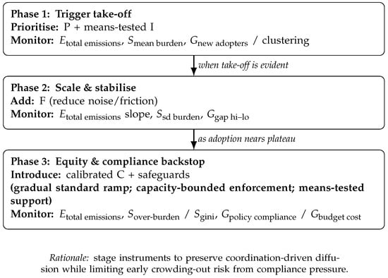
Figure 6. A phase-matched ESG implementation roadmap translating the model’s conditional findings into actionable sequencing and monitoring signals (E: emissions; S: energy-burden outcomes; and G: diffusion and governance feasibility).

Taken together, these findings underscore that institutional sustainability depends on aligning governance design with both diffusion dynamics and fiscal capacity. Governance mixes that catalyse early coordination can deliver strong mitigation and burden reductions without requiring continuous enforcement escalation, whereas compliance-heavy designs can achieve distributional compression at a higher administrative cost and potentially lower voluntary legitimacy. These conclusions remain conditioned on the behavioural rules, network structure, and policy implementations specified in the model (Appendix A); the rank stability analysis provides reassurance that the main qualitative ordering for diffusion is not driven by a single calibration, while distributional rankings are comparatively more sensitive under joint uncertainty.

6. Conclusions

This study develops an agent-based modelling framework to examine how alternative governance mixes shape neighbourhood-scale building energy transitions when diffusion dynamics, social sustainability, and fiscal feasibility are considered jointly. Modelling heterogeneous households embedded in social networks allows us to trace how behavioural responses and policy instruments interact to produce aggregate environmental and distributional outcomes over time.

Three conclusions follow. First, governance mixes primarily restructure diffusion pathways. Participation-centred configurations generate rapid, coordinated take-off and early convergence, whereas incentive- and feedback-based approaches diffuse more incrementally. Compliance-based governance can reduce energy use through enforcement, but does not generate comparable levels of voluntary retrofit adoption. Second, social sustainability follows a diffusion structure and sequencing, but not in a one-to-one way with adoption intensity: earlier and broader uptake is associated with lower average energy burden and modestly smaller shock peaks and overshoots, while inequality outcomes can also improve via enforcement-driven compression even when voluntary adoption is limited. Third, fiscal feasibility acts as a binding implementability constraint. Using an accounting definition of net public cost (administration + subsidies + enforcement − fine revenues), we find that the full bundle is the most expensive configuration and mainly trades fiscal resources for distributional improvement rather than dominating adoption or emissions relative to I+P.

Global sensitivity analysis confirms that the qualitative adoption advantage of participation-centred mixes is robust under joint parameter uncertainty, whereas distributional “winners” remain comparatively more sensitive across configurations. Overall, the results support evaluating neighbourhood retrofit governance as a portfolio design problem in which instruments configure diffusion pathways and redistribute performance across mitigation, equity, and feasibility dimensions.

Several limitations suggest priorities for future work. The model reports costs and household finances in normalised units rather than fully calibrated currency terms, and abstracts from richer building stock heterogeneity and potentially adaptive network structures. Empirical calibration, alternative targeting designs, heterogeneous enforcement capacity, and additional real-world frictions (e.g., transaction costs, supply constraints, or rebound effects) would help to map the equity–efficiency–feasibility trade-offs identified here to specific policy settings.

Appendix A.1. Purpose

The model examines how a bundle of governance levers—incentives (I), feedback (F), participation (P), and compliance (C)—interacts with household heterogeneity and neighbourhood social influence to shape (i) retrofit adoption dynamics (diffusion, clustering, and equity gaps), (ii) neighbourhood environmental outcomes (energy use and emissions), (iii) distributional social outcomes (energy affordability burden and inequality), and (iv) governance outcomes (policy compliance and public budget components), particularly under an exogenous energy price shock and recovery.

The model is designed for mechanism-based comparison across governance mixes rather than city-specific forecasting. The parameters are set within stylized, literature-consistent ranges and robustness is assessed through multi-seed summaries and global sensitivity ranges (Table A2 and Table A3). The baseline values in Table A2 and Table A3 correspond to the best-fitting calibration configuration used in the main experiments (see the configuration file in the reproducibility package).

Appendix A.2. Reproducibility Package

The reproducibility package includes (i) the full source code; (ii) a pinned environment specification; (iii) a baseline configuration file (calibration_best_cfg.json); (iv) scripts/notebooks to regenerate all figures and tables from raw simulation outputs; and (v) a README documenting command line usage, seed control, and output directories. All the stochastic components (initialization, belief noise, adoption draws, enforcement draws, and optional replacement window arrivals) are controlled by explicit random seeds; the reported results are summarized across multiple seeds using the median and IQR.

Appendix A.3. Entities, State Variables, and Scales

Entities. The model contains two entity types: (i) household agents $i=1,\dots ,N$, and (ii) a policy environment represented by $(I,F,P,C)\in {\{0,1\}}^4$ and an exogenous energy price process $p_t$.

Scales. Time is discrete, $t=0,1,\dots ,T-1$, with each step representing a fixed decision interval (normalized). The spatial setting is a stylized neighbourhood social network $G=(V,E)$ that is generated once per experiment set and held fixed across policy scenarios.

State variables. Each household is represented by the state vector

$${\mathbf{s}}_{i,t}=\{g_i,y_i,e_i^0,a_{i,t},b_{i,t},h_i,{\xi }_i,w_{i,t},d_{i,t},n_{i,t},r_{i,t},u_{i,t}^B,u_{i,t}^I\},$$

where $g_i$ is the income group, $y_i$ is income, $e_i^0$ is the baseline energy demand, $a_{i,t}$ is the adoption status, $b_{i,t}$ is the perceived proportional saving rate used in decision making, $h_i$ is the hassle/friction, ${\xi }_i$ is the idiosyncratic taste shock, $w_{i,t}$ is wealth, $d_{i,t}$ is debt, $n_{i,t}$ is the accumulated non-compliance count, $r_{i,t}$ is a replacement window timer (optional robustness module), and $u_{i,t}^B$/$u_{i,t}^I$ are cumulative bookkeeping counters recording how many times adoption required borrowing and how many times the installment (extra credit line) was used (auditing the financing/friction module).

The operational definitions, domains, initialization distributions, truncation/constraints, and time-variation are listed in Table A1.

Table A1. State variables: operationalization, initialization, and constraints (aligned with code).

Variable	Domain	Initialization (Distribution/Rule)	Dynamics/Constraints
Income group $g_i$	$\{0,1,2\}$	Categorical draw with shares $(0.35,0.45,0.20)$	Fixed
Income $y_i$	${\mathbb{R}}_{+}$	Group-specific levels $(1.0,1.8,3.0)$	Fixed; normalization uses $max(y_i,\underline{y})$ with $\underline{y}=0.5$
Baseline energy $e_i^0$	${\mathbb{R}}_{+}$	Truncated normal $\mathcal{N}({\mu }_E,{\sigma }_E)$, clipped to ≥0.15	Fixed baseline; realised energy depends on adoption/enforcement
Adoption $a_{i,t}$	$\{0,1\}$	Bernoulli early adopters (default $0.08$)	Irreversible: once 1, remains 1
Belief $b_{i,t}$	$[b_{min},b_{max}]$	Normal around ${\alpha }_E$, sd $s_b$, clipped to bounds	Updated by learning (Equation (A4)); clipped each step
Hassle $h_i$	${\mathbb{R}}_{+}$	Truncated normal, mean ${\mu }_h$, sd ${\sigma }_h$, clipped to ≥0	Fixed; scaled down under feedback by $(1-{\gamma }_F)$
Taste ${\xi }_i$	$\mathbb{R}$	Normal $\mathcal{N}(0,{\sigma }_{\xi })$	Fixed; enters friction term (can offset hassle)
Wealth $w_{i,t}$	${\mathbb{R}}_{+}$	Lognormal conditional on income (weak income–wealth elasticity)	Updated by income, consumption, bills, saving/repayment; constrained $w_{i,t}\ge 0$
Debt $d_{i,t}$	$[0,{\overline{d}}_i]$	$d_{i,0}=0$	Interest + repayment + borrowing; clamped to ${\overline{d}}_i=\chi y_i$ (Equation (A2))
Non-compliance count $n_{i,t}$	${\mathbb{Z}}_{\ge 0}$	$n_{i,0}=0$	Increments if non-adopting and not enforced; resets/decrements when adopted or enforced
Replacement timer $r_{i,t}$	${\mathbb{Z}}_{\ge 0}$	$r_{i,0}=0$	Optional: activated with prob. $p_{\mathrm{rep}}$; counts down if active
Borrow-use counter $u_{i,t}^B$	${\mathbb{Z}}_{\ge 0}$	0	Cumulative: $+1$ if adoption used borrowing in step t
Installment-use counter $u_{i,t}^I$	${\mathbb{Z}}_{\ge 0}$	0	Cumulative: $+1$ if installment line used (adds friction)

Table A1. State variables: operationalization, initialization, and constraints (aligned with code).

Variable	Domain	Initialization (Distribution/Rule)	Dynamics/Constraints
Income group $g_i$	$\{0,1,2\}$	Categorical draw with shares $(0.35,0.45,0.20)$	Fixed
Income $y_i$	${\mathbb{R}}_{+}$	Group-specific levels $(1.0,1.8,3.0)$	Fixed; normalization uses $max(y_i,\underline{y})$ with $\underline{y}=0.5$
Baseline energy $e_i^0$	${\mathbb{R}}_{+}$	Truncated normal $\mathcal{N}({\mu }_E,{\sigma }_E)$, clipped to ≥0.15	Fixed baseline; realised energy depends on adoption/enforcement
Adoption $a_{i,t}$	$\{0,1\}$	Bernoulli early adopters (default $0.08$)	Irreversible: once 1, remains 1
Belief $b_{i,t}$	$[b_{min},b_{max}]$	Normal around ${\alpha }_E$, sd $s_b$, clipped to bounds	Updated by learning (Equation (A4)); clipped each step
Hassle $h_i$	${\mathbb{R}}_{+}$	Truncated normal, mean ${\mu }_h$, sd ${\sigma }_h$, clipped to ≥0	Fixed; scaled down under feedback by $(1-{\gamma }_F)$
Taste ${\xi }_i$	$\mathbb{R}$	Normal $\mathcal{N}(0,{\sigma }_{\xi })$	Fixed; enters friction term (can offset hassle)
Wealth $w_{i,t}$	${\mathbb{R}}_{+}$	Lognormal conditional on income (weak income–wealth elasticity)	Updated by income, consumption, bills, saving/repayment; constrained $w_{i,t}\ge 0$
Debt $d_{i,t}$	$[0,{\overline{d}}_i]$	$d_{i,0}=0$	Interest + repayment + borrowing; clamped to ${\overline{d}}_i=\chi y_i$ (Equation (A2))
Non-compliance count $n_{i,t}$	${\mathbb{Z}}_{\ge 0}$	$n_{i,0}=0$	Increments if non-adopting and not enforced; resets/decrements when adopted or enforced
Replacement timer $r_{i,t}$	${\mathbb{Z}}_{\ge 0}$	$r_{i,0}=0$	Optional: activated with prob. $p_{\mathrm{rep}}$; counts down if active
Borrow-use counter $u_{i,t}^B$	${\mathbb{Z}}_{\ge 0}$	0	Cumulative: $+1$ if adoption used borrowing in step t
Installment-use counter $u_{i,t}^I$	${\mathbb{Z}}_{\ge 0}$	0	Cumulative: $+1$ if installment line used (adds friction)

Appendix A.4. Project Overview and Schedule

Each time step is executed in the following order to ensure consistent causal sequencing: (1) update the energy price $p_t$; (2) update the household cashflows (wealth/debt), bills, and repayment; (3) update the replacement window state (if enabled); (4) update beliefs $b_{i,t}$; (5) update the compliance standard $s_t$ (if $C=1$); (6) compute the adoption decisions subject to liquidity/credit constraints; (7) compute the realised energy and emissions; (8) draw enforcement and apply fines (if $C=1$); and (9) record the E/S/G outcomes and public budget components.

Algorithm A1 One simulation step t (aligned with code).

1: Compute energy price $p_t$ via Equation (A1). 2: for each household i do 3:       Accrue interest on debt; compute income inflow and essential consumption. 4:       Pay energy bill; update wealth $w_{i,t}$ by saving/repayment rules. 5:       Repay debt from surplus if possible; clamp debt to cap (Equation (A2)). 6: end for 7: if replacement window enabled then 8:       for each non-adopter i do 9:             With probability $p_{\mathrm{rep}}$, open a replacement window of duration $D_{\mathrm{rep}}$; decrement timer if active. 10:       end for 11: end if 12: for each household i do 13:       Update belief $b_{i,t}\to b_{i,t+1}$ using Equation (A4). 14: end for 15: if  $C=1$  then 16:       Update minimum standard $s_t$ via Equation  (9). 17: end if 18: for each non-adopter i do 19:       Check affordability/credit feasibility (base credit; optional installment line). 20:       Compute $\mathrm{\Delta }{U}_{i,t}$ (Equation  (16)) and draw adoption with logit rule (Equation  (17)). 21: end for 22: Compute realised energy and emissions (adoption + enforcement adjustments). 23: if  $C=1$  then 24:       Draw enforcement among non-adopters subject to capacity and income-targeted probabilities. 25:       Apply enforced reduction and fines; update non-compliance count $n_{i,t}$; record fine collection/unpaid. 26: end if 27: Record E/S/G outcomes and public budget components.

Appendix A.5. Design Concepts

• Heterogeneity. Households differ by income group/income, baseline energy demand, initial wealth, behavioural friction, taste, and beliefs about savings (Table A1).
• Bounded rationality and stochastic choice. Adoption follows a quantal response (logit) rule with decision temperature $T_{\mathrm{dec}}$. When feedback is active, the temperature is reduced by a fractional amount ${\delta }_T$, increasing decision certainty.
• Learning and information. Beliefs about savings update from noisy local social signals. When feedback is active, the perceived signal is anchored to a benchmark, updated with a higher learning rate, and subject to lower noise.
• Social influence and coordination. Neighbour adoption exposure affects utility. Participation activates a coordination function ${\kappa }_{i,t}$ that strengthens social influence and unlocks collective cost reductions and group buy discounts once the local adoption exceeds a threshold.
• Constraints and financing. Adoption must satisfy liquidity/credit constraints. Debt is bounded by an income-proportional hard cap. Optional installment financing extends the effective credit line (with a low-income boost) but adds an extra friction penalty if used.
• Stochasticity and replication. Randomness enters through initialization, belief noise, adoption draws, enforcement draws, and replacement window arrivals. The results are summarized across multiple seeds using the median and interquartile range (IQR).

Appendix A.6. Initialization

At $t=0$, households are assigned income groups by categorical shares; incomes take group-specific levels. The baseline energy demand is drawn from a truncated normal distribution and clipped to ensure positivity. A small share of early adopters is initialized. Beliefs are drawn around the technical savings parameter ${\alpha }_E$ and clipped to $[b_{min},b_{max}]$. Hassle and taste are drawn from parametric distributions; wealth is initialized from a lognormal distribution conditional on income; debt and non-compliance are initialized at zero; and bookkeeping counters are initialized at zero. The network is generated once and held fixed across policy scenarios within each experiment set.

Table A2. Baseline parameters and tested ranges (aligned with code; baseline values correspond to calibration_best_cfg.json; rounded for readability). Part A: population, network, energy/price shock, beliefs/choice, social influence, and incentives.

Parameter	Symbol	Baseline	Role/Where Used	Range Tested
Number of households	N	600	Population size	Fixed
Simulation steps	T	60	Horizon length	Fixed
Degree (ring lattice)	k	10	Network degree	6–14 (even)
Swap intensity (double-edge swaps)	p	0.08	Degree-preserving rewiring intensity	0.00–0.20
Baseline energy mean	${\mu }_E$	1.00	Init $e_i^0$ mean	0.8–1.2
Baseline energy sd	${\sigma }_E$	0.25	Init $e_i^0$ sd	0.15–0.35
Upfront adoption cost (base)	$C_0$	3.59	Cost before policy reductions	1.0–3.5
Energy reduction rate (technical)	${\alpha }_E$	0.185	Post-adoption energy reduction	0.08–0.25
Energy unit price (base)	$p_0$	0.096	Price per unit energy	0.08–0.20
Shock step	$t_s$	30	Shock timing (step index)	Fixed
Shock multiplier	m	1.8	Shock severity	1.2–2.5
Shock duration	$\mathrm{\Delta }t$	10	Shock length (steps)	5–15
Recovery constant	${\tau }_s$	4.0	Exponential recovery speed	2–8
Floor multiplier	$m_{min}$	1.0	Post-shock floor	0.8–1.2
Beliefs/feedback (F)
Learning rate (base)	${\lambda }_0$	0.10	Belief updating	0.05–0.25
Learning boost (F)	$\mathrm{\Delta }\lambda$	0.16	Additional learning under feedback	0.05–0.25
Signal noise sd (no F)	${\sigma }_{\epsilon }$	0.10	Noise in belief signal	0.05–0.20
Signal noise sd (F)	${\sigma }_{\epsilon ,F}$	0.05	Reduced noise under feedback	0.02–0.10
Peer/benchmark blend weight (F)	${\omega }_s$	0.55	Weight on peer signal when $F=1$	Fixed (code constant)
Belief init sd	$s_b$	0.12	Init dispersion for $b_{i,0}$	Fixed
Belief bounds	$(b_{min},b_{max})$	(0.02, 0.60)	Clipping interval for $b_{i,t}$	Fixed
Choice/bounded rationality
Decision temperature (base)	$T_{\mathrm{dec}}$	0.900	Logit choice noise	0.4–1.6
Temperature reduction (F)	${\delta }_T$	0.15	Fractional reduction when $F=1$	0.05–0.30
Social influence/participation (P)
Social weight (base)	${\omega }_0$	1.00	Baseline social influence weight	0.3–1.5
Social weight boost (P)	${\delta }_{\omega }$	0.25	Coordination-based social amplification	0.10–0.60
Neighbour sample size	$n_s$	10	Sample size for ${\overline{a}}_{{\mathcal{N}}_i,t}$	Fixed
Coordination threshold	$\theta$	0.35	Threshold in Equation  (8)	0.22–0.45
Coordination steepness	$\eta$	10.0	Steepness in Equation (8)	8–20
Participation cost (per step)	$c_P$	0.01	Participation overhead when $P=1$	0.00–0.03
Coordination cost reduction	${\delta }_C$	0.10	Cost reduction unlocked by ${\kappa }_{i,t}$	0.05–0.25
Group buy discount	${\delta }_G$	0.20	Extra discount unlocked by ${\kappa }_{i,t}$	Fixed (code constant)
Group buy social add-on	${\omega }_G$	0.25	Extra social term under ${\kappa }_{i,t}$	Fixed (code constant)
Incentives (I)
Subsidy rate	$\sigma$	0.25	Upfront cost reduction under incentives	0.10–0.50
Means test strength	${\tau }_I$	0.345	Increases subsidy for low income	Fixed (baseline)
Low-income credit boost	${\beta }_I$	0.216	Boosts installment line for low income	Fixed (baseline)

Table A2. Baseline parameters and tested ranges (aligned with code; baseline values correspond to calibration_best_cfg.json; rounded for readability). Part A: population, network, energy/price shock, beliefs/choice, social influence, and incentives.

Parameter	Symbol	Baseline	Role/Where Used	Range Tested
Number of households	N	600	Population size	Fixed
Simulation steps	T	60	Horizon length	Fixed
Degree (ring lattice)	k	10	Network degree	6–14 (even)
Swap intensity (double-edge swaps)	p	0.08	Degree-preserving rewiring intensity	0.00–0.20
Baseline energy mean	${\mu }_E$	1.00	Init $e_i^0$ mean	0.8–1.2
Baseline energy sd	${\sigma }_E$	0.25	Init $e_i^0$ sd	0.15–0.35
Upfront adoption cost (base)	$C_0$	3.59	Cost before policy reductions	1.0–3.5
Energy reduction rate (technical)	${\alpha }_E$	0.185	Post-adoption energy reduction	0.08–0.25
Energy unit price (base)	$p_0$	0.096	Price per unit energy	0.08–0.20
Shock step	$t_s$	30	Shock timing (step index)	Fixed
Shock multiplier	m	1.8	Shock severity	1.2–2.5
Shock duration	$\mathrm{\Delta }t$	10	Shock length (steps)	5–15
Recovery constant	${\tau }_s$	4.0	Exponential recovery speed	2–8
Floor multiplier	$m_{min}$	1.0	Post-shock floor	0.8–1.2
Beliefs/feedback (F)
Learning rate (base)	${\lambda }_0$	0.10	Belief updating	0.05–0.25
Learning boost (F)	$\mathrm{\Delta }\lambda$	0.16	Additional learning under feedback	0.05–0.25
Signal noise sd (no F)	${\sigma }_{\epsilon }$	0.10	Noise in belief signal	0.05–0.20
Signal noise sd (F)	${\sigma }_{\epsilon ,F}$	0.05	Reduced noise under feedback	0.02–0.10
Peer/benchmark blend weight (F)	${\omega }_s$	0.55	Weight on peer signal when $F=1$	Fixed (code constant)
Belief init sd	$s_b$	0.12	Init dispersion for $b_{i,0}$	Fixed
Belief bounds	$(b_{min},b_{max})$	(0.02, 0.60)	Clipping interval for $b_{i,t}$	Fixed
Choice/bounded rationality
Decision temperature (base)	$T_{\mathrm{dec}}$	0.900	Logit choice noise	0.4–1.6
Temperature reduction (F)	${\delta }_T$	0.15	Fractional reduction when $F=1$	0.05–0.30
Social influence/participation (P)
Social weight (base)	${\omega }_0$	1.00	Baseline social influence weight	0.3–1.5
Social weight boost (P)	${\delta }_{\omega }$	0.25	Coordination-based social amplification	0.10–0.60
Neighbour sample size	$n_s$	10	Sample size for ${\overline{a}}_{{\mathcal{N}}_i,t}$	Fixed
Coordination threshold	$\theta$	0.35	Threshold in Equation  (8)	0.22–0.45
Coordination steepness	$\eta$	10.0	Steepness in Equation (8)	8–20
Participation cost (per step)	$c_P$	0.01	Participation overhead when $P=1$	0.00–0.03
Coordination cost reduction	${\delta }_C$	0.10	Cost reduction unlocked by ${\kappa }_{i,t}$	0.05–0.25
Group buy discount	${\delta }_G$	0.20	Extra discount unlocked by ${\kappa }_{i,t}$	Fixed (code constant)
Group buy social add-on	${\omega }_G$	0.25	Extra social term under ${\kappa }_{i,t}$	Fixed (code constant)
Incentives (I)
Subsidy rate	$\sigma$	0.25	Upfront cost reduction under incentives	0.10–0.50
Means test strength	${\tau }_I$	0.345	Increases subsidy for low income	Fixed (baseline)
Low-income credit boost	${\beta }_I$	0.216	Boosts installment line for low income	Fixed (baseline)

Table A3. Baseline parameters and tested ranges (aligned with code; baseline values correspond to calibration_best_cfg.json; rounded for readability). Part B: frictions, debt/cashflow, compliance, NPV perception, optional modules, and constants.

Parameter	Symbol	Baseline	Role/Where Used	Range Tested
Adoption frictions (heterogeneity)
Hassle mean	${\mu }_h$	0.602	Mean hassle $h_i$	0.18–0.70
Hassle sd	${\sigma }_h$	0.08	Dispersion of $h_i$	0.05–0.12
Taste sd	${\sigma }_{\xi }$	0.10	Dispersion of ${\xi }_i$	0.06–0.14
Hassle reduction (F)	${\gamma }_F$	0.30	Fractional hassle reduction when $F=1$	0.15–0.40
Installment friction	${\varphi }_{\mathrm{inst}}$	0.05	Extra friction if installment used	Fixed
Debt/cashflow dynamics
Income flow per step	$\upsilon$	0.12	Income inflow each step (scaled by $y_i$)	Fixed
Consumption share	${\kappa }_c$	0.70	Essential consumption share of income flow	Fixed
Base saving rate	${\kappa }_s$	0.10	Saving share of positive disposable	Fixed
Saving boost (F)	${\delta }_s$	0.06	Extra saving under feedback	Fixed
Base credit ratio	${\chi }_0$	0.096	Base credit line $d_i^{\mathrm{base}}={\chi }_0{y}_i$	Fixed (baseline)
Hard debt cap ratio	$\chi$	1.021	Hard cap $d_{i,t}\in [0,\chi y_i]$	Fixed (baseline)
Debt interest rate	$r_d$	0.01	Interest accrual on debt (per step)	Fixed
Repayment share	${\pi }_d$	0.35	Share of surplus used to repay debt	Fixed
Installment extra credit ratio	${\chi }_{\mathrm{inst}}$	0.35	Extra credit line under installment	Fixed (baseline)
Compliance/enforcement (C)
Penalty pressure (base)	${\mathrm{\Pi }}_0$	0.10	Outside option pressure when $C=1$	0.05–0.20
Penalty escalation	${\alpha }_{\mathrm{\Pi }}$	0.015	Escalation with $n_{i,t}$	Fixed
Standard base	$s_0$	0.03	Initial minimum standard	0.00–0.05
Standard ramp	$\rho$	0.0015	Tightening rate	0.001–0.004
Standard max	$\overline{s}$	0.14	Upper bound for standard	0.10–0.25
Enforcement probability (base)	$p_e$	0.25	Enforcement draw under compliance	0.10–0.60
Enforcement strength	$\psi$	1.0	Strength of enforced reduction	Fixed
Fine per violation	f	0.08	Fine assessed for non-compliance	0.03–0.15
Enforcement targeting bias	${\beta }_C$	0.4	Higher enforcement prob for low income	Fixed
Enforcement capacity	${\mathrm{\Omega }}_C$	1.0	Scales enforcement probability	Fixed
NPV perception (F)
NPV horizon (base)	$H_0$	12	Discounted horizon when $F=0$	Fixed (baseline)
NPV horizon (F)	$H_F$	18	Discounted horizon when $F=1$	Fixed (baseline)
NPV discount (base)	$r_0$	0.03	Discount rate when $F=0$	Fixed (baseline)
NPV discount (F)	$r_F$	0.02	Discount rate when $F=1$	Fixed (baseline)
Optional modules
Installment financing enabled	—	True	Enables extra credit line + friction	Fixed (baseline)
Replacement window enabled	—	True	Temporary cost discount	Fixed (baseline)
Replacement prob. (per step)	$p_{\mathrm{rep}}$	0.012	Window arrival prob. for non-adopters	0.00–0.03
Replacement discount	${\delta }_{\mathrm{rep}}$	0.55	Cost discount when window active	0.20–0.70
Replacement duration	$D_{\mathrm{rep}}$	3	Steps window remains active	2–6
Emissions factor	${\varphi }_{{\mathrm{CO}}_2}$	0.55	Converts energy to emissions	Fixed
Affordability threshold	$\overline{B}$	0.10	Overburden rule $B_{i,t}>\overline{B}$	Fixed

Table A3. Baseline parameters and tested ranges (aligned with code; baseline values correspond to calibration_best_cfg.json; rounded for readability). Part B: frictions, debt/cashflow, compliance, NPV perception, optional modules, and constants.

Parameter	Symbol	Baseline	Role/Where Used	Range Tested
Adoption frictions (heterogeneity)
Hassle mean	${\mu }_h$	0.602	Mean hassle $h_i$	0.18–0.70
Hassle sd	${\sigma }_h$	0.08	Dispersion of $h_i$	0.05–0.12
Taste sd	${\sigma }_{\xi }$	0.10	Dispersion of ${\xi }_i$	0.06–0.14
Hassle reduction (F)	${\gamma }_F$	0.30	Fractional hassle reduction when $F=1$	0.15–0.40
Installment friction	${\varphi }_{\mathrm{inst}}$	0.05	Extra friction if installment used	Fixed
Debt/cashflow dynamics
Income flow per step	$\upsilon$	0.12	Income inflow each step (scaled by $y_i$)	Fixed
Consumption share	${\kappa }_c$	0.70	Essential consumption share of income flow	Fixed
Base saving rate	${\kappa }_s$	0.10	Saving share of positive disposable	Fixed
Saving boost (F)	${\delta }_s$	0.06	Extra saving under feedback	Fixed
Base credit ratio	${\chi }_0$	0.096	Base credit line $d_i^{\mathrm{base}}={\chi }_0{y}_i$	Fixed (baseline)
Hard debt cap ratio	$\chi$	1.021	Hard cap $d_{i,t}\in [0,\chi y_i]$	Fixed (baseline)
Debt interest rate	$r_d$	0.01	Interest accrual on debt (per step)	Fixed
Repayment share	${\pi }_d$	0.35	Share of surplus used to repay debt	Fixed
Installment extra credit ratio	${\chi }_{\mathrm{inst}}$	0.35	Extra credit line under installment	Fixed (baseline)
Compliance/enforcement (C)
Penalty pressure (base)	${\mathrm{\Pi }}_0$	0.10	Outside option pressure when $C=1$	0.05–0.20
Penalty escalation	${\alpha }_{\mathrm{\Pi }}$	0.015	Escalation with $n_{i,t}$	Fixed
Standard base	$s_0$	0.03	Initial minimum standard	0.00–0.05
Standard ramp	$\rho$	0.0015	Tightening rate	0.001–0.004
Standard max	$\overline{s}$	0.14	Upper bound for standard	0.10–0.25
Enforcement probability (base)	$p_e$	0.25	Enforcement draw under compliance	0.10–0.60
Enforcement strength	$\psi$	1.0	Strength of enforced reduction	Fixed
Fine per violation	f	0.08	Fine assessed for non-compliance	0.03–0.15
Enforcement targeting bias	${\beta }_C$	0.4	Higher enforcement prob for low income	Fixed
Enforcement capacity	${\mathrm{\Omega }}_C$	1.0	Scales enforcement probability	Fixed
NPV perception (F)
NPV horizon (base)	$H_0$	12	Discounted horizon when $F=0$	Fixed (baseline)
NPV horizon (F)	$H_F$	18	Discounted horizon when $F=1$	Fixed (baseline)
NPV discount (base)	$r_0$	0.03	Discount rate when $F=0$	Fixed (baseline)
NPV discount (F)	$r_F$	0.02	Discount rate when $F=1$	Fixed (baseline)
Optional modules
Installment financing enabled	—	True	Enables extra credit line + friction	Fixed (baseline)
Replacement window enabled	—	True	Temporary cost discount	Fixed (baseline)
Replacement prob. (per step)	$p_{\mathrm{rep}}$	0.012	Window arrival prob. for non-adopters	0.00–0.03
Replacement discount	${\delta }_{\mathrm{rep}}$	0.55	Cost discount when window active	0.20–0.70
Replacement duration	$D_{\mathrm{rep}}$	3	Steps window remains active	2–6
Emissions factor	${\varphi }_{{\mathrm{CO}}_2}$	0.55	Converts energy to emissions	Fixed
Affordability threshold	$\overline{B}$	0.10	Overburden rule $B_{i,t}>\overline{B}$	Fixed

Appendix A.7. Input Data and Calibration Stance

The model does not ingest household microdata from a specific city. Instead, the parameters are set to stylized ranges consistent with the retrofit diffusion and behavioural ABM literature, enabling mechanism-based comparison across governance mixes. The robustness is assessed by varying key parameters over wide ranges (Table A2 and Table A3) and summarizing the outcomes across multiple random seeds using the median and IQR.

Appendix A.8. Submodels (Details)

Appendix A.8.1. Energy Price Path (Shock and Recovery)

The energy price follows a piecewise shock and exponential recovery process:

$$p_t=\left\{\begin{array}{cc}{p}_0,\hfill & t<t_s,\hfill \\ p_0·m,\hfill & t_s\le t<t_s+\mathrm{\Delta }t,\hfill \\ p_0\left[m_{min}+(m-m_{min})exp\left(-{\displaystyle \frac{t-(t_s+\mathrm{\Delta }t)}{{\tau }_s}}\right)\right],\hfill & t\ge t_s+\mathrm{\Delta }t,\hfill \end{array}\right.$$

(A1)

where $p_0$ is the baseline unit price, m is the shock multiplier, $\mathrm{\Delta }t$ is the shock duration, ${\tau }_s$ is the recovery constant, and $m_{min}$ is the post-shock floor multiplier.

Appendix A.8.2. Debt Cap and Clamping

Debt is constrained by an income-proportional hard cap:

$$0\le d_{i,t}\le {\overline{d}}_i=\chi y_i.$$

(A2)

Debt accrues interest at rate $r_d$ each step, is repaid from surplus disposable income (share ${\pi }_d$), and may increase via borrowing to finance adoption or fines, always clamped to ${\overline{d}}_i$ after updates.

Appendix A.8.3. Network Generation: Degree-Preserving Small World

The neighbourhood network is initialized as a ring lattice with degree k. “Small world” characteristics are introduced via repeated degree-preserving double-edge swaps. Two edges $(a,b)$ and $(c,d)$ with four distinct endpoints are sampled and rewired into $(a,d)$ and $(c,b)$ if this creates no self-loops or multi-edges. Repeating this operation for $n_{\mathrm{swaps}}=\lfloor p·\left|E\right|\rfloor$ swap attempts preserves degrees exactly while reducing typical path lengths. Network diagnostics can be reported using the provided sanity check routine. Network diagnostics for the baseline and two reference graphs are reported in Table A4.

Table A4. Diagnostics of the degree-preserving small world network used in the simulations.

Network	n	k	Swap Intensity p	LCC Share	Clustering C	Path Length L	$\mathit{C}/{\mathit{C}}_{\mathbf{rand}}$ (Ratio)	$\mathit{L}/{\mathit{L}}_{\mathbf{rand}}$ (Ratio)	Small-World S
Ring lattice (p = 0)	600	10	0.000	1.000	0.667	30.451	39.735	10.021	3.965
Degree-preserving SW (p = 0.080)	600	10	0.080	1.000	0.414	3.831	24.656	1.261	19.557
Degree-preserving random (p = 0.960)	600	10	0.960	1.000	0.017	3.039	1.000	1.000	1.000

Table A4. Diagnostics of the degree-preserving small world network used in the simulations.

Network	n	k	Swap Intensity p	LCC Share	Clustering C	Path Length L	$\mathit{C}/{\mathit{C}}_{\mathbf{rand}}$ (Ratio)	$\mathit{L}/{\mathit{L}}_{\mathbf{rand}}$ (Ratio)	Small-World S
Ring lattice (p = 0)	600	10	0.000	1.000	0.667	30.451	39.735	10.021	3.965
Degree-preserving SW (p = 0.080)	600	10	0.080	1.000	0.414	3.831	24.656	1.261	19.557
Degree-preserving random (p = 0.960)	600	10	0.960	1.000	0.017	3.039	1.000	1.000	1.000

Appendix A.8.4. Belief Updating (Learning and Feedback)

Let ${\mathcal{N}}_i$ denote neighbours of i. At each step, a random subset of neighbours of size $n_s$ is sampled and the sampled neighbour adoption exposure ${\overline{a}}_{{\mathcal{N}}_i,t}\in [0,1]$ is computed. The peer-based signal is

$$s_{i,t}={\alpha }_E\left({\zeta }_0+{\zeta }_1{\overline{a}}_{{\mathcal{N}}_i,t}\right)+{\epsilon }_{i,t},$$

(A3)

where ${\zeta }_0=0.85$, ${\zeta }_1=0.30$ (code constants) and ${\epsilon }_{i,t}\sim \mathcal{N}(0,{\sigma }_{\epsilon }^2)$. The signal is clipped to $[b_{min},b_{max}]$.

Feedback adds benchmark anchoring and reduces noise. Let ${\overline{a}}_t$ be overall adoption share and define a benchmark as follows:

$$s_t^{\mathrm{bench}}={\alpha }_E({\tilde{\zeta }}_0+{\tilde{\zeta }}_1{\overline{a}}_t),{\tilde{\zeta }}_0=0.75,{\tilde{\zeta }}_1=0.25\left(\mathrm{code}\mathrm{constants}\right).$$

When $F=1$, the perceived signal is a convex combination:

$${\tilde{s}}_{i,t}={\omega }_s{s}_{i,t}+(1-{\omega }_s)s_t^{\mathrm{bench}},{\omega }_s=0.55,$$

and the noise sd is reduced to ${\sigma }_{\epsilon ,F}$. Beliefs update via exponential smoothing:

$$b_{i,t+1}=(1-{\lambda }_F)b_{i,t}+{\lambda }_F{\tilde{s}}_{i,t},$$

(A4)

where ${\lambda }_F={\lambda }_0$ if $F=0$, and ${\lambda }_F={\lambda }_0+\mathrm{\Delta }\lambda$ if $F=1$, followed by clipping to $[b_{min},b_{max}]$.

Appendix A.8.5. Coordination Under Participation (P)

Participation activates a coordination factor ${\kappa }_{i,t}\in (0,1)$ that increases sharply once local adoption exceeds a threshold:

$${\kappa }_{i,t}={\left(1+exp\{-\eta ({\overline{a}}_{{\mathcal{N}}_i,t}-\theta )\}\right)}^{-1}.$$

(A5)

This factor scales social influence and unlocks cost reductions and a group buy discount in the adoption cost.

Appendix A.8.6. Adoption Decision Module (ODD+D)

Households choose whether to adopt subject to liquidity/credit feasibility and a stochastic logit choice rule.

Realised energy and bills. If adopted, energy demand is reduced proportionally:

$$e_{i,t}=e_i^0(1-{\alpha }_E{a}_{i,t}),$$

and the energy bill is $p_t{e}_{i,t}$. The individual energy burden is

$$B_{i,t}={\displaystyle \frac{p_t{e}_{i,t}}{y_i}}.$$

NPV benefit term. The per-step perceived saving is $p_t{e}_i^0{b}_{i,t}$. A discounted horizon H and discount rate r yield

$${\mathrm{NPV}}_{i,t}=\left(p_t{e}_i^0{b}_{i,t}\right)·{\displaystyle \frac{1-{(1+r)}^{-H}}{r}},$$

with $(H,r)=(H_0,r_0)$ if $F=0$, and $(H_F,r_F)$ if $F=1$. The normalized benefit is ${\mathrm{NPV}}_{i,t}/max(y_i,\underline{y})$ with $\underline{y}=0.5$.

Means-tested subsidy (I). When $I=1$, the effective subsidy rate depends on the income group $g_i$. Let $g^{★}=g_i/2\in \{0,0.5,1\}$. The agent-specific subsidy is

$${\sigma }_i=\sigma \left(1+{\tau }_I(1-2g^{★})\right),{\sigma }_i\in [0,0.80].$$

This increases subsidies for those that have a low income and decreases them for high income (clipping enforces bounds).

Upfront cost with coordination and replacement window. The baseline adoption cost is $C_0$. The effective upfront cost is

$$C_{i,t}=C_0(1-{\sigma }_i)·(1-{\delta }_C{\kappa }_{i,t})·(1-{\delta }_G{\kappa }_{i,t})·(1-{\delta }_{\mathrm{rep}}^{⊮}[r_{i,t}>0]),$$

where the last term applies when a replacement window is active (optional module).

Liquidity and credit feasibility (incl. installment). Define the base credit line $d_i^{\mathrm{base}}={\chi }_0{y}_i$ and debt cap ${\overline{d}}_i=\chi y_i$. Adoption is feasible if

$$C_{i,t}\le w_{i,t}+max\{0,d_i^{\mathrm{base}}-d_{i,t}\},$$

or, if installment financing is enabled, an expanded credit line is available:

$$d_i^{\mathrm{inst}}=d_i^{\mathrm{base}}+{\chi }_{\mathrm{inst}}{y}_i\left(1+{\beta }_I(1-g^{★})\right),$$

clipped to ${\overline{d}}_i$. Using the installment triggers an additional friction penalty ${\varphi }_{\mathrm{inst}}$.

Social influence. Let ${\overline{a}}_{{\mathcal{N}}_i,t}$ be the sampled neighbour adoption exposure. The social term is

$$S_{i,t}={\omega }_{i,t}{\overline{a}}_{{\mathcal{N}}_i,t}+{\omega }_G{\kappa }_{i,t}{\overline{a}}_{{\mathcal{N}}_i,t},$$

where ${\omega }_{i,t}={\omega }_0$ if $P=0$, and ${\omega }_{i,t}={\omega }_0(1+{\delta }_{\omega }{\kappa }_{i,t})$ if $P=1$.

Friction and participation cost. The individual friction is

$$F_{i,t}=(h_i-{\xi }_i)·\left(1-{\gamma }_F^{⊮}[F=1]\right)+{\varphi }_{\mathrm{inst}}^{⊮}\left[\mathrm{installment}\mathrm{used}\right],$$

and participation imposes a per-step cost $c_P^{⊮}[P=1]$.

Compliance outside option pressure (C). When $C=1$, a non-adopting household faces a pressure term increasing with accumulated non-compliance:

$${\mathrm{\Pi }}_{i,t}={\mathrm{\Pi }}_0+{\alpha }_{\mathrm{\Pi }}{n}_{i,t}.$$

Utility difference and adoption probability. The model computes

$$\mathrm{\Delta }{U}_{i,t}=\left({\displaystyle \frac{{\mathrm{NPV}}_{i,t}}{max(y_i,\underline{y})}}+S_{i,t}-{\displaystyle \frac{C_{i,t}}{max(y_i,\underline{y})}}-c_P^{⊮}[P=1]-F_{i,t}\right)+{\mathrm{\Pi }}_{i,t}^{⊮}[C=1],$$

(A6)

and adopts with probability,

$$P(a_{i,t+1}=1\mid a_{i,t}=0)={\left(1+exp\left\{-{\displaystyle \frac{\mathrm{\Delta }{U}_{i,t}}{T_{i,t}}}\right\}\right)}^{-1},$$

(A7)

where $T_{i,t}=T_{\mathrm{dec}}$ if $F=0$, and $T_{i,t}=T_{\mathrm{dec}}(1-{\delta }_T)$ if $F=1$ (bounded away from zero in code).

Adoption payment and bookkeeping. Upon a successful adoption draw, households pay as much as possible from wealth, then borrow up to ${\overline{d}}_i-d_{i,t}$. If borrowing room is insufficient, the adoption is rolled back (no adoption occurs). The public subsidy spend is recorded only for successful adoptions. Counters $u_{i,t}^B$ and $u_{i,t}^I$ are incremented if borrowing and/or installment were used.

Appendix A.8.7. Compliance, Enforcement Targeting, and Fines

Minimum standard ramp. When $C=1$, the minimum standard increases over time:

$$s_t=min\{s_0+\rho t,\overline{s}\}.$$

(A8)

Enforcement draw with income targeting and capacity. Among non-adopters, enforcement is drawn with base probability $p_e{\mathrm{\Omega }}_C$ and an income-targeting factor:

$$p_{i,t}={\mathrm{clip}}_{[0,1]}\left(p_e{\mathrm{\Omega }}_C·\left[1+{\beta }_C\left(1-{\displaystyle \frac{g_i}{2}}\right)\right]\right),$$

so low-income households face higher enforcement probability when ${\beta }_C>0$.

Enforced reduction. If enforced, the realised energy is multiplicatively reduced by $(1-s_t\psi )$.

Fine assessment and collection. Non-adopters who are not enforced are fined f each. Fines are paid from wealth first and then, if needed, financed by borrowing up to the debt cap; any remaining unpaid portion is recorded. Fine income reduces the net public budget cost.

Appendix A.8.8. Public Budget Accounting and Outcome Metrics

Each step records the environmental (E), social (S), and governance (G) metrics.

Public cost components (per step). Administrative costs accrue linearly with population under active instruments, as follows:

$${\mathrm{Admin}}_t=N\left(⊮[F=1]c_F+⊮[P=1]c_P^{\mathrm{adm}}+⊮[C=1]c_C^{\mathrm{adm}}\right).$$

The enforcement cost is ${\mathrm{EnfCost}}_t=c_{\mathrm{case}}\times (\#\mathrm{enforced})$. The net budget cost is computed as

$${\mathrm{BudgetCost}}_t={\mathrm{Admin}}_t+{\mathrm{SubsidySpend}}_t+{\mathrm{EnfCost}}_t-{\mathrm{FineIncome}}_t,$$

and gross spend omits fine income.

Core E/S/G indicators. Aggregate energy ${\sum }_i{e}_{i,t}$, emissions $={\varphi }_{{\mathrm{CO}}_2}{\sum }_i{e}_{i,t}$, mean burden $\mathbb{E}\left[B_{i,t}\right]$, burden inequality $Gini\left(B_{i,t}\right)$, overburden share $P(B_{i,t}>\overline{B})$, adoption share ${\overline{a}}_t$, policy compliance rate (share adopted or enforced), adoption clustering, and the high–low adoption gap are computed and recorded as implemented in the code.

References

- De Simone, Z.; Arcaya, M.; Reinhart, C. Energy transition and equity: Quantifying pathways to building decarbonization based on notions of fairness. Energy Policy 2025, 206, 114798. [Google Scholar] [CrossRef]
- Tozer, L.; Macrae, M.; Smit, J.; Cook, M. Achieving Deep-Energy Retrofits for Households in Energy Poverty. Build. Cities 2023, 4, 258–273. [Google Scholar] [CrossRef]
- Akhatova, A.; Kranzl, L. Agent-based modelling of building retrofit adoption in neighbourhoods. Energy Build. 2025, 328, 115172. [Google Scholar] [CrossRef]
- Ricci, D.; Konstantinou, T.; Visscher, H. Making energy renovations equitable: A literature review of decision-making criteria for a just energy transition in residential buildings. Energy Res. Soc. Sci. 2025, 122, 104016. [Google Scholar] [CrossRef]
- D’Amico, B.; Pomponi, F.; Arehart, J.H.; Khaddour, L. Who cuts emissions, who turns up the heat? causal machine learning estimates of energy efficiency interventions. Energy Build. 2025, 350, 116613. [Google Scholar] [CrossRef]
- Fernández, A.; Haffner, M.; Elsinga, M. Subsidies or green taxes? Evaluating the distributional effects of housing renovation policies among Dutch households. J. Hous. Built Environ. 2024, 39, 1161–1188. [Google Scholar] [CrossRef]
- Brown, M.A.; Soni, A.; Lapsa, M.V.; Southworth, K.; Cox, M. High energy burden and low-income energy affordability: Conclusions from a literature review. Prog. Energy 2020, 2, 042003. [Google Scholar] [CrossRef]
- Alberini, A.; Bigano, A. How effective are energy-efficiency incentive programs? Evidence from Italian homeowners. Energy Econ. 2015, 52, S76–S85. [Google Scholar] [CrossRef]
- Risch, A. Are environmental fiscal incentives effective in inducing energy-saving renovations? An econometric evaluation of the French energy tax credit. Energy Econ. 2020, 90, 104831. [Google Scholar] [CrossRef]
- Allcott, H. Social norms and energy conservation. J. Public Econ. 2011, 95, 1082–1095. [Google Scholar] [CrossRef]
- Allcott, H.; Rogers, T. The short-run and long-run effects of behavioral interventions: Experimental evidence from energy conservation. Am. Econ. Rev. 2014, 104, 3003–3037. [Google Scholar] [CrossRef]
- Reames, T.G. A community-based approach to low-income residential energy efficiency participation barriers. Local Environ. 2016, 21, 1449–1466. [Google Scholar] [CrossRef]
- Berry, D. Delivering energy savings through community-based organizations. Electr. J. 2010, 23, 65–74. [Google Scholar] [CrossRef]
- Iwaro, J.; Mwasha, A. A review of building energy regulation and policy for energy conservation in developing countries. Energy Policy 2010, 38, 7744–7755. [Google Scholar] [CrossRef]
- Aydin, E. Heterogeneous impacts of building codes on residential energy demand. Energy Econ. 2024, 131, 107336. [Google Scholar] [CrossRef]
- Wiese, C.; Larsen, A.; Pade, L.L. Interaction effects of energy efficiency policies: A review. Energy Effic. 2018, 11, 2137–2156. [Google Scholar] [CrossRef]
- Trencher, G.; Van der Heijden, J. Instrument interactions and relationships in policy mixes: Achieving complementarity in building energy efficiency policies in New York, Sydney and Tokyo. Energy Res. Soc. Sci. 2019, 54, 34–45. [Google Scholar] [CrossRef]
- Croon, T.; Hoekstra, J.; Elsinga, M.; Dalla Longa, F.; Mulder, P. Beyond headcount statistics: Exploring the utility of energy poverty gap indices in policy design. Energy Policy 2023, 177, 113579. [Google Scholar] [CrossRef]
- Jenkins, K.; McCauley, D.; Heffron, R.; Stephan, H.; Rehner, R. Energy justice: A conceptual review. Energy Res. Soc. Sci. 2016, 11, 174–182. [Google Scholar] [CrossRef]
- Sovacool, B.K.; Burke, M.; Baker, L.; Kotikalapudi, C.K.; Wlokas, H. New frontiers and conceptual frameworks for energy justice. Energy Policy 2017, 105, 677–691. [Google Scholar] [CrossRef]
- Papineau, M.; Rivers, N.; Yassin, K. Household benefits from energy efficiency retrofits: Implications for net zero housing policy. Energy Econ. 2025, 143, 108245. [Google Scholar] [CrossRef]
- Peersman, G.; Wauters, J. Heterogeneous household responses to energy price shocks. Energy Econ. 2024, 132, 107421. [Google Scholar] [CrossRef]
- Peñasco, C.; Anadón, L.D. Assessing the effectiveness of energy efficiency measures in the residential sector gas consumption through dynamic treatment effects: Evidence from England and Wales. Energy Econ. 2023, 117, 106435. [Google Scholar] [CrossRef]
- Scheier, E.; Kittner, N. A measurement strategy to address disparities across household energy burdens. Nat. Commun. 2022, 13, 288. [Google Scholar] [CrossRef]
- Brown, M.A.; Soni, A.; Doshi, A.D.; King, C. The persistence of high energy burdens: A bibliometric analysis of vulnerability, poverty, and exclusion in the United States. Energy Res. Soc. Sci. 2020, 70, 101756. [Google Scholar] [CrossRef]
- Pereira, D.S.; Marques, A.C. How do energy forms impact energy poverty? An analysis of European degrees of urbanisation. Energy Policy 2023, 173, 113346. [Google Scholar] [CrossRef]
- Dolšak, J. Determinants of energy efficient retrofits in residential sector: A comprehensive analysis. Energy Build. 2023, 282, 112801. [Google Scholar] [CrossRef]
- Mohareb, E.; Gillich, A.; Bristow, D. Participation in domestic energy retrofit programmes: Key spatio-temporal drivers. Build. Cities 2022, 3, 356–375. [Google Scholar] [CrossRef]
- Homsy, G.C.; Kang, K.E. Energy burden: Exploring the intersection of race, income, and community characteristics across the United States. Energy Res. Soc. Sci. 2025, 127, 104207. [Google Scholar] [CrossRef]
- Sovacool, B.K. How long will it take? Conceptualizing the temporal dynamics of energy transitions. Energy Res. Soc. Sci. 2016, 13, 202–215. [Google Scholar] [CrossRef]
- Grubler, A.; Wilson, C.; Nemet, G. Apples, oranges, and consistent comparisons of the temporal dynamics of energy transitions. Energy Res. Soc. Sci. 2016, 22, 18–25. [Google Scholar] [CrossRef]
- Burlinson, A.; Davillas, A.; Giulietti, M.; Price, C.W. Household energy price resilience in the face of gas and electricity market crises. Energy Econ. 2024, 132, 107414. [Google Scholar] [CrossRef]
- Guan, Y.; Yan, J.; Shan, Y.; Zhou, Y.; Hang, Y.; Li, R.; Liu, Y.; Liu, B.; Nie, Q.; Bruckner, B.; et al. Burden of the global energy price crisis on households. Nat. Energy 2023, 8, 304–316. [Google Scholar] [CrossRef]
- Watts, D.J. A simple model of global cascades on random networks. Proc. Natl. Acad. Sci. USA 2002, 99, 5766–5771. [Google Scholar] [CrossRef] [PubMed]
- Bollinger, B.; Gillingham, K. Peer effects in the diffusion of solar photovoltaic panels. Mark. Sci. 2012, 31, 900–912. [Google Scholar] [CrossRef]
- Sokołowski, J.; Madoń, K.; Frankowski, J. Peer effects and inequalities in technology uptake. Evidence from a large-scale renovation subsidy programme. Energy Policy 2026, 208, 114902. [Google Scholar] [CrossRef]
- Evans, J.; Robinson, C.; Davies, S. Energy inefficiency as a ‘poverty premium’. Energy Res. Soc. Sci. 2024, 118, 103824. [Google Scholar] [CrossRef]
- Seebauer, S.; Posch, E.; Thaler, T.; Winkler, C.; Mitter, H. Under which conditions can shocks stimulate transformative recovery: The Strategy Shock Implementation Reaction (SSIR) framework. Mitig. Adapt. Strateg. Glob. Change 2025, 30, 34. [Google Scholar] [CrossRef]
- Rosenow, J.; Fawcett, T.; Eyre, N.; Oikonomou, V. Energy efficiency and the policy mix. Build. Res. Inf. 2016, 44, 562–574. [Google Scholar] [CrossRef]
- Gillingham, K.; Palmer, K. Bridging the energy efficiency gap: Policy insights from economic theory and empirical evidence. Rev. Environ. Econ. Policy 2014, 8, 18–38. [Google Scholar] [CrossRef]
- Borenstein, S.; Davis, L.W. The distributional effects of US clean energy tax credits. Tax Policy Econ. 2016, 30, 191–234. [Google Scholar] [CrossRef]
- Metcalf, G.E. The distributional impacts of US energy policy. Energy Policy 2019, 129, 926–929. [Google Scholar] [CrossRef]
- Aydin, E.; Brounen, D.; Kok, N. Information provision and energy consumption: Evidence from a field experiment. Energy Econ. 2018, 71, 403–410. [Google Scholar] [CrossRef]
- Karlin, B.; Zinger, J.F.; Ford, R. The effects of feedback on energy conservation: A meta-analysis. Psychol. Bull. 2015, 141, 1205. [Google Scholar] [CrossRef] [PubMed]
- Putnam, T.; Brown, D. Grassroots retrofit: Community governance and residential energy transitions in the United Kingdom. Energy Res. Soc. Sci. 2021, 78, 102102. [Google Scholar] [CrossRef]
- Tiellemans, N.; Kemperman, A.; Maussen, S.; Arentze, T. The influence of group decision-making on residents’ preferences for sustainable energy measures of dwellings. Build. Res. Inf. 2022, 50, 410–423. [Google Scholar] [CrossRef]
- van der Leer, J.; Femenias, P.; Granath, K. Implementing minimum energy performance requirements ‘from the middle’: Shifting levels of agency and capacity of housing developers in Sweden. Energy Policy 2026, 208, 114901. [Google Scholar] [CrossRef]
- Fuerst, F.; Huang, X.; Sheppard, M. The impact of minimum energy efficiency standards on the private rental market. Energy Policy 2026, 210, 115039. [Google Scholar] [CrossRef]
- Kirk, E.A.; Besco, L. Improving energy efficiency: The significance of normativity. J. Environ. Law 2021, 33, 669–695. [Google Scholar] [CrossRef]
- Simes, M.; Rahman, T.; Hernández, D. Vigilant conservation: How energy insecure households navigate cumulative and administrative burdens. Energy Res. Soc. Sci. 2023, 101, 103092. [Google Scholar] [CrossRef]
- Knook, J.; Dorner, Z.; Stahlmann-Brown, P. Priming for individual energy efficiency action crowds out support for national climate change policy. Ecol. Econ. 2022, 191, 107239. [Google Scholar] [CrossRef]
- Moglia, M.; Podkalicka, A.; McGregor, J. An agent-based model of residential energy efficiency adoption. J. Artif. Soc. Soc. Simul. 2018, 21, 3. [Google Scholar] [CrossRef]
- Egner, L.E.; Klöckner, C. Effect of Policy Implementation on Energy Retrofit Behavior and Energy Consumption in a Simulated Neighborhood. J. Artif. Soc. Soc. Simul. 2022, 25, 7. [Google Scholar] [CrossRef]
- Torren-Peraire, D.; Savin, I.; van den Bergh, J. An Agent-Based Model of Cultural Change for a Low-Carbon Transition. J. Artif. Soc. Soc. Simul. 2024, 27, 13. [Google Scholar] [CrossRef]
- Rai, V.; Robinson, S.A. Agent-based modeling of energy technology adoption: Empirical integration of social, behavioral, economic, and environmental factors. Environ. Model. Softw. 2015, 70, 163–177. [Google Scholar] [CrossRef]
- Moglia, M.; Cook, S.; McGregor, J. A review of Agent-Based Modelling of technology diffusion with special reference to residential energy efficiency. Sustain. Cities Soc. 2017, 31, 173–182. [Google Scholar] [CrossRef]
- Du, H.; Han, Q.; de Vries, B. Modelling energy-efficient renovation adoption and diffusion process for households: A review and a way forward. Sustain. Cities Soc. 2022, 77, 103560. [Google Scholar] [CrossRef]
- Davidson, M.R.; Filatova, T.; Peng, W.; Verbeek, L.; Kucuksayacigil, F. Simulating institutional heterogeneity in sustainability science. Proc. Natl. Acad. Sci. USA 2024, 121, e2215674121. [Google Scholar] [CrossRef]
- De Cian, E.; Dasgupta, S.; Hof, A.F.; Van Sluisveld, M.A.; Köhler, J.; Pfluger, B.; Van Vuuren, D.P. Actors, decision-making, and institutions in quantitative system modelling. Technol. Forecast. Soc. Change 2020, 151, 119480. [Google Scholar] [CrossRef]
- Grimm, V.; Berger, U.; DeAngelis, D.L.; Polhill, J.G.; Giske, J.; Railsback, S.F. The ODD protocol: A review and first update. Ecol. Model. 2010, 221, 2760–2768. [Google Scholar] [CrossRef]
- Grimm, V.; Railsback, S.F.; Vincenot, C.E.; Berger, U.; Gallagher, C.; DeAngelis, D.L.; Edmonds, B.; Ge, J.; Giske, J.; Groeneveld, J.; et al. The ODD protocol for describing agent-based and other simulation models: A second update to improve clarity, replication, and structural realism. J. Artif. Soc. Soc. Simul. 2020, 23, 7. [Google Scholar] [CrossRef]
- Wilensky, U.; Rand, W. An Introduction to Agent-Based Modeling: Modeling Natural, Social, and Engineered Complex Systems with NetLogo; MIT Press: Cambridge, MA, USA, 2015. [Google Scholar]
- Newman, M.E. The structure and function of complex networks. SIAM Rev. 2003, 45, 167–256. [Google Scholar] [CrossRef]
- Maslov, S.; Sneppen, K. Specificity and stability in topology of protein networks. Science 2002, 296, 910–913. [Google Scholar] [CrossRef]
- Fosdick, B.K.; Larremore, D.B.; Nishimura, J.; Ugander, J. Configuring random graph models with fixed degree sequences. Siam Rev. 2018, 60, 315–355. [Google Scholar] [CrossRef]
- McKelvey, R.D.; Palfrey, T.R. Quantal response equilibria for extensive form games. Exp. Econ. 1998, 1, 9–41. [Google Scholar] [CrossRef]
- Brock, W.; Durlauf, S.N. Discrete Choice with Social Interactions I: Theory. 1995. Available online: https://www.nber.org/system/files/working_papers/w5291/w5291.pdf (accessed on 3 March 2026).
- Hills, J. Getting the Measure of Fuel Poverty: Final Report of the Fuel Poverty Review. 2012. Available online: https://sticerd.lse.ac.uk/dps/case/cr/casereport72.pdf (accessed on 3 March 2026).
- Burlinson, A.; Giulietti, M.; Law, C.; Liu, H.H. Fuel poverty and financial distress. Energy Econ. 2021, 102, 105464. [Google Scholar] [CrossRef]
Disclaimer/Publisher’s Note: The statements, opinions and data contained in all publications are solely those of the individual author(s) and contributor(s) and not of MDPI and/or the editor(s). MDPI and/or the editor(s) disclaim responsibility for any injury to people or property resulting from any ideas, methods, instructions or products referred to in the content. |
© 2026 by the authors. Licensee MDPI, Basel, Switzerland. This article is an open access article distributed under the terms and conditions of the Creative Commons Attribution (CC BY) license.