Prior-Knowledge-Guided Missing Data Imputation for Bridge Cracks: A Temperature-Driven SP-VMD-CNN-GRU Framework

Abstract

Data loss caused by sensor malfunctions in bridge Structural Health Monitoring (SHM) systems poses a critical risk to structural safety assessment. Although deep learning has advanced data imputation, standard “black-box” models often fail to capture the underlying deterioration mechanisms governed by physical laws. To address this limitation, we propose SP-VMD-CNN-GRU, a prior-knowledge-guided framework that integrates environmental thermal mechanisms with deep representation learning for bridge crack data imputation. Deviating from empirical parameter selection, we utilize the Granger causality test to statistically validate temperature as the primary driver of crack evolution. Leveraging this prior knowledge, we introduce a Shared Periodic Variational Mode Decomposition (SP-VMD) method to isolate temperature-dominated annual and daily periodic components from noise. These physically validated components serve as inputs to a hybrid CNN-GRU network, designed to simultaneously capture spatial correlations across sensor arrays and long-term temporal dependencies. Validated on real-world monitoring data from the Luo’an River Grand Bridge, our framework achieves the highest coefficient of determination ($R^2$) of 0.9916 and the lowest Mean Absolute Percentage Error (MAPE) of 12.95%. Furthermore, statistical validation via Diebold–Mariano and Model Confidence Set tests proves that our physics-guided approach significantly surpasses standard baselines (TCN, LSTM), demonstrating the critical value of integrating prior knowledge into data-driven SHM.

1. Introduction

The progressive aging of civil infrastructure worldwide has necessitated a fundamental paradigm shift in bridge maintenance, moving from reactive, scheduled inspections to continuous, proactive Structural Health Monitoring (SHM) [1]. To realize data-centric safety evaluations, existing SHM systems employ high-density sensor arrays to capture detailed structural responses. However, data incompleteness remains a pervasive challenge to system reliability. This issue typically stems from inevitable disruptions such as sensor malfunctions, communication dropouts, or adverse environmental conditions [2]. Such signal discontinuities pose critical risks, as they threaten to obscure evidence of structural deterioration or trigger spurious alerts, thereby compromising the fidelity of safety assessments.

To effectively extract features from complex monitoring data, advanced signal processing techniques have been widely adopted [3]. Statistical methods, such as Gaussian Process Regression (GPR), have been widely utilized for missing data imputation in bridge structural health monitoring due to their ability to provide uncertainty estimates [4]. However, to capture complex non-linear spatio-temporal dependencies in high-dimensional sensor arrays, deep learning approaches are increasingly preferred. To fully leverage the potential of these data-driven models, extracting effective features from the raw, complex monitoring signals is a critical prerequisite. Although Empirical Mode Decomposition (EMD) [5] was traditionally a preferred adaptive technique, it is constrained by intrinsic drawbacks, particularly mode mixing [6]. To overcome these limitations, Dragomiretskiy and Zosso introduced Variational Mode Decomposition (VMD) in 2014, providing a method with a rigorous mathematical foundation and superior resilience against noise [7]. Comparative analyses on experimental benchmarks have quantitatively verified that VMD yields superior signal decomposition performance for SHM applications compared to traditional methods [8]. While VMD is highly effective for processing non-stationary signals, its performance highly depends on proper parameter initialization, specifically the number of mode components (K) [9]. At present, determining K remains largely subjective and empirical [10]. Inappropriate selection can result in either under-decomposition or over-decomposition, thereby undermining the accuracy of subsequent data analysis.

The rapid evolution of artificial intelligence has solidified deep learning as a dominant paradigm for analyzing sequential data [11]. Recurrent Neural Networks (RNNs) have demonstrated remarkable efficacy in this domain, effectively handling tasks characterized by temporal dependencies [12]. However, when facing long data sequences, standard RNNs frequently suffer from gradient instability—manifesting as either vanishing or exploding gradients [13]—which hinders the capture of long-term patterns. To overcome these issues, advanced gated architectures such as Long Short-Term Memory (LSTM) [14] and Gated Recurrent Units (GRU) [15] were developed. The GRU presents a more streamlined architectural design by merging the input and forget gates into a single update mechanism [16]. This optimization enables GRU to achieve superior computational efficiency while delivering predictive performance comparable to, or in some instances surpassing, that of LSTM models [17,18].

Although deep learning architectures have demonstrated substantial promise, they face persistent limitations when processing increasingly intricate monitoring datasets [19]. Conventional Recurrent Neural Networks (RNNs) and their variants, such as Long Short-Term Memory (LSTM) and Gated Recurrent Units (GRUs), inherently rely on sequential processing mechanisms. This characteristic precludes parallelization, resulting in high computational costs and a diminished capacity to capture long-range dependencies within long time series. Conversely, although Temporal Convolutional Networks (TCNs) enable parallel computation [20], their dependence on fixed kernel structures restricts their adaptability to sudden signal fluctuations or subtle short-term variations. Beyond these specific structural constraints, conventional deep learning models face a broader limitation in their isolation from environmental thermodynamics and structural physics. To bridge the gap between data-driven patterns and physical interpretability, integrating domain knowledge has emerged as a promising direction. Notably, the recent literature demonstrates the successful application of physics-informed machine learning in monitoring highway viaducts [21], highlighting the potential of such hybrid approaches to enhance model reliability. Building upon these advancements, this study proposes a prior-knowledge-guided framework [22,23], termed SP-VMD-CNN-GRU, which is designed to efficiently process multi-channel inputs while incorporating complex spatio-temporal correlations and physical deterioration mechanisms. The principal contributions of this work are summarized as follows:

We propose the Shared-Period VMD (SP-VMD) approach to overcome the reliance on subjective parameter estimation. Grounded in Granger causality tests that validate temperature as the primary driver, this technique adaptively decouples temperature-induced annual and diurnal periodicities from stochastic noise, aligning the extracted features with established physical prior knowledge. These physics-validated features enable the hybrid CNN-GRU network to robustly model complex spatio-temporal dependencies. Rigorous statistical validation (e.g., Diebold–Mariano and Model Confidence Set tests) confirms that this prior-knowledge-guided approach significantly outperforms standard black-box baselines, providing a highly accurate and stable solution for structural health monitoring.

To systematically validate the proposed physics-guided framework, the remainder of this paper is organized as follows. Section 2 details the methodology, explaining the theoretical foundations of Granger causality, SP-VMD decomposition, and the CNN-GRU network construction. Section 3 outlines the specific implementation workflow of the proposed method, establishing the statistical causal link between temperature and cracks, and defines the evaluation metrics. Section 4 presents the case study of the Luo’an River Grand Bridge, describing the dataset, data preprocessing, and the optimization of model parameters. Section 5 provides a comprehensive performance evaluation, validating the efficacy and superiority of the approach through comparative analysis against benchmark models and rigorous statistical tests (e.g., DM test and MCS procedure). Finally, Section 6 concludes the study and outlines directions for future research.

2. Method

To address the challenge of missing data in bridge SHM, this study proposes a prior-knowledge-guided imputation framework. First, Physics-Guided Feature Extraction validates thermal causality and leverages Shared-Period VMD (SP-VMD) to decouple deterministic crack trends from stochastic noise. Subsequently, Deep Learning-Based Data Imputation employs a hybrid CNN-GRU architecture to ingest these physically interpretable features, capturing complex spatio-temporal dependencies to achieve high-fidelity signal reconstruction. The theoretical underpinnings of these components are detailed below.

2.1. Physics-Guided Feature Extraction

This subsection delineates a physics-guided extraction pipeline. We first validate the thermal driving force via the Granger Causality Test, followed by the mathematical formulation of Variational Mode Decomposition. These foundations culminate in the proposed Shared-Period VMD strategy, which exploits spectral coherence to isolate physically interpretative thermal components.

2.1.1. Granger Causality Test

Although the thermal dependence of structural behavior is a well-established principle in civil engineering, relying solely on general domain knowledge is insufficient for precise data-driven modeling. Consequently, we employ the Granger Causality Test [24] in this study, not to establish mechanistic physical causation, but to statistically evaluate the predictive power of temperature time-series on the evolution of crack widths [25]. This validation confirms that the thermal data contains unique information essential for the accurate reconstruction of missing crack signals.

The theoretical basis of Granger causality asserts that a variable $X_t$ qualifies as a Granger cause of a target variable $Y_t$ if the integration of $X_t$’s historical data into the forecasting model for $Y_t$ leads to a statistically significant reduction in prediction error. This predictive relationship is formally modeled using the following Vector Autoregression (VAR) equation:

$$Y_t=\alpha +\sum _{i=1}^p{\beta }_i{Y}_{t-i}+\sum _{i=1}^p{\gamma }_i{X}_{t-i}+{\epsilon }_t,$$

(1)

where $Y_t$ and $X_t$ denote the measured sequences of crack width and temperature at time t, respectively. The parameter p represents the lag order, while ${\epsilon }_t$ denotes the white noise error component. The null hypothesis is formulated as $H_0:{\gamma }_1={\gamma }_2=\cdots ={\gamma }_p=0$, implying that the temperature series $X_t$ does not exhibit Granger causality toward the crack series $Y_t$. Consequently, rejecting $H_0$ provides statistical evidence that lagged temperature values hold significant predictive power for determining the current crack magnitude.

2.1.2. Variational Mode Decomposition

Variational Mode Decomposition (VMD) functions as an adaptive, non-recursive signal processing technique designed to decompose complex, non-stationary structural monitoring data into a finite set of Intrinsic Mode Functions (IMFs) [26]. Within this framework, each mode $u_k$ is characterized as an Amplitude-Modulated Frequency-Modulated (AM-FM) signal, exhibiting a bandwidth compacted around a specific central frequency ${\omega }_k$. The core optimization goal of VMD is to minimize the aggregate of the estimated bandwidths for all K modes, subject to the constraint that their summation accurately reconstructs the original signal $f\left(t\right)$. This variational problem is formulated by computing the squared gradient norm of the analytic signal for each mode to quantify its spectral spread:

$$\underset{\left\{u_k\right\},\left\{{\omega }_k\right\}}{min}\left\{\sum _{k=1}^K{∥{\partial }_t\left[\left(\delta \left(t\right)+{\displaystyle \frac{j}{\pi t}}\right)\ast u_k\left(t\right)\right]e^{-j{\omega }_{k}t}∥}_2^2\right\},$$

(2)

which is subjected to the constraint:

$$\sum _{k=1}^K{u}_k\left(t\right)=f\left(t\right),$$

(3)

where $\delta \left(t\right)$ is the Dirac delta function, ∗ denotes the convolution operation, and j is the imaginary unit.

To convert this constrained optimization task into an unconstrained framework, an augmented Lagrangian function $\mathcal{L}$ is constructed. This function integrates a quadratic penalty parameter $\alpha$ alongside a Lagrange multiplier $\lambda \left(t\right)$. Such a formulation is designed to guarantee high-fidelity signal reconstruction while strictly satisfying the summation condition:

$$\begin{array}{cc}\hfill \mathcal{L}(\left\{u_k\right\},\left\{{\omega }_k\right\},\lambda )=& \alpha \sum _{k=1}^K{∥{\partial }_t\left[\left(\delta \left(t\right)+{\displaystyle \frac{j}{\pi t}}\right)\ast u_k\left(t\right)\right]e^{-j{\omega }_{k}t}∥}_2^2\hfill \\ \hfill & +{∥f\left(t\right)-\sum _{k=1}^K{u}_k\left(t\right)∥}_2^2\hfill \\ \hfill & +⟨\lambda \left(t\right),f\left(t\right)-\sum _{k=1}^K{u}_k\left(t\right)⟩.\hfill \end{array}$$

(4)

Finally, the Alternating Direction Method of Multipliers (ADMM) is employed to iteratively solve this optimization problem by updating the modes ${\hat{u}}_k\left(\omega \right)$, the center frequencies ${\omega }_k$, and the Lagrange multiplier $\hat{\lambda }\left(\omega \right)$ as follows:

$${\hat{u}}_k^{n+1}\left(\omega \right)={\displaystyle \frac{\hat{f}\left(\omega \right)-{\sum }_{i<k}{\hat{u}}_i^{n+1}\left(\omega \right)-{\sum }_{i>k}{\hat{u}}_i^n\left(\omega \right)+\frac{{\hat{\lambda }}^n\left(\omega \right)}{2}}{1+2\alpha {(\omega -{\omega }_k^n)}^2}},$$

(5)

$${\omega }_k^{n+1}={\displaystyle \frac{{\int }_0^{\infty }\omega {\left|{\hat{u}}_k^{n+1}\left(\omega \right)\right|}^{2}d\omega }{{\int }_0^{\infty }{\left|{\hat{u}}_k^{n+1}\left(\omega \right)\right|}^{2}d\omega }},$$

(6)

$${\hat{\lambda }}^{n+1}\left(\omega \right)={\hat{\lambda }}^n\left(\omega \right)+\tau \left(\hat{f}\left(\omega \right)-\sum _{k=1}^K{\hat{u}}_k^{n+1}\left(\omega \right)\right),$$

(7)

where $\tau$ is the update parameter (gradient step), and the caret ($\widehat{·}$) denotes the Fourier transform. After the iteration converges, K stationary sub-series ${\left\{u_k\right\}}_{k=1}^K$ are obtained.

2.1.3. Shared-Period VMD

Integrating the theoretical principles of VMD with domain-specific prior knowledge, we introduce the Shared-Period Variational Mode Decomposition (SP-VMD) methodology. Within the realm of concrete bridge Structural Health Monitoring (SHM), crack width progression manifests as a complex multi-scale phenomenon, characterized by the superposition of environmental thermal expansion upon material-dependent factors such as creep and shrinkage. Standard VMD acts as a purely data-driven technique, which decomposes signals simply based on spectral compactness without regard for physical causality, often struggling to disentangle these intertwined signal components.

To overcome this limitation, SP-VMD transforms the decomposition process from a blind separation task into a guided extraction process. By exploiting the frequency-domain coherence between temperature records and crack sequences, the framework adopts the temperature series as a rigorous “spectral template.” Instead of retaining modes based on arbitrary energy thresholds, the method actively searches for and isolates the Intrinsic Mode Functions (IMFs) that align with specific physical periodicities—namely, the annual and diurnal cycles driven by thermodynamics. This strategy effectively decouples the temperature-governed structural thermal response from the quasi-static, ultra-low-frequency trends linked to material aging and long-term structural evolution.

Through this physics-guided filtration, SP-VMD mitigates the confounding effects of non-thermal factors, such as stochastic live load disturbances and irreversible material creep. By selectively reconstructing only those IMFs that demonstrate strict periodic coherence with the thermal driver, the authentic component of crack deformation induced by temperature is extracted with high fidelity. This extraction process ensures that the input fed into the subsequent deep learning model is not merely raw data, but is enriched with physically interpretable features derived from established prior knowledge, providing a robust foundation for accurate imputation.

2.2. Deep Learning-Based Data Imputation

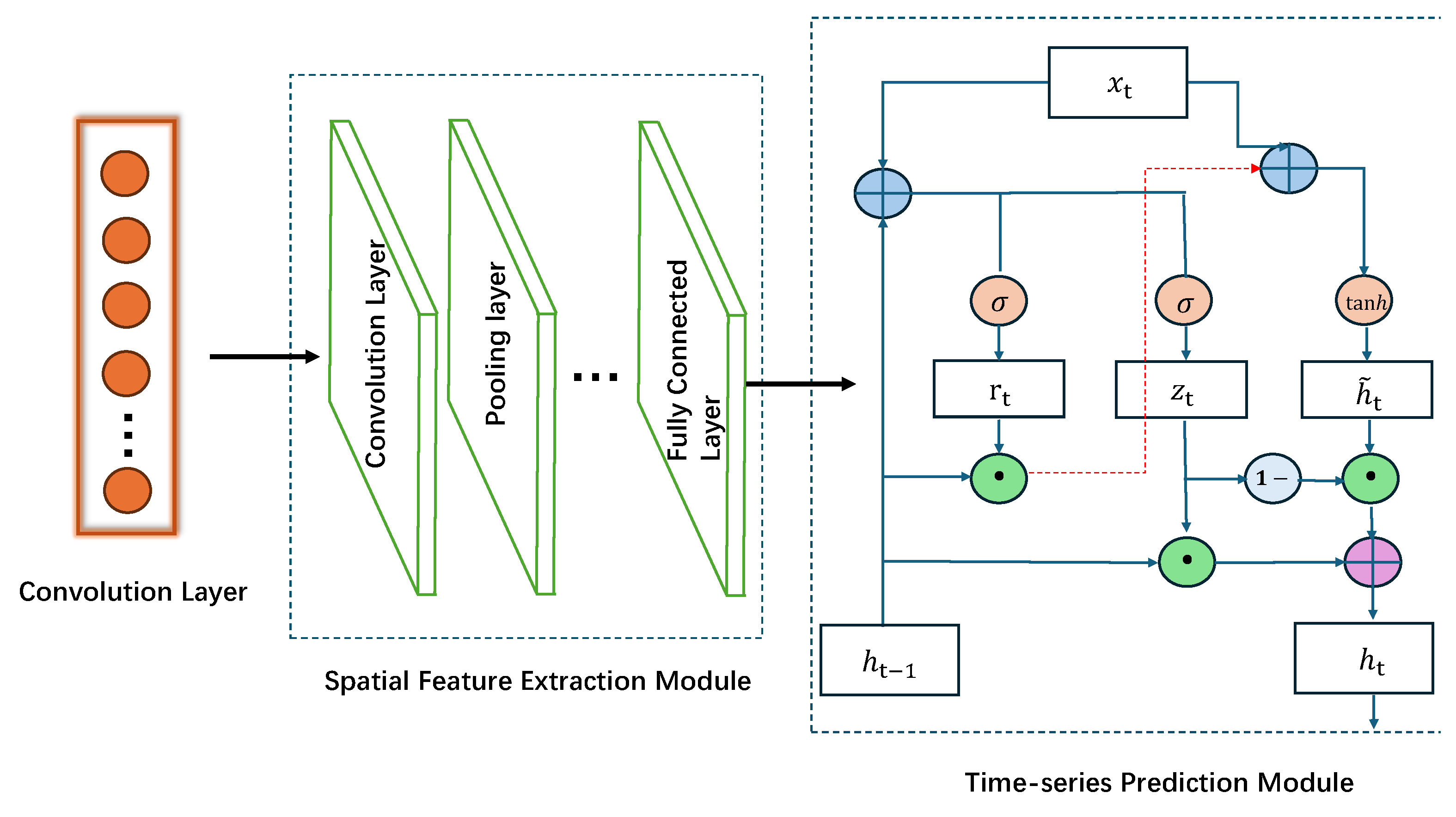
The CNN-GRU network architecture established in this research is composed of four principal modules: input sequence construction, local feature extraction via the Convolutional Neural Network (CNN), temporal dependency modeling using the Gated Recurrent Unit (GRU), and a final output fusion layer. A schematic representation of this framework is provided in Figure 1.

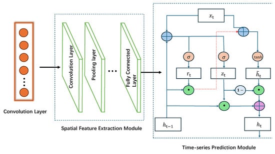
Figure 1. CNN-GRU Architecture Diagram.

2.2.1. Input Construction

For each modal component $u_k$ obtained from the VMD, a sliding window (with window length L and stride 1) is used for sampling to construct the input matrices:

$$X_k=\{x_{k,1},\dots ,x_{k,T}\}\in {\mathbb{R}}^{L\times T},X_{k,T}={[u_k\left(t\right),\dots ,u_k(t+L-1)]}^T.$$

(8)

Each $X_k$ is then fed into the network as time slices, which accommodates both the spatial patterns within a slice and the temporal evolution across slices.

2.2.2. CNN Local Feature Extraction

For each time slice $X_{k,t}\in {\mathbb{R}}^L$, a one-dimensional convolution and a max-pooling operation are performed to extract local spatial patterns [27]:

$$c_{k,t}^{\left(j\right)}=\mathrm{ReLU}(W_j\ast X_{k,t}+b_j)\in {\mathbb{R}}^{{\displaystyle \frac{L-f}{s}}+1},$$

(9)

where $W_j\in {\mathbb{R}}^f$ is the j-th convolutional kernel, s is the stride, and ∗ denotes the one-dimensional convolution. This is followed by a max_pooling operation:

$$p_{k,t}^{\left(j\right)}=\mathrm{max\_pooling}(c_{k,t}^{\left(j\right)}).$$

(10)

The outputs from the various convolutional kernels are then concatenated to form the multi-mode spatial feature vector for that time step:

$$f_{k,t}=\mathrm{concat}[p_{k,t}^{\left(1\right)};\dots ;p_{k,t}^{\left(J\right)}]\in {\mathbb{R}}^d.$$

2.2.3. GRU: Temporal Dependency Modeling

The feature sequence corresponding to each mode, denoted as ${\left\{f_{k,t}\right\}}_{t=1}^T$, is processed by a Gated Recurrent Unit (GRU) network employing a parameter-sharing mechanism. By governing the information dynamics through the update gate $z_t$ and the reset gate $r_t$, the GRU architecture effectively encodes long-range temporal correlations. The governing equations for the state updates are defined as:

$$\begin{array}{cc}\hfill z_t& =\sigma (W_z{f}_{k,t}+U_z{h}_{t-1}+b_z),\hfill \end{array}$$

(11)

$$\begin{array}{cc}\hfill r_t& =\sigma (W_r{f}_{k,t}+U_r{h}_{t-1}+b_r),\hfill \end{array}$$

(12)

$$\begin{array}{cc}\hfill {\tilde{h}}_t& =tanh(W{f}_{k,t}+U(r_t\odot h_{t-1})+b),\hfill \end{array}$$

(13)

$$\begin{array}{cc}\hfill h_t& =(1-z_t)\odot h_{t-1}+z_t\odot {\tilde{h}}_t,\hfill \end{array}$$

(14)

where $\sigma$ identifies the Sigmoid activation function, while the operator ⊙ denotes the element-wise multiplication. Consequently, the hidden state derived at the terminal time step, $h_t$, is adopted as the comprehensive feature representation for the entire input sequence.

2.2.4. Fusion and Output

The hidden states of the K modes at the final time step are concatenated:

$$\mathbf{H}=\mathrm{concat}[{\mathbf{h}}_{1,T};\dots ;{\mathbf{h}}_{K,T}]\in {\mathbb{R}}^{KH}.$$

(15)

The terminal hidden state yielded by the GRU at the final time increment, ${\mathbf{h}}_T$, is interpreted as the consolidated embedding $\mathbf{H}$, which encapsulates the spatio-temporal characteristics of the entire input series. This embedding vector is subsequently propagated through a fully connected layer to generate the final prediction, $\widehat{y}$, corresponding to the estimated crack width of the target sensor for the next time step:

$$\widehat{y}={\mathbf{W}}_{out}\mathbf{H}+{\mathbf{b}}_{out}.$$

(16)

3. The Proposed Imputation Method

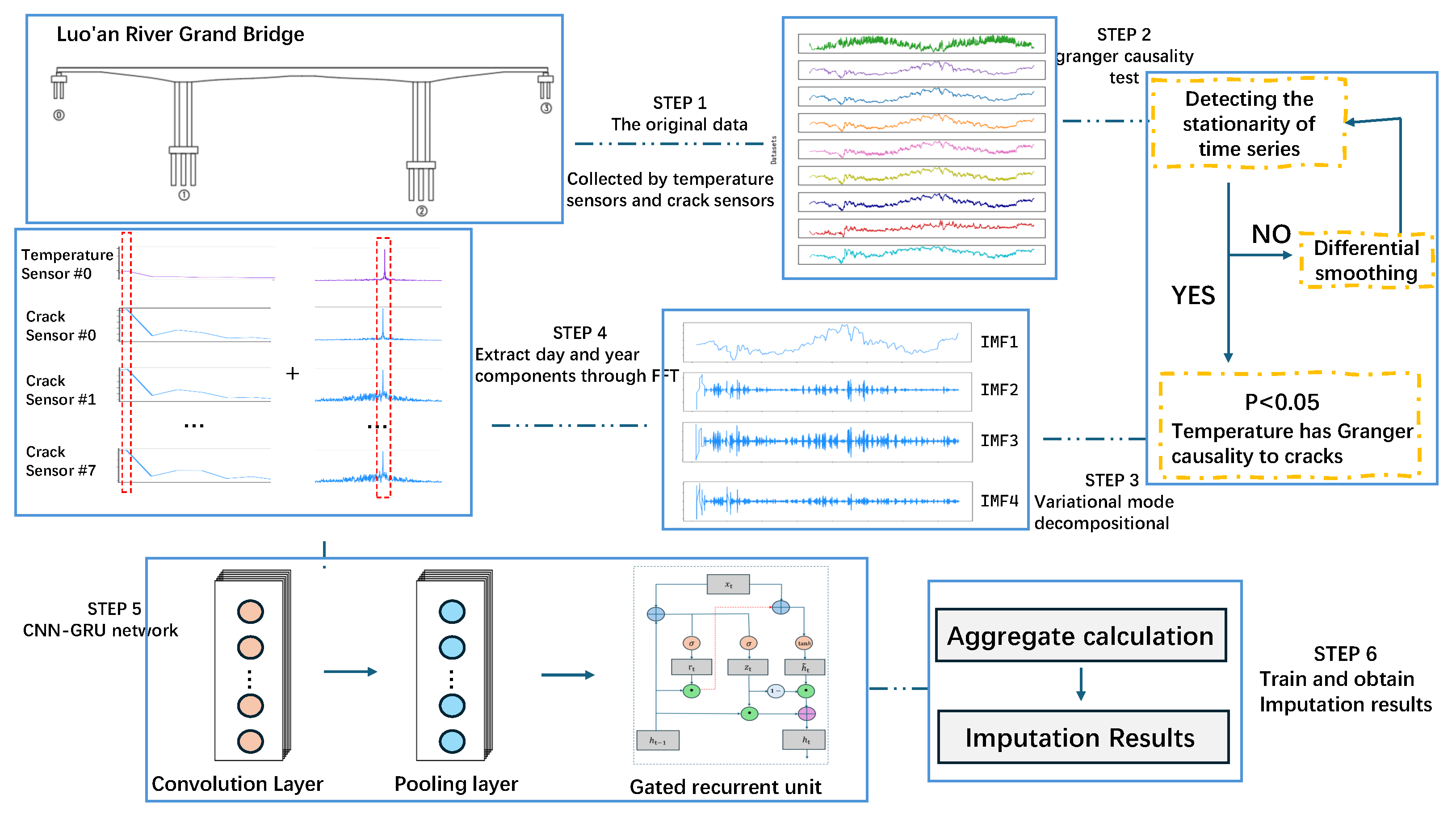
The core workflow of this framework comprises two main stages: data extraction and data imputation [28]. First, Shared-Period Variational Mode Decomposition (SP-VMD) is deployed to identify shared frequency components within the temperature and crack datasets, thereby isolating the authentic crack evolution trends driven by thermal factors. Subsequently, the extracted signal components are input into a CNN-GRU network for training, facilitating the reconstruction of missing crack observations. Finally, the imputation accuracy is assessed through a comprehensive set of performance metrics. The detailed procedural sequence is illustrated in Figure 2.

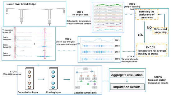
Figure 2. The procedures of the proposed SP-VMD-CNN-GRU model.

3.1. Validation of Temperature-Crack Causality

The fundamental prior knowledge underpinning this study is that environmental temperature variation is the primary external driver governing the opening and closing of bridge cracks. To rigorously validate this hypothesis, the Granger causality test is conducted before decomposition to quantify the predictive power of the temperature series regarding the crack width series.

The Granger causality test requires that the time series be stationary [29,30]. Therefore, the Augmented Dickey-Fuller (ADF) test is first employed to assess the stationarity of the original temperature and crack series [31]. The ADF test results (Table 1) indicate that both the original temperature and crack series exhibit non-stationary characteristics. However, following the application of first-order differencing, all series satisfied the stationarity test ($p<0.05$), thus fulfilling the prerequisite for executing the Granger causality test.

Table 1. ADF Test Results.

Time Series	Differential Order	T-Value	p-Value	Threshold			Test Results
				1%	5%	10%
temperature	0	−4.3785	0.000324	−3.4308	−2.8617	−2.5669	Stationary
crack#0	0	−2.0223	0.2769	−3.4308	−2.8617	−2.5669	non-Stationary
crack#0	1	−20.0723	0.0000	−3.4308	−2.8617	−2.5669	stationary
crack#1	0	−1.8775	0.3427	−3.4308	−2.8617	−2.5669	non-Stationary
crack#1	1	−14.4690	0.0000	−3.4308	−2.8617	−2.5669	stationary
crack#2	0	−1.8810	0.3411	−3.4308	−2.8617	−2.5669	non-Stationary
crack#2	1	−16.1830	0.0000	−3.4308	−2.8617	−2.5669	stationary
crack#3	0	−2.1091	0.2409	−3.4308	−2.8617	−2.5669	non-Stationary
crack#3	1	−20.2204	0.0000	−3.4308	−2.8617	−2.5669	stationary
crack#4	0	−2.1329	0.2315	−3.4308	−2.8617	−2.5669	non-Stationary
crack#4	1	−19.0036	0.0000	−3.4308	−2.8617	−2.5669	stationary
crack#5	0	−2.1251	0.2345	−3.4308	−2.8617	−2.5669	non-Stationary
crack#5	1	−19.5325	0.0000	−3.4308	−2.8617	−2.5669	stationary
crack#6	0	−3.5053	0.0079	−3.4308	−2.8617	−2.5669	Stationary
crack#7	0	−2.5397	0.1061	−3.4308	−2.8617	−2.5669	non-Stationary
crack#7	1	−19.8719	0.0000	−3.4308	−2.8617	−2.5669	stationary

On this basis, the Granger causality assessment is executed using the first-order differenced sequences, specifically investigating the directional causality defined as “temperature → crack”. A lag order of 24 is selected to comprehensively encompass the temporal dynamics of the diurnal cycle. The empirical results, detailed in Table 2, demonstrate that the F-statistics calculated for all eight monitoring channels significantly surpassed the requisite critical thresholds, yielding p-Values uniformly at 0.0000. Consequently, the null hypothesis—positing that temperature does not constitute a Granger cause of crack width fluctuations—is decisively rejected.

Table 2. Granger Causality Test Results.

Causality Direction	Lags	F-Value	p-Value	Causal Relationship Exists
Temperature → Crack#0	24	20.170998	0.000000	Reject
Temperature → Crack#1	24	21.394698	0.000000	Reject
Temperature → Crack#2	24	62.696268	0.000000	Reject
Temperature → Crack#3	24	115.460725	0.000000	Reject
Temperature → Crack#4	24	143.174625	0.000000	Reject
Temperature → Crack#5	24	124.081892	0.000000	Reject
Temperature → Crack#6	24	63.103818	0.000000	Reject
Temperature → Crack#7	24	45.726747	0.000000	Reject

This test result provides robust statistical evidence for the prior knowledge that “temperature change is a significant driving factor for crack width”, laying a solid theoretical foundation for the subsequent use of SP-VMD to isolate and extract the temperature-dominated crack evolution trend.

It is crucial to clarify that the Granger causality discussed herein primarily establishes a statistical predictive relationship rather than a comprehensive physical description. The rejection of the null hypothesis confirms that historical temperature data contains significant information for reducing the forecast error of crack width. While we recognize that bridge crack evolution is a complex process influenced by multiple coupled factors—including stochastic traffic loading and long-term material creep—this bivariate test is specifically designed to validate the predictive relevance of the thermal component. Given that the lag order ($p=24$) matches the diurnal cycle, the test results provide robust justification for treating temperature as a dominant quasi-periodic driver in this context, even though other latent physical variables are not explicitly parameterized in this specific step.

3.2. Procedure of the Proposed Method

The workflow of the method proposed in this paper is illustrated in Figure 2, and the specific implementation proceeds through the following four steps. First, the crack data acquired by two crack sensors in the inner section of the mid-span box girder of the left span, two crack sensors in the inner section of the mid-span box girder of the right span, and four crack sensors in the inner section of the mid-span box girder of the center span, as well as the temperature data recorded by the ambient temperature sensor on the bridge deck at mid-span, are selected as the subjects of analysis. From left to right, the crack sensors are labeled as #0 to #7 in turn. Second, the Granger causality test is employed to strictly verify the statistical validity of the prior knowledge that temperature change is the main driving force of fracture evolution. Leveraging this validated premise, the proposed SP-VMD algorithm is applied to synchronize the annual and daily variation trends of temperature and crack series, thereby extracting the authentic deformation component dominated by temperature. Third, a dataset is constructed using the extracted crack trend data, partitioned with a training-to-testing ratio of 9:1. Finally, the crack trends from multiple functional sensors serve as model inputs, while the trend from the target (faulty) sensor serves as the output. The training results across varying channel configurations are evaluated using performance metrics to determine the optimal number of input channels and achieve effective imputation of the crack data.

3.3. Evaluation Metrics for Imputation Results

To comprehensively assess the model’s performance, Root Mean Square Error (RMSE), Mean Absolute Error (MAE), Mean Absolute Percentage Error (MAPE), and the Coefficient of Determination ($R^2$) are selected as evaluation metrics [32].

RMSE amplifies larger errors through its squaring operation, making it highly sensitive to significant deviations between predicted and actual values, and is thus suitable for scenarios where emphasizing extreme errors is important. MAE directly reflects the average absolute value of the prediction error and is not sensitive to outliers, providing a robust estimate of the error distribution. MAPE expresses the mean absolute deviation as a percentage, which facilitates comparisons across datasets of different scales, although its calculation requires that the actual values are non-zero. $R^2$ is used to quantify the extent to which the model explains the variability of the target variable; a value closer to 1 indicates a better model fit.

$$\mathrm{RMSE}=\sqrt{{\displaystyle \frac{1}{n}}\sum _{i=1}^n{(y_i-{\widehat{y}}_i)}^2},$$

(17)

$$\mathrm{MAPE}={\displaystyle \frac{100\%}{n}}\sum _{i=1}^n\left|{\displaystyle \frac{y_i-{\widehat{y}}_i}{y_i}}\right|,$$

(18)

$$\mathrm{MAE}={\displaystyle \frac{1}{n}}\sum _{i=1}^n|y_i-{\widehat{y}}_i|,$$

(19)

$$R^2=1-{\displaystyle \frac{{\sum }_{i=1}^n{(y_i-{\widehat{y}}_i)}^2}{{\sum }_{i=1}^n{(y_i-\overline{y})}^2}},$$

(20)

where n denotes the total number of crack data samples, $y_i$ represents the actual crack data value, ($y_i$) indicates the predicted crack data value, and $y_i$ signifies the actual average value of the crack data.

4. Case Study

4.1. Project Overview

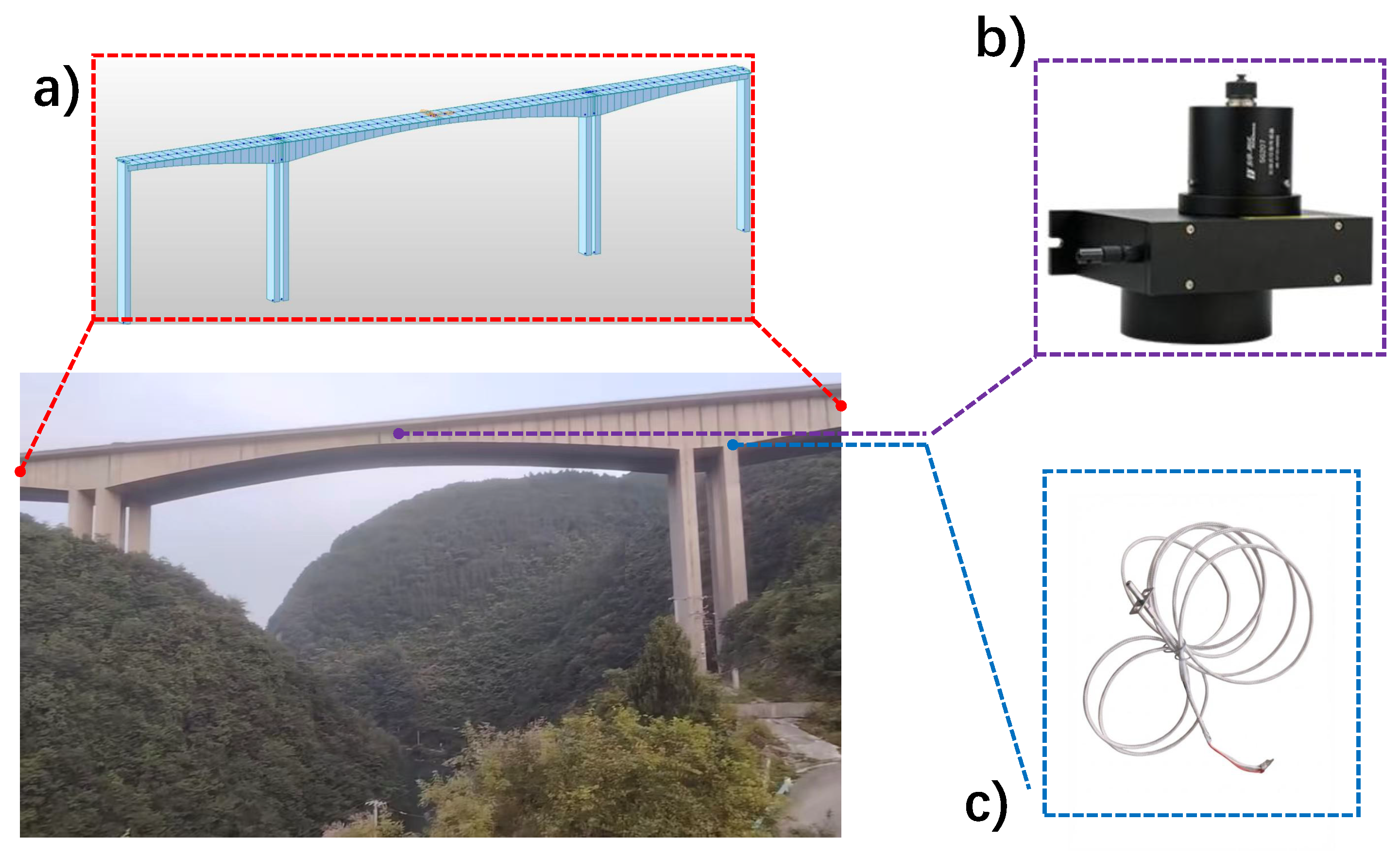
The engineering background for this study is the Luo’an River Grand Bridge. This bridge is situated on the G56 Hangzhou-Ruili Expressway (Zunyi section) and spans the Luo’an River, a third-level tributary of the Wu River in Zunyi County. The bridge site is connected to the G326 national highway via rural roads. The bridge site and the interior of the box girder are depicted in Figure 3. The bridge serves as the main line, with a central pile number of K1583+014 and a total length of 381 m. The superstructure is a (95 + 180 + 95) m variable cross-section, prestressed concrete continuous rigid frame. The box girder has a single-box, single-cell cross-section with straight webs; the top slab is 12.75 m wide, and the bottom slab is 7 m wide. The beam height of the box girder is 11.5 m at the root and 4.0 m at the mid-span and side-span closure sections. The lower edge of the bottom slab varies according to a 1.6-power parabola. The main piers of the down-line bridge are double hollow thin-walled piers, measuring 7 m in the transverse direction and 3 m in width, with a 13 m spacing between the outer edges of the double walls. The main pier foundation employs a monolithic cap, 5 m in thickness, supported by 18 bored piles, each with a diameter of 2.5 m. The piles are designed as end-bearing piles.

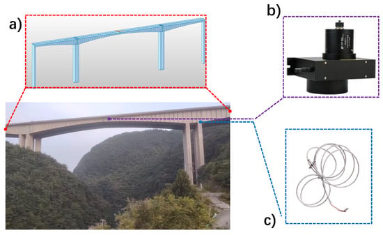
Figure 3. Overview of the Luo’an River Grand Bridge and its SHM system instrumentation: (a) Full view of the bridge and its Finite Element Model; (b) Schematic of the pull-wire displacement sensor for crack monitoring; (c) Diagram of the temperature sensor.

For structural analysis, a spatial frame model of the Luo’an River Grand Bridge is developed using the general-purpose finite element software MIDAS/Civil 2022. The superstructure is discretized using spatial beam elements, dividing the entire bridge into 92 elements and 97 nodes. The finite element model of the main bridge is shown in Figure 3a.

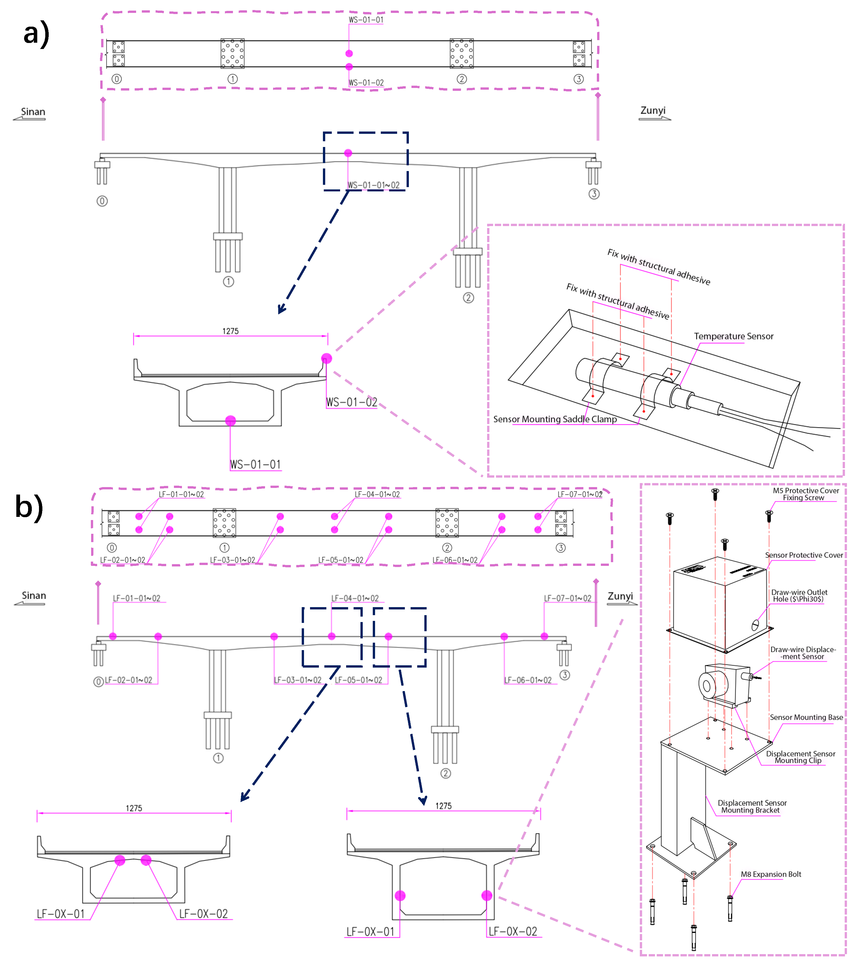
A Structural Health Monitoring (SHM) system is implemented on the Luoyang River Grand Bridge (Upstream line) to support structural assessment. The monitoring network consists of 14 crack meters (Model: MPS-XXS-100-R, Shenzhen Miran Technology Co., Ltd., Shenzhen, China; Range: 25 mm; Resolution: ≤0.01 mm) distributed across 7 sections to capture minute structural changes. As detailed in the sensor schematic in Figure 3b, these are pull-wire displacement sensors operating on a potentiometric principle, where the linear extension of the wire—driven by crack opening—is converted into precise voltage signals. Complementing this, two high-precision temperature sensors (Model: BD-SP-PT100, Sichuan Bodian Technology Co., Ltd., Chengdu, China; Accuracy: ≤0.5 °C) are installed to track thermal conditions. As depicted in Figure 3c, the temperature sensors are firmly anchored using structural adhesive and saddle clamps adjacent to the crack meters, ensuring strict spatial synchronization between thermodynamic and mechanical data. To collect the diurnal and annual datasets required for this study, the system utilizes an automated data acquisition pipeline. Analog signals are digitized by a local DAQ unit at a sampling frequency of 1 Hz and transmitted wirelessly via a 4G network to a cloud server, ensuring continuous, gap-free time-series recording without manual intervention. The spatial layout and technical details of the instruments are illustrated in Figure 4. Specifically, Figure 4a depicts the temperature sensor, while Figure 4b shows the crack sensor.

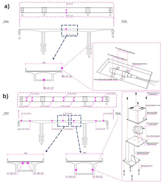
Figure 4. Schematic layout and instrumentation details of the monitoring system: (a) Temperature sensors; (b) Crack sensors.

4.2. Data Preprocessing

The dataset is derived from actual records collected by the field monitoring system of the Luo’an River Grand Bridge, representing structural response data under real-world environmental conditions. Due to factors such as on-site environmental interference, fluctuations in sensor performance, and instability in the transmission link, the sampling intervals of the raw data exhibit a certain degree of variation. To eliminate the impact of irregular sampling on time-series analysis, the raw data is resampled to a uniform interval of 1 h [33]. Specifically, the arithmetic mean of all sample points within each hour is taken as the representative value for that time segment, thereby forming an evenly spaced time series. For anomalous values (outliers) present in the dataset, such as those significantly deviating from the normal range due to transient interference or temporary equipment faults, a linear interpolation method within the temporal neighborhood is used for correction. This involves replacing the outlier with the average of the valid observations from the immediately adjacent time periods (one sampling period before and one after). This approach effectively smooths out atypical transient disturbances while preserving the overall trend of the data, thereby enhancing the consistency and quality of the dataset and providing a more reliable foundation for subsequent modeling and analysis.

To ensure numerical stability and fair comparison across different models, all resampled time series are normalized to the range of $[0,1]$ using Min-Max scaling, defined as:

$$x_{norm}={\displaystyle \frac{x-x_{min}}{x_{max}-x_{min}}},$$

(21)

where $x_{min}$ and $x_{max}$ are the minimum and maximum values of the training dataset, respectively. It should be noted that the validation and testing sets are scaled using the same parameters derived from the training set to prevent data leakage. All error metrics, including RMSE and MAE, are calculated based on the original physical scale of the crack width (mm) to ensure that the reported predictive accuracy reflects actual engineering requirements.

4.3. Time Step of Input Variables

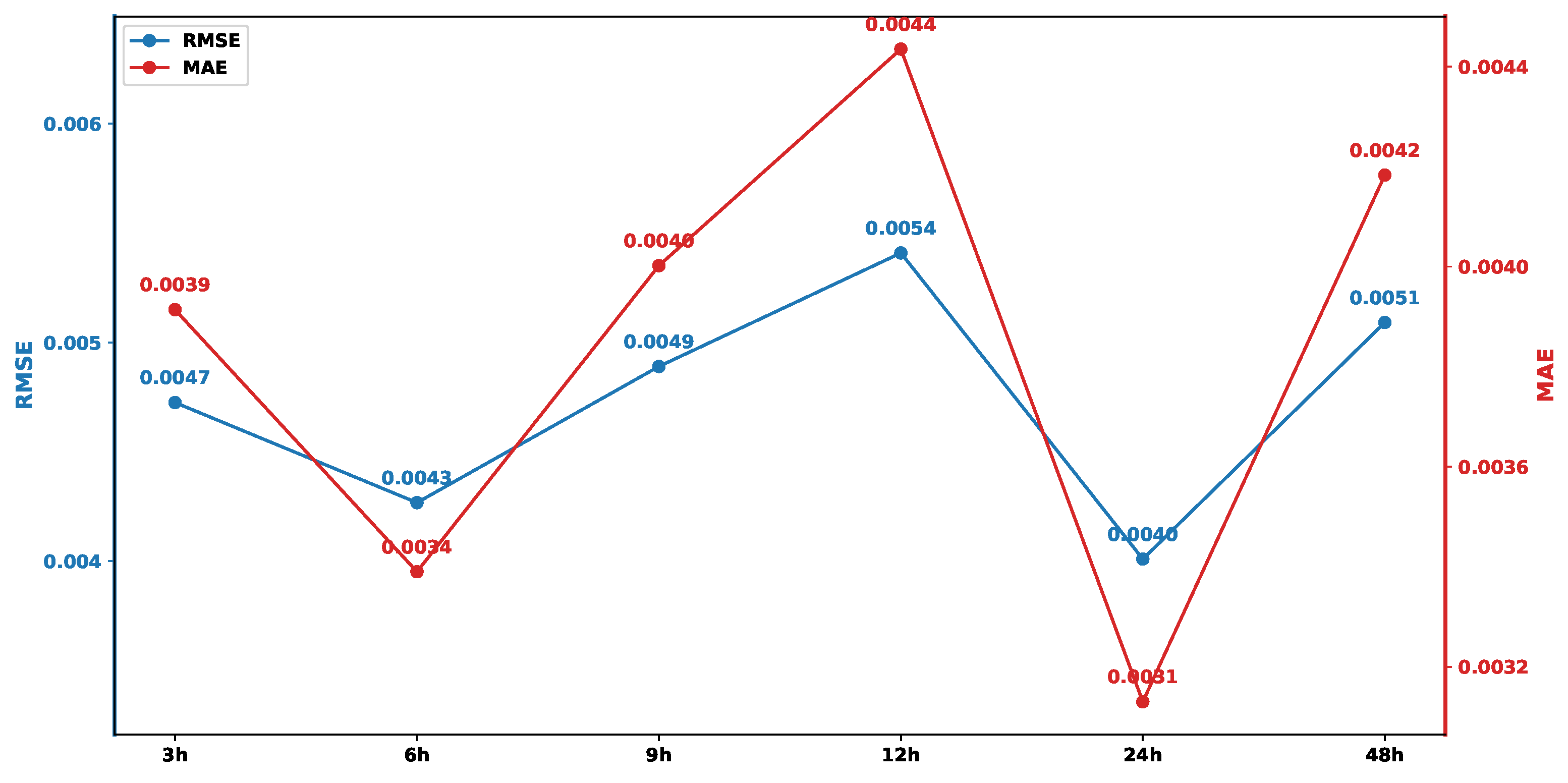
To determine the optimal historical time step for the model input, the effects of six different settings—3 h, 6 h, 9 h, 12 h, 24 h, and 48 h—on prediction performance are comparatively analyzed. An excessively short historical time step may limit the model’s ability to fully learn the temporal features, whereas an overly long one can easily introduce noise, leading to overfitting [34]. As shown in Figure 5, the Root Mean Square Error (RMSE) and Mean Absolute Error (MAE) of the model exhibit a distinct trend under different time steps. When the time step is set to 24 h, both the RMSE and MAE reached their minimum values (0.0031 and 0.0040, respectively), indicating that the model achieved its optimal prediction accuracy and stability at this point. Therefore, the historical time step for the input variables is determined to be 24 h. It is important to clarify that while a 24-h window primarily targets the capture of short-term diurnal loop characteristics, the seasonal thermodynamic context is not lost. Since the input data is the reconstructed signal incorporating the annual trend component (IMF1) extracted via SP-VMD, the seasonal “thermal boundaries” (e.g., the expansion in summer or contraction in winter) are inherently encoded in the varying baseline amplitude of the time series. Consequently, the model can perceive the macro-seasonal state through the magnitude of the data within the 24-h window, without requiring an excessively long input sequence (e.g., 365 days) to learn the annual context.

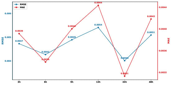
Figure 5. Testing errors using different time steps.

4.4. Number of Modes for VMD

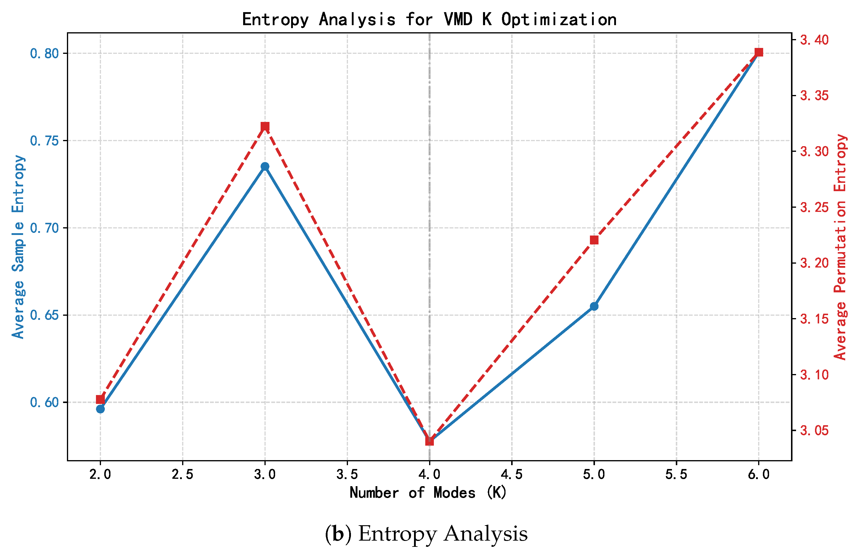
The performance of VMD relies on selecting an appropriate number of modes (K) to balance signal separation fidelity against the risk of over-decomposition. Instead of relying on arbitrary empirical selection, we determine the optimal K through a rigorous dual-validation strategy combining physical consistency (Center Frequency Method) and statistical complexity (Entropy Analysis), as illustrated in Figure 6.

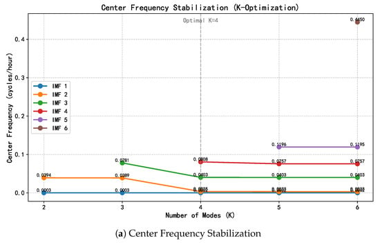
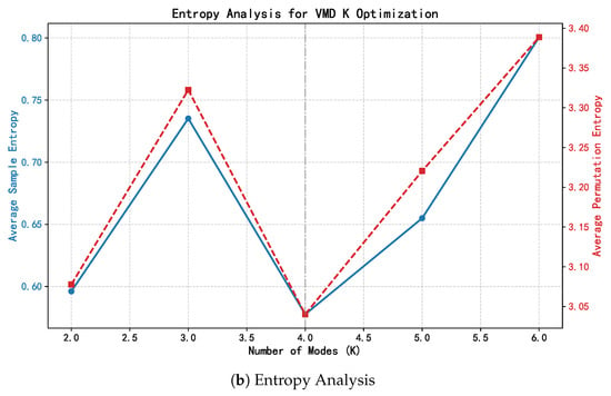
Figure 6. Dual-validation for optimal K selection: (a) Center Frequency Stabilization, illustrating the convergence of physical modes (IMF 1 and IMF 3) at $K=4$ without spectral aliasing; (b) Entropy Analysis, indicating a global minimum in sample entropy at $K=4$, which confirms the most orderly decomposition.

Figure 6a depicts the application of the Center Frequency Stabilization Criterion. Observing the spectral evolution for $K\in [2,6]$, the dominant thermodynamic components—specifically the annual trend (IMF 1, ≈0.0002 cph) and the diurnal cycle (IMF 3, ≈0.040 cph)—exhibit distinct convergence at $K=4$. Crucially, the spectral intervals between these modes remain distinct, providing clear evidence that no mode aliasing or adjacency occurs at this decomposition level. When K is increased to 5, the primary physical modes remain stable, whereas the newly emerged component (≈0.12 cph) manifests as high-frequency stochastic noise rather than a structural response.

Complementing this spectral analysis, the Entropy Analysis presented in Figure 6b offers a quantitative validation. The evolution of Sample Entropy (SampEn) reveals a characteristic “V-shaped” trajectory: a sharp spike at $K=3$ indicates severe mode mixing where multiple physical scales are entangled, followed by a drastic reduction to a global minimum at $K=4$ (SampEn $\approx 0.58$). This minimum signifies that the signal has been optimally decoupled into orderly, deterministic physical trends. Conversely, the subsequent entropy rise at $K>4$ reflects the intrusion of high-entropy noise. Collectively, these physical and statistical metrics robustly identify $K=4$ as the optimal parameter.

4.5. Crack Data Extraction

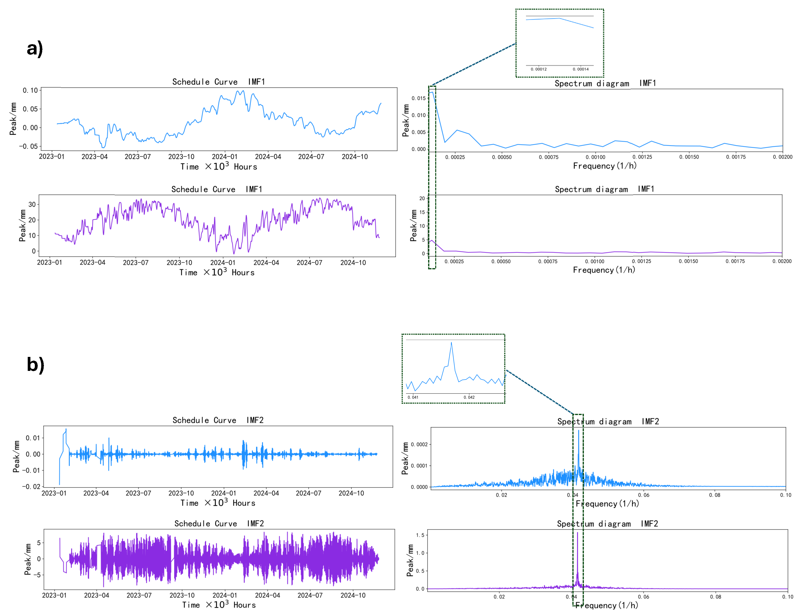
After determining the optimal number of modes, Variational Mode Decomposition is performed on the temperature data and the crack data, respectively. Taking the crack data collected by sensor #0 as an example, its VMD decomposition results are shown in Figure 7. By applying a Fast Fourier Transform to each Intrinsic Mode Function (IMF), the frequency spectra distributions for the temperature and crack signals are obtained. The spectrum analysis revealed that the IMF1 components of both the temperature and crack data exhibit a significant peak at a frequency of 0.000114. Given that the data sampling interval is 1 h, with a total of 24 sample points per day, the period corresponding to this frequency is: $1/(0.000114\times 24)=365.5$ days [35]. This period is approximately one year, indicating that IMF1 effectively reflects the annual cycle characteristics, which can be attributed to the influence of seasonal temperature variations on the structure. On the other hand, the IMF2 component shows a peak at a frequency of 0.041683, with a corresponding period of: $1/(0.041683\times 24)=1.0$ day. This indicates that IMF2 captures the periodic fluctuations on a daily basis, primarily reflecting the structural response caused by diurnal temperature differences. Based on these shared-period features, the annual-cycle IMF and the diurnal-cycle IMF, which are common to both the temperature and crack data, are extracted. Although a degree of spectral overlap may exist between seasonal thermal effects and early-stage shrinkage, the dominant power of the annual cycle allows IMF1 to serve as a high-fidelity proxy for the temperature-induced response. By reconstructing these shared-period components, the model establishes a physically consistent input, effectively mitigating the interference of non-thermal stochastic noise.

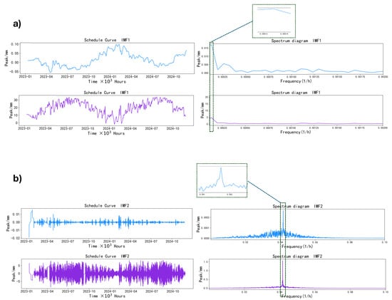
Figure 7. #0 Crack Data Decomposition Results (a,b).

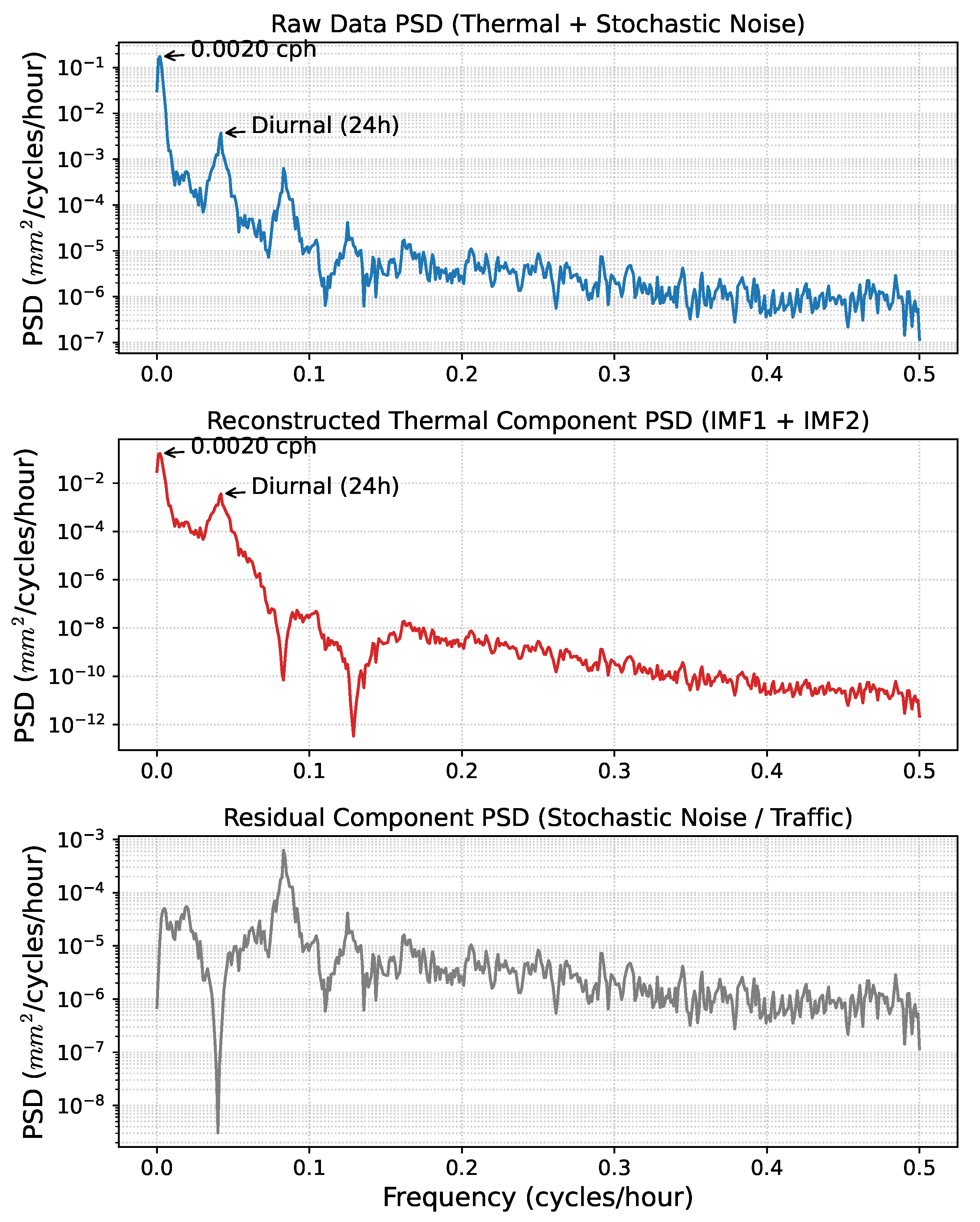
To rigorously validate the efficacy of the proposed decomposition strategy, a comparative Power Spectral Density (PSD) analysis is performed on the raw monitoring data, the extracted thermal component, and the residual component, as illustrated in Figure 8. As observed in the middle panel, the reconstructed signal (comprising IMF1 and IMF2) strictly preserves the deterministic Annual (0.0020 cph) and Diurnal (0.0417 cph) spectral peaks. Crucially, these peaks manifest as sharp, narrowband features, demonstrating the retention of smooth thermodynamic responses while suppressing the background noise floor by several orders of magnitude. In sharp contrast, the residual component (bottom panel) effectively isolates non-thermal disturbances, which appear as broadband stochastic fluctuations ($0.1–0.5$ cph) typical of dynamic vehicle loads and measurement noise. Most notably, the semi-diurnal component (≈0.08 cph)—often exhibiting spectral overlap between secondary thermal harmonics and the dual-peak patterns of traffic rush hours—is conservatively retained in the residual to ensure the physical purity of the input baseline. This distinct spectral separation quantitatively confirms that the SP-VMD framework functions as a physics-guided narrowband filter, successfully decoupling the dominant, physics-governed structural response from broadband stochastic interference.

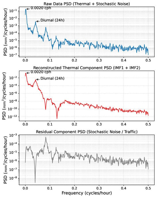
Figure 8. Power Spectral Density (PSD) comparison of the raw, reconstructed, and residual signals validating the effective isolation of thermal trends from stochastic noise.

4.6. Data Management and Spatial Correlation Analysis

To guarantee the reproducibility and physical fidelity of our data-driven framework, a rigorous management protocol is established. This study utilizes an extensive longitudinal dataset spanning 12 January 2023, to 25 November 2024 ($N\approx \mathrm{15,402}$ hourly samples). Unlike short-term records, this period encompasses nearly two complete annual cycles, capturing the full spectrum of seasonal thermodynamic variations. Prior to model ingestion, raw signals are refined via the SP-VMD method. By isolating deterministic annual and diurnal components, this physics-guided filtering process effectively decouples the temperature-driven structural response from high-frequency stochastic noise, yielding robust “Temperature-Crack” pairs.

Feature selection is governed by spatial correlation analysis to exploit the collaborative sensing potential of the network. Designating the mid-span sensor (#2) as the target faulty node, we quantified its linear dependence with neighboring channels (Table 3). A distinct spatial decay law emerged: sensors within the same cross-section exhibited near-unity correlation, followed closely by those in the adjacent left span (>0.98), whereas distal sensors in the right span showed the weakest linkage. This decay characteristic provides a solid physical basis for prioritizing highly correlated neighbors to reconstruct the target signal.

Table 3. Correlation Coefficients Between Different Sensors and #2.

Rank	1	2	3	4	5	6	7	8
Sensor number	#2	#5	#4	#0	#1	#3	#7	#6
Correlation coefficient with # 2	1	0.99200	0.98868	0.98658	0.98124	0.96563	0.86483	0.54293

Data partitioning adhered to a strict chronological protocol to eliminate temporal data leakage. The dataset is divided into a Training Set (first 90%) and a Testing Set (final 10%). While validation splits are customary for mitigating overfitting in limited datasets, the extensive temporal horizon of this study offers a superior safeguard. By enabling the model to learn comprehensive seasonal dynamics—such as summer expansion and winter contraction—over multiple years, combined with Dropout regularization (0.5), we ensure robust generalization without the need to sequester data for a separate validation split.

4.7. Structure of the CNN-GRU Model

A multi-layer CNN-GRU network can more effectively extract and characterize the complex features within the data, thereby enhancing prediction performance. However, excessive structural complexity must be avoided to mitigate the risk of overfitting [36]. Therefore, the appropriate setting of the model’s architecture and hyperparameters is particularly crucial.

To validate the model’s effectiveness, multiple iterative experiments are conducted. The results indicate that the CNN-GRU model can effectively capture the dynamic trends of the crack data. As shown by the evaluation metrics listed in Table 4, the Coefficient of Determination ($R^2$) in all test scenarios is higher than 0.9500, which demonstrates a high degree of consistency between the predicted and measured values at each layer and signifies a good model fit. Further architectural comparisons revealed that a network comprising one CNN layer and two GRU layers performed optimally. Its prediction curve most closely matched the actual observed values, suggesting that a moderate level of complexity is beneficial for balancing the model’s expressive power and generalization performance. After extensive hyperparameter optimization, the final model hyperparameters are determined as follows: Given the multivariate 1D time-series nature of the bridge crack data, a 1D Convolutional Neural Network (1D-CNN) is employed to extract local feature patterns. Specifically, the CNN layer is configured with 256 filters, a kernel size of 2, a stride of 1, and a padding of 2. The extracted features are then processed by a Max-Pooling layer before being fed into a 2-layer GRU with a hidden size of 64 and a dropout ratio of 0.5. The Adam optimizer is selected with a learning rate of 0.00001, a batch size of 64, and a training duration of 100 epochs. The Mean Squared Error (MSE) is employed as the loss function to optimize the accuracy of the regression prediction

Table 4. Comparison of Metrics Across Different Models.

Network Layer	RMSE	MAE	MAPE	${\mathit{R}}^2$
2 × GRU–1 × CNN	0.00401	0.00313	12.94702	0.99160
3 × GRU–2 × CNN	0.00458	0.00366	17.10346	0.98904
4 × GRU–3 × CNN	0.00504	0.00398	24.95129	0.98671
5 × GRU–4 × CNN	0.00688	0.00575	32.38042	0.97530

4.8. Model Training

The specific configuration for this training is detailed in Table 5. The training strategy is structured to progressively evaluate the efficacy of spatial information through a hierarchical experimental design. We initiate the process with a single-channel baseline, where the model is tasked with reconstructing the trajectory of the target sensor (#2), relying exclusively on the input from sensor #5. To capture more complex local dependencies, we advance to a dual-channel configuration by integrating data from sensor #4, effectively testing the model’s ability to synthesize information from adjacent monitoring points. The experiment culminated in a comprehensive multi-channel extension, where the input dimension is scaled to seven distinct channels—specifically comprising sensors #5, #4, #0, #1, #3, #7, and #6. This full-spectrum setup allows the model to leverage global spatial correlations across the bridge span. Throughout these experimental phases, we adhere to a rigorous temporal partitioning protocol: the initial 90% of the sequential data is dedicated to optimizing the model parameters, while the final 10% is strictly reserved for validation purposes to monitor generalization performance and prevent overfitting.

Table 5. Comparison of Metrics Across Different Channel Counts.

Input Channels	RMSE	MAE	MAPE	R2
1-channel (#5)	0.01537	0.01402	60.11760	0.87651
2-channels (#5, #4)	0.01359	0.01200	47.82912	0.90349
3-channels (#5, #4, #0)	0.00686	0.00574	36.45446	0.97544
4-channels (#5, #4, #0, #1)	0.00470	0.00362	21.36438	0.98846
5-channels (#5, #4, #0, #1, #3)	0.00450	0.00354	18.54939	0.98940
6-channels (#5, #4, #0, #1, #3, #7)	0.00541	0.00442	24.01208	0.98470
7-channels (#5, #4, #0, #1, #3, #7, #6)	0.00401	0.00313	12.94702	0.99160

To guarantee the reproducibility of the experimental results, strict data processing protocols are implemented before the training loop. Firstly, the raw dataset underwent a cleaning procedure followed by global normalization to the [0,1] range. Subsequently, the SP-VMD mechanism is applied to each sensor channel using a penalty factor $\alpha =2000$ and $K=4$ modes. By performing FFT peak detection on the decomposed modes, we isolate and reconstruct the physics-guided trends—specifically the annual and diurnal components—which serve as the clean input for the model. These processed trends are then organized into input tensors using a sliding window of 24 h (stride=1) to preserve temporal continuity.

Regarding model configuration, the hyperparameter selection is driven by a rigorous sensitivity analysis rather than arbitrary assignment. We conduct a grid search across a range of learning rates $\{{10}^{-3},{10}^{-4},{10}^{-5}\}$ and batch sizes $\{32,64,128\}$ to identify the optimal convergence behavior. The analysis reveals that a learning rate of $1\times {10}^{-5}$ combined with a batch size of 64 provides the most stable gradient descent and the lowest validation loss. Consequently, the final CNN-GRU network is trained using these optimal parameters, employing the Adam optimizer and a Mean Squared Error (MSE) loss function over a course of 100 epochs. All experiments are executed using the PyTorch(version 2.7.1+cu126) framework on a computational platform equipped with an Intel i7-14650HX CPU(Intel Corporation, Santa Clara, CA, USA) and an NVIDIA RTX 4060 GPU (NVIDIA Corporation, Santa Clara, CA, USA). The computing platform is a Yaoshi 15 Pro laptop (MECHREVO, Beijing, China).

5. Results and Discussion

5.1. Imputation Results and Evaluation

Before evaluating the specific model architectures, we investigate the impact of spatial information density on imputation performance. As demonstrated in Table 6, imputation accuracy proves to be highly sensitive to the number of input sensor channels. Specifically, increasing the input from a single channel (#5) to five channels significantly reduces the RMSE from 0.01537 to 0.00450. This improvement confirms the hypothesis that a dense sensor array captures redundant spatial information effectively, which is critical for reconstructing missing signals. Notably, introducing the sixth channel resulted in a slight degradation in performance, with MAPE rising to 24.01%. This phenomenon suggests that incorporating sensors with weaker correlations—as identified in the previous correlation analysis—may introduce more noise than valid signal information. However, when the full set of seven channels is utilized, the model effectively learns to filter this noise, achieving an optimal RMSE of 0.00401. Consequently, the 7-channel configuration is established as the standard input for all subsequent comparative analyses.

Table 6. Comparison of Model Metrics.

Model Comparison	Training Time (s)	RMSE	MAE	MAPE	${\mathit{R}}^2$
TCN	1239.8	0.00002	0.00382	11.24866	0.98856
TCN_CNN	1233.1	0.00682	0.00561	34.97901	0.97570
LSTM	81.4	0.00687	0.00602	22.93783	0.97535
CNN_LSTM	87.7	0.00512	0.00406	18.07160	0.98631
GRU	85.7	0.00505	0.00394	23.52275	0.98670
CNN_GRU(w/o SP-VMD)	71.8	0.00690	0.00589	18.58792	0.97513
CNN_GRU(Proposed)	92.0	0.00401	0.00313	12.94702	0.99160

Note: Bold values indicate the best performance for each metric.

To validate the superiority of the proposed framework, we conduct a comparative analysis against five benchmark models, including TCN, LSTM, GRU, and their CNN-hybrid counterparts. To guarantee the fairness of this comparative analysis, we establish a strictly controlled experimental environment where all models are evaluated under identical conditions. Crucially, every candidate model receives the identical set of SP-VMD extracted features rather than raw noisy data, ensuring that any performance deviation is solely attributed to the neural network architecture’s ability to interpret these physics-guided trends. Furthermore, we standardize the hyperparameter configuration across all baselines—adopting the same 24-h look-back window, a unified 9:1 data partition, and the optimal learning rate and batch size identified in our sensitivity analysis. By aligning these preprocessing and training protocols, we successfully isolate the architectural efficiency of the models, confirming that the performance gains of the CNN-GRU derive from its superior spatio-temporal modeling capabilities rather than discrepancies in hyperparameter optimization or input quality.

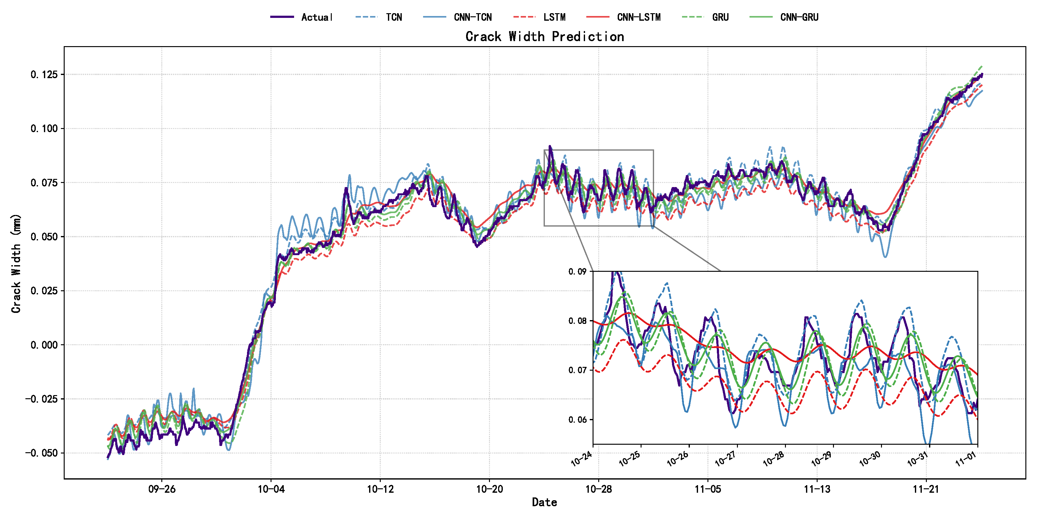
The comparative analysis, as visualized in Figure 9 and detailed in Table 7, indicates a discernible performance hierarchy wherein CNN-hybrid models consistently outperform their standalone counterparts, validating the synergy between local spatial feature extraction and temporal modeling. Among the evaluated architectures, the proposed CNN-GRU framework demonstrates superior predictive fidelity, yielding an $R^2$ of 0.9916 and a MAPE of 12.95%. To provide a comprehensive interpretation of these metrics—particularly the contrast between the near-perfect correlation and the percentage error—it is essential to interpret them within the physical characteristics of the target signal. The high $R^2$ value is grounded in the rigorous experimental design defined in Section 4.6, where a strict chronological split is implemented to reserve testing data, thereby mitigating temporal data leakage; rather than implying overfitting, this accuracy underscores the effectiveness of the physics-guided preprocessing, as the model focuses on recovering deterministic thermal trends (IMF1 + IMF2) isolated from high-frequency stochastic noise via SP-VMD. Conversely, the relatively high MAPE (>10%) is primarily influenced by the “small denominator effect” characteristic of micro-scale monitoring, where minute crack widths (approaching 0 mm) mathematically amplify marginal absolute deviations, rendering absolute error metrics (RMSE, MAE) and trend correlation ($R^2$) the more robust indicators of reconstruction fidelity in this engineering context.

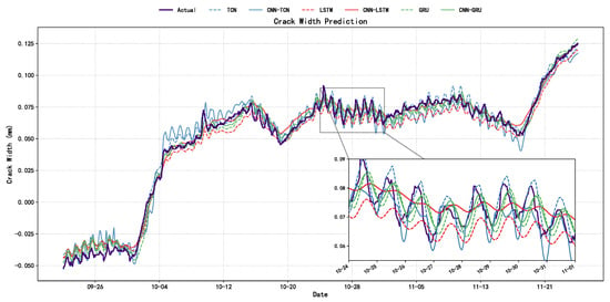
Figure 9. Comparison of Crack Data Imputation Using RNN, LSTM, and TCN Combined with CNN.

Table 7. Comparison of Validation Metrics Across Models.

Model Comparison	RMSE	MAE	MAPE	${\mathit{R}}^2$
TCN	0.01217	0.01039	17.84195	0.84501
TCN_CNN	0.03081	0.02476	57.52079	0.00719
LSTM	0.01074	0.00938	18.69620	0.87940
CNN_LSTM	0.00827	0.00670	20.10607	0.92852
GRU	0.00962	0.00825	19.49930	0.90320
CNN_GRU	0.00789	0.00670	18.84175	0.93494

Note: Bold values indicate the best performance for each metric.

While the SP-VMD framework effectively extracts temperature-driven periodicities, the inherent spectral overlap between thermal responses and long-term structural phenomena (e.g., creep or shrinkage) remains a subtle challenge. In this study, such non-periodic variations are treated as secondary to dominant thermal drivers. However, the precision of this physical decoupling is intrinsically tied to the fidelity of the monitoring data.

Consequently, the model’s performance relies on a substantial volume of high-quality monitoring records, as the presence of noise or outliers can impact the reconstruction accuracy. In practical SHM deployment, significant shifts in the monitoring environment, loading conditions, or structural state may alter the learned mapping between physical features and crack evolution. Under such circumstances, periodic data re-collection and model retraining would be necessary to maintain imputation fidelity, representing a requisite investment in computational resources and time.

5.2. Practicality Analysis

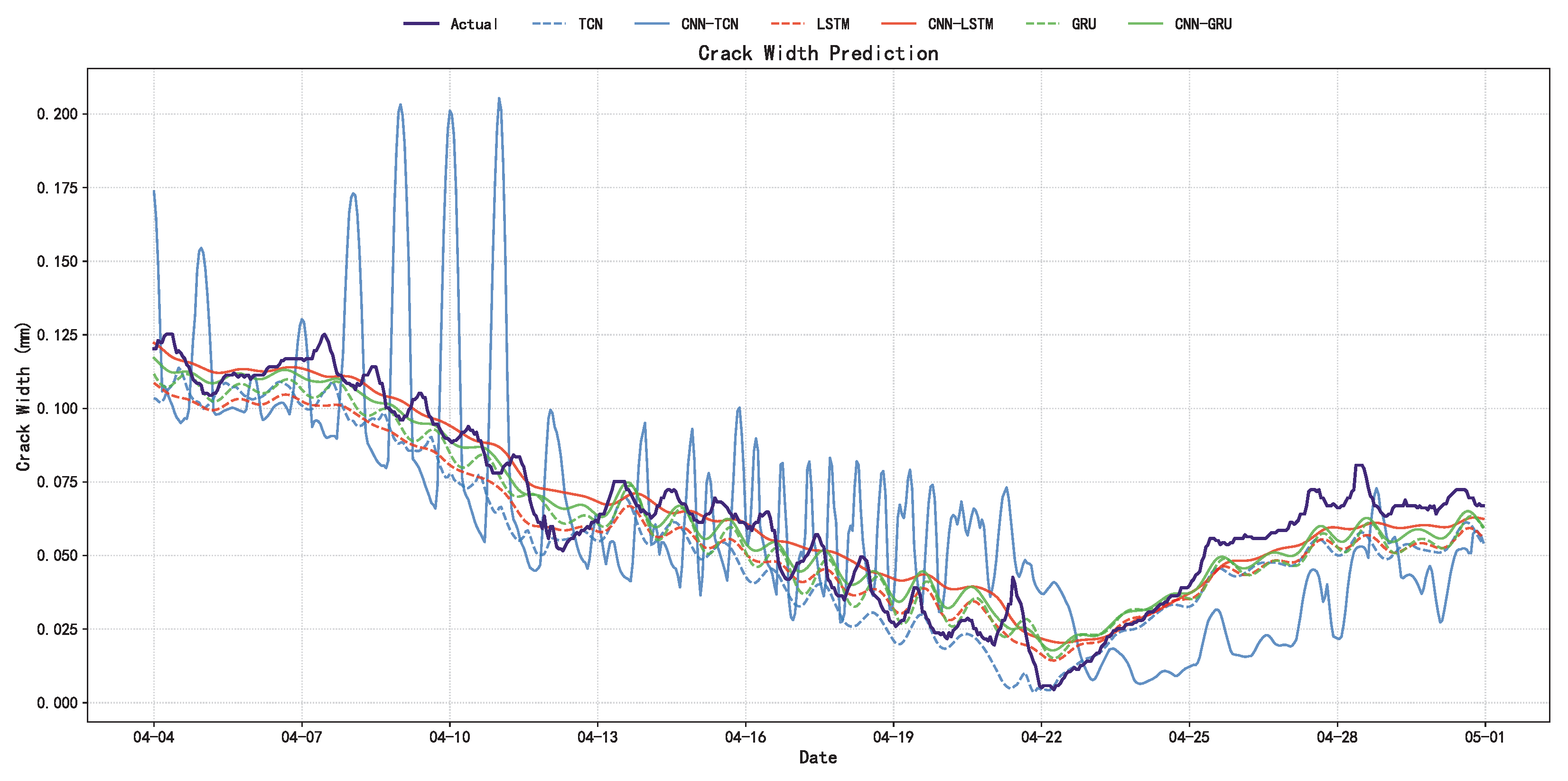
A robust Structural Health Monitoring (SHM) model must perform consistently across diverse time periods and environmental conditions. To evaluate this generalization capability, we apply the trained models to a new dataset recorded in spring (7 April to 2 May 2023), a period characterized by different thermal gradients compared to the autumn training set. The results, visualized in Figure 10 and detailed in Table 8, reinforce the findings from the primary experiment, showing that the CNN-GRU model maintains its performance lead with an $R^2$ of 0.9349 and an RMSE of 0.0079. Regarding dynamic response, significant differences emerge during the sharp fluctuations observed between 17 April and 22 April. While TCN-based models struggle to converge and exhibit large deviations, the CNN-GRU and CNN-LSTM models successfully capture the trend reversals. This stability is largely attributed to the SP-VMD preprocessing, which ensures that the input data retains clear, physically driven trends—specifically annual and diurnal components—enabling the deep learning model to generalize effectively even when the raw data distribution shifts due to seasonal changes.

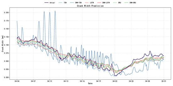
Figure 10. Comparison of imputation results for unseen data from a new annual cycle to evaluate the long-term robustness of the proposed model.

Table 8. Diebold–Mariano (DM) test statistics comparing the predictive accuracy of the proposed CNN-GRU against baseline models.

Model Comparison	DM Value
TCN	−9.028819
CNN_TCN	−20.064663
LSTM	−26.942710
CNN_LSTM	−16.911945
GRU	−13.857066
CNN_GRU	—

From the quantitative metrics in Table 8, the CNN-GRU model achieves the lowest RMSE (0.007887) and MAE (0.006701), alongside the highest $R^2$ (0.934941) among all comparators, signifying the smallest prediction error and the best goodness-of-fit. Although the CNN-LSTM performs closely in terms of the MAE metric, the CNN-GRU maintains a distinctive lead in both RMSE and $R^2$, demonstrating superior overall stability and explanatory power. In summary, the CNN-GRU model proves capable of accurately simulating the actual temporal evolution of cracks, establishing itself as the optimal choice in terms of both imputation accuracy and practical utility.

Beyond demonstrating temporal adaptability, the framework possesses broad potential for structural generalization by being anchored in fundamental physical principles. Although this study validated the method on a concrete bridge, the core mechanism—decoupling shared thermal drivers via SP-VMD—is theoretically transferable to other material types, including steel bridges. In fact, the distinct material properties of steel may further enhance the applicability of this approach. Since steel structures exhibit higher thermal conductivity and more pronounced thermal expansion than concrete, the thermally induced response is typically more significant relative to background noise. This higher signal-to-noise ratio (SNR) of the thermal component could theoretically facilitate the SP-VMD algorithm in identifying and extracting periodic trends. Given that the strategy fundamentally relies on frequency synchronization (periodicity) rather than absolute signal amplitude, the framework is expected to remain robust—and potentially more effective—when applied to steel infrastructure.

5.3. Statistical Tests

Before evaluating the comparative predictive performance, it is requisite to reaffirm the statistical validity of the temperature-driven mechanism that underpins the SP-VMD framework. Recalling the Granger Causality analysis presented in Section 3.1 (Table 2), the test results at a lag length of 24 h yielded F-statistics significantly surpassing the critical threshold, with p-values consistently at 0.0000 (≪0.05) across all sensor channels. This statistical evidence decisively rejects the null hypothesis, confirming that temperature is not merely correlated but is a deterministic Granger-cause of crack evolution. This result statistically justifies the efficacy of the proposed SP-VMD in isolating temperature-governed components from the raw signals.

To rigorously validate the superiority of the proposed model from a statistical perspective, this section introduces the Diebold–Mariano (DM) test, the Model Confidence Set (MCS) procedure, and the Giacomini–White (GW) test. These are aimed at conducting an in-depth evaluation of the predictive accuracy and capability of the various models.

First, the DM test [37] is performed to examine whether there are significant differences between the prediction errors of different models. In this test, the proposed CNN-GRU model is set as the benchmark and compared pairwise against the other five models (TCN, CNN-TCN, LSTM, CNN-LSTM, and GRU). The results, as shown in Table 8, indicate that the DM statistics for all comparison models are significantly negative. This suggests that, in a statistical sense, the prediction error of the CNN-GRU model is significantly smaller than that of all other competing models, proving the clear superiority of its predictive accuracy.

Next, to select the best subset of models from the candidate group, the Model Confidence Set (MCS) [38] procedure is employed. As shown in Table 9, at a 10% significance level ($\alpha =0.1$), the MCS procedure evaluates the relative performance of models based on their p-values; a higher p-value indicates a greater likelihood that the model belongs to the “set of best models.” The analysis reveals that the proposed CNN-GRU model obtains the highest p-value (1.000), definitively positioning it as the top-performing model. Concurrently, the LSTM and CNN-TCN models exhibit low p-values (both 0.003) and are thus excluded from the 90% confidence-level set of best models, further confirming their relatively inferior performance.

Table 9. Evaluation results of the Model Confidence Set (MCS) procedure based on p-values.

Model Comparison	MCS p-Values
LSTM	0.003
CNN_TCN	0.003
CNN_LSTM	0.104
GRU	0.104
TCN	0.104
CNN_GRU	1.000

Finally, to quantify the specific performance enhancement contributed by the CNN module, a direct pairwise comparison is conducted between the proposed CNN-GRU model and the second-best performing single model, GRU, using both the DM test and the more general Giacomini–White (GW) test. As detailed in Table 10 in the comparison between CNN-GRU and GRU, the DM test statistic is −13.8571 ($p=0.0000$), and the GW test statistic is 27.1073 ($p=0.0000$). The p-values from both tests are far below the 5% significance level, indicating a highly significant difference in the predictive capabilities of the two models. This provides compelling evidence that the introduction of the CNN module is not a simple structural addition but significantly enhances the model’s overall predictive performance through its powerful local feature extraction capabilities.

Table 10. Statistical comparison between CNN-GRU and GRU using Diebold–Mariano (DM) and Giacomini–White (GW) tests to validate the CNN module’s contribution.

Test Name	Statistic	p-Value	Conclusion
Diebold–Mariano Test	DM = −13.8571	0.0000	Significant difference in forecasting accuracy exists
Giacomini–White Test	GW = 27.1073	0.0000	Significant difference in predictive ability exists

In summary, this series of statistical tests provides robust statistical support from multiple perspectives—including predictive accuracy, model set selection, and capability enhancement—for the superiority of the proposed SP-VMD-CNN-GRU model in the task of bridge crack data imputation.

6. Conclusions

This study addresses the critical challenge of data loss in bridge Structural Health Monitoring (SHM) by bridging the gap between physical interpretation and deep representation learning. By explicitly integrating the thermodynamic mechanisms of concrete structures into a deep learning pipeline, we established the SP-VMD-CNN-GRU framework. The core innovation lies in the use of Granger causality to guide the signal decomposition process, ensuring that the input features represent genuine, temperature-driven structural responses rather than stochastic noise. The indispensability of this physics-informed preprocessing was rigorously corroborated by an ablation study; the exclusion of the SP-VMD step precipitated a marked degradation in predictive performance, with $R^2$ dropping from 0.9916 to 0.9751 and MAPE increasing from 12.95% to 18.59%. These findings fundamentally underscore that explicit physical guidance is not merely an auxiliary step but a prerequisite for pushing the limits of imputation accuracy in complex monitoring environments.

In terms of architectural efficacy, the proposed framework leverages a synergistic combination of 1D-CNN and GRU layers to capture the intricate spatio-temporal dependencies inherent in sensor arrays. The 1D-CNN effectively extracts inter-sensor spatial correlations, while the GRU models the long-term temporal evolution of crack widths. While the CNN-GRU model incurs a marginal computational increase compared to the CNN-LSTM baseline (training time of 92.00 s versus 87.69 s per epoch), this slight overhead is outweighed by a substantial improvement in reconstruction fidelity, effectively reducing the Mean Absolute Percentage Error by approximately 28%. This establishes the CNN-GRU architecture as an optimal trade-off, prioritizing high-precision structural assessment with a manageable computational footprint suitable for practical engineering applications. However, the current framework provides point estimates without probabilistic uncertainty intervals, which remains a limitation to be addressed in future work to enhance decision-making reliability.

Furthermore, our sensitivity analysis highlights that data imputation performance relies on identifying an optimal subset of highly correlated sensors rather than simply maximizing input dimensions. Based on these insights, future work will focus on optimizing the adaptive parameter determination mechanism for VMD to enhance automation. Additionally, the method will be extended to other monitoring indicators, such as displacement and strain, to verify its generality, and eventually integrated with downstream tasks like damage identification to construct a holistic technical chain from data processing to condition assessment.

References

- Carden, E.P.; Fanning, P.J. Vibration Based Condition Monitoring: A Review. Struct. Health Monit. 2004, 3, 355–377. [Google Scholar] [CrossRef]
- Zhang, G.; Liu, Y.; Liu, J.; Lan, S.; Yang, J. Causes and statistical characteristics of bridge failures: A review. J. Traffic Transp. Eng. Engl. Ed. 2022, 9, 388–406. [Google Scholar] [CrossRef]
- Amezquita-Sanchez, J.P.; Adeli, H. Signal Processing Techniques for Vibration-Based Health Monitoring of Smart Structures. Arch. Comput. Methods Eng. State Art Rev. 2016, 23, 1–15. [Google Scholar] [CrossRef]
- Dalmasso, M.; Civera, M.; De Biagi, V.; Chiaia, B. Gaussian Process Regression (GPR)-based missing data imputation and its uses for bridge structural health monitoring. Adv. Bridge Eng. 2025, 6, 23. [Google Scholar] [CrossRef]
- Huang, N.E.; Shen, Z.; Long, S.R.; Wu, M.C.; Shih, H.H.; Zheng, Q.; Yen, N.C.; Tung, C.C.; Liu, H.H. The empirical mode decomposition and the Hilbert spectrum for nonlinear and non-stationary time series analysis. Proc. R. Soc. Lond. Ser. A Math. Phys. Eng. Sci. 1998, 454, 903–995. [Google Scholar] [CrossRef]
- Rilling, G.; Flandrin, P.; Goncalves, P. On empirical mode decomposition and its algorithms. In Proceedings of the IEEE-EURASIP Workshop on Nonlinear Signal and Image Processing NSIP-03, Grado, Italy, 8–11 June 2003. [Google Scholar]
- Wang, Q.; Wang, L.; Yu, H.; Wang, D.; Nandi, A.K. Utilizing SVD and VMD for Denoising Non-Stationary Signals of Roller Bearings. Sensors 2022, 22, 195. [Google Scholar] [CrossRef]
- Civera, M.; Surace, C. A comparative analysis of signal decomposition techniques for structural health monitoring on an experimental benchmark. Sensors 2021, 21, 1825. [Google Scholar] [CrossRef]
- Liang, T.; Lu, H.; Sun, H. Application of Parameter Optimized Variational Mode Decomposition Method in Fault Feature Extraction of Rolling Bearing. Entropy 2021, 23, 520. [Google Scholar] [CrossRef]
- Zhang, X.; Miao, Q.; Zhang, H.; Wang, L. A parameter-adaptive VMD method based on grasshopper optimization algorithm to analyze vibration signals from rotating machinery. Mech. Syst. Signal Process. 2018, 108, 58–72. [Google Scholar] [CrossRef]
- Gamboa, J.C.B. Deep Learning for Time-Series Analysis. arXiv 2017, arXiv:1701.01887. [Google Scholar] [CrossRef]
- Barzegar, V.; Laflamme, S.; Hu, C.; Dodson, J. Ensemble of recurrent neural networks with long short-term memory cells for high-rate structural health monitoring. Mech. Syst. Signal Process. 2022, 164, 108201. [Google Scholar] [CrossRef]
- Bengio, Y.; Simard, P.; Frasconi, P. Learning long-term dependencies with gradient descent is difficult. IEEE Trans. Neural Netw. 1994, 5, 157–166. [Google Scholar] [CrossRef] [PubMed]
- Hochreiter, S.; Schmidhuber, J. Long Short-Term Memory. Neural Comput. 1997, 9, 1735–1780. [Google Scholar] [CrossRef] [PubMed]
- Cho, K.; Van Merriënboer, B.; Gulcehre, C.; Bahdanau, D.; Bougares, F.; Schwenk, H.; Bengio, Y. Learning phrase representations using RNN encoder-decoder for statistical machine translation. arXiv 2014, arXiv:1406.1078. [Google Scholar] [CrossRef]
- Chung, J.; Gulcehre, C.; Cho, K.; Bengio, Y. Empirical evaluation of gated recurrent neural networks on sequence modeling. arXiv 2014, arXiv:1412.3555. [Google Scholar] [CrossRef]
- Nosouhian, S.; Nosouhian, F.; Kazemi, K.A. A Review of Recurrent Neural Network Architecture for Sequence Learning: Comparison between LSTM and GRU. Preprints 2021, 2021070252. [Google Scholar] [CrossRef]
- Shiri, F.M.; Perumal, T.; Mustapha, N.; Mohamed, R. A Comprehensive Overview and Comparative Analysis on Deep Learning Models: CNN, RNN, LSTM, GRU. arXiv 2023, arXiv:2305.17473. [Google Scholar] [CrossRef]
- Ye, X.W.; Jin, T.; Yun, C.B. A review on deep learning-based structural health monitoring of civil infrastructures. Smart Struct. Syst. 2019, 24, 567–585. [Google Scholar]
- Gopali, S.; Abri, F.; Siami-Namini, S.; Namin, A.S. A Comparison of TCN and LSTM Models in Detecting Anomalies in Time Series Data. In Proceedings of the 2021 IEEE International Conference on Big Data (Big Data), Orlando, FL, USA, 15–18 December 2021; pp. 2415–2420. [Google Scholar] [CrossRef]
- Cianci, E.; Civera, M.; De Biagi, V.; Chiaia, B. Physics-informed machine learning for the structural health monitoring and early warning of a long highway viaduct with displacement transducers. Mech. Syst. Signal Process. 2026, 242, 113659. [Google Scholar] [CrossRef]
- Raissi, M.; Perdikaris, P.; Karniadakis, G.E. Physics-informed neural networks: A deep learning framework for solving forward and inverse problems involving nonlinear partial differential equations. J. Comput. Phys. 2019, 378, 686–707. [Google Scholar] [CrossRef]
- Cross, E.J.; Gibson, S.J.; Jones, M.R.; Pitchforth, D.J.; Zhang, S.; Rogers, T.J. Physics-informed machine learning for structural health monitoring. In Structural Health Monitoring Based on Data Science Techniques; Springer International Publishing: Cham, Switzerland, 2021; pp. 347–367. [Google Scholar]
- Granger, C.W. Investigating causal relations by econometric models and cross-spectral methods. Econom. J. Econom. Soc. 1969, 37, 424–438. [Google Scholar] [CrossRef]
- Naser, M.Z. Causality and causal inference for engineers: Beyond correlation, regression, prediction and artificial intelligence. WIREs Data Min. Knowl. Discov. 2024, 14, e1533. [Google Scholar] [CrossRef]
- Dragomiretskiy, K.; Zosso, D. Variational Mode Decomposition. IEEE Trans. Signal Process. 2014, 62, 531–544. [Google Scholar] [CrossRef]
- Li, F.; Liu, M.; Zhao, Y.; Kong, L.; Hui, M. Feature extraction and classification of heart sound using 1D convolutional neural networks. J. Adv. Signal Process. 2019, 2019, 59. [Google Scholar] [CrossRef]
- Seu, K.; Kang, M.S.; Lee, H. An intelligent missing data imputation techniques: A review. JOIV Int. J. Informatics Vis. 2022, 6, 278–283. [Google Scholar] [CrossRef]
- Shojaie, A.; Fox, E.B. Granger Causality: A Review and Recent Advances. Annu. Rev. Stat. Its Appl. 2022, 9, 289–319. [Google Scholar] [CrossRef]
- Maziarz, M. A review of the Granger-causality fallacy. J. Philos. Econ. 2015, 8, 86–105. [Google Scholar] [CrossRef]
- Mushtaq, R. Augmented dickey fuller test. SSRN Electron. J. 2011. Available online: https://ssrn.com/abstract=1911068 (accessed on 28 January 2026).
- Chicco, D.; Warrens, M.J.; Jurman, G. The coefficient of determination R-squared is more informative than SMAPE, MAE, MAPE, MSE and RMSE in regression analysis evaluation. Peerj Comput. Sci. 2021, 7, e623. [Google Scholar] [CrossRef]
- Fan, X. Bridge extreme stress prediction based on Bayesian dynamic linear models and non-uniform sampling. Struct. Health Monit. 2017, 16, 253–261. [Google Scholar] [CrossRef]
- Lim, B.; Zohren, S. Time-series forecasting with deep learning: A survey. Philos. Trans. R. Soc. A 2021, 379, 20200209. [Google Scholar] [CrossRef]
- Huang, L.; Xin, J.; Jiang, Y.; Tang, Q.; Zhang, H.; Yang, S.X.; Zhou, J. Bridge temperature data extraction and recovery based on physics-aided VMD and temporal convolutional network. Eng. Struct. 2025, 331, 119967. [Google Scholar] [CrossRef]
- Ying, X. An overview of overfitting and its solutions. Proc. J. Phys. Conf. Ser. 2019, 1168, 022022. [Google Scholar] [CrossRef]
- Diebold, F.X.; Mariano, R.S. Comparing predictive accuracy. J. Bus. Econ. Stat. 2002, 20, 134–144. [Google Scholar] [CrossRef]
- Hansen, P.R.; Lunde, A.; Nason, J.M. The model confidence set. Econometrica 2011, 79, 453–497. [Google Scholar] [CrossRef]
Disclaimer/Publisher’s Note: The statements, opinions and data contained in all publications are solely those of the individual author(s) and contributor(s) and not of MDPI and/or the editor(s). MDPI and/or the editor(s) disclaim responsibility for any injury to people or property resulting from any ideas, methods, instructions or products referred to in the content. |
© 2026 by the authors. Licensee MDPI, Basel, Switzerland. This article is an open access article distributed under the terms and conditions of the Creative Commons Attribution (CC BY) license.