Abstract
Geogrids significantly enhance the soil matrix stability and foundation bearing capacity. Despite the development of numerous geogrid configurations, their geometric design has not yet been systematically optimized. The design of geogrid aperture geometry aims to maximize geogrid performance while maintaining material efficiency. Nevertheless, topology optimized geogrid designs remain underexplored, particularly regarding the influence of aperture shape on interface shear behavior. To address this gap, this study developed SIMP-based variable density topology optimization models for three types of tensile geogrid structures: uniaxial, biaxial, and triaxial geogrid. The effects of key model parameters on the optimization results are examined, resulting in new geogrid geometries optimized primarily to minimize compliance, achieving weight reductions of 7%, 10%, and 12%, respectively. Subsequently, FLAC3D was used for tensile performance analysis, while coupled PFC3D–FLAC3D was employed for interfacial friction performance analysis. In FLAC3D, numerical simulations demonstrated that the topologically optimized geogrid outperformed conventional ones in both tensile resistance and strain distribution. Consequently, conventional biaxial and triaxial geogrids, along with their topologically optimized versions, were chosen for further analysis. Pull-out interface simulations of these geogrids were conducted using the coupled discrete element–finite difference method (PFC3D–FLAC3D) to investigate the influence of geogrid aperture shape and aperture ratio on the soil–geogrid interface. The results indicate that the reinforcement efficiency of the topologically optimized biaxial and triaxial geogrids was 10% and 8% higher, respectively, than that of the conventional geogrids. Taking the biaxial geogrid as an example, a comprehensive comparison of performance parameters between the conventional and topology-optimized versions revealed that the optimized design achieved a 10% reduction in weight. Simultaneously, it reduced stress concentration at critical locations by approximately 60% and increased the interface pull-out resistance by 20%. These findings demonstrate that the new topologically optimized geogrid exhibits significant potential for further promotion and application in practical engineering.
1. Introduction
Geogrids are polymer-based reinforcement materials that enhance the shear strength of structures, such as embankments and retaining walls, by restraining soil particle displacement through interface friction and an interlocking mechanism. Depending on the engineering application, tensile geogrids are categorized into uniaxial, biaxial, and multi-axial types, as shown in Figure 1. Conventional geogrids of various shapes can enhance the soil stability to some extent; however, their designs have inherent limitations. Studies by Abu-Farsakh and Coronel and Ahmadi and Nikbakht showed that the uniform rib structure left approximately 30–40% of the material in a low-stress state [1,2]. Pan and Zhai pointed out that topology optimization could achieve a balance between lightweight design and high performance [3]. Geosynthetic reinforcement is a technique that enhances the performance of geotechnical structures by transferring tensile loads from the soil to the reinforcement. Consequently, the design of geogrid-reinforced systems is primarily governed by their tensile properties. Furthermore, the efficiency of the frictional and interlocking mechanisms at the geogrid–soil interface is a key criterion for evaluating geogrid performance. Tang et al. [4] and Ochiai et al. [5] confirmed that the pull-out test is a reliable method for assessing geogrid–soil interaction.
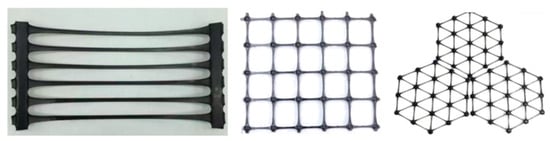
Figure 1.
Conventional uniaxial, biaxial, and triaxial geogrids.
Design optimization methods for geogrids typically encompass size, shape, and topology optimization, with topology optimization considered the most advanced approach. Since the introduction of the homogenization method by Bendsoe and Kikuchi in the 1980s [6], which marked a new phase in topology optimization design research, a variety of distinctive topology optimization methods have been subsequently proposed. The Variable Density Method, derived from the homogenization approach, introduces a hypothetical material whose density can vary continuously between 0 and 1. The density is treated as the topological design variable, and an empirical relationship is used to describe the corresponding variation in elastic modulus, effectively transforming the complex problem of structural topology optimization into the central task of determining the optimal material distribution [7,8,9,10,11,12]. The physical foundation of this method was rigorously demonstrated by Bendsoe and Sigmund [13]. Due to its clear and concise physical concept, the Variable Density Method has been integrated into major commercial CAE software (ANSYS 2023, Abaqus 2022) and is widely used in continuum structural topology optimization.
In the field of topology optimization, Paiva et al. used ABAQUS to establish a three-dimensional model of a biaxial geogrid [14]. They analyzed its response under uniaxial and biaxial tensile loading and validated the model using experimental data. Subsequently, they employed the TOSCA module for topology optimization, achieving a 53% reduction in structural volume with only a 3% decrease in load-bearing capacity. Wang and Zhu applied continuum topology optimization technology to the configuration design of spatial thin shells, and taking hyperbolic paraboloid shells and spherical thin shells as subjects, they conducted topology optimization research under static loading [15]. Based on the SIMP variable density method, an optimization model was established and solved using the Optistruct 2021 software platform. By analyzing the topological configurations and their mechanical performance under different parameters, the optimal control parameters and corresponding thin-shell topological forms for specific working conditions were determined. The Optistruct software platform incorporates efficient optimization algorithms and offers straightforward computation [16]. It possesses notable advantages, including the ability to generate high-quality topological forms and suitability for the topology optimization of geogrid structures.
Regarding how to determine the performance of geogrids, Dong et al. employed FLAC2D numerical simulations to analyze the impact of construction damage on the mechanical properties of a specific biaxial geogrid [17]. Their study found that damage led to a significant reduction in both tensile strength and stiffness, with the strength reduction factor varying between 1.00 and 3.71 depending on the severity of the damage. Furthermore, Dong et al. conducted numerical simulations on geogrids with rectangular and triangular apertures using FLAC6.0 software [18]. Their results indicated that the triangular-aperture geogrid, due to its isotropic mesh structure, exhibited more uniform tensile stiffness and strength distribution compared to conventional rectangular-aperture geogrids. Discrete element software has been widely used to study the interaction between reinforcement and soil. Du et al. investigated the effects of four different boundary condition combinations on the geogrid–soil interface characteristics [19]. Chen et al. employed particle flow code to study the meso-mechanical properties of geogrid deformation [20]. Ma et al. utilized pull-out tests and numerical simulations to reveal the influence of geogrid mesh shape and aperture ratio on the reinforcement–sand interface mechanism from a mesoscopic perspective, aiming to determine the optimal mesh design [21].
Previous studies on geogrids have often employed stiffness-maximization configurations under single, idealized tensile conditions (e.g., uniaxial or biaxial tension), which fail to adequately capture the complex stress states experienced by geogrids in real reinforced soil structures. In this research, multi-condition and multi-objective equivalent optimization models were established based on the mechanical characteristics of three types of geogrids. Furthermore, this paper introduced a “minimum member size” constraint. Through parametric analysis, it was determined that this size should be approximately 2–2.5 times the mesh element size, and its influence was systematically analyzed. This directly ensures that the width of the optimized ribs meets the minimum rib width requirements imposed by actual manufacturing processes, thereby advancing the optimization results a significant step from “conceptual configurations” toward “manufacturable configurations”. More importantly, this study establishes a complete analytical chain, encompassing “topology optimization design” to “macro-scale tensile performance numerical validation (FLAC3D)” to “meso-scale soil–reinforcement interface interaction validation (coupled PFC3D–FLAC3D pull-out simulation)”. It verifies the effectiveness of compliance-minimization-based optimization for the tensile performance of geogrids and further examines whether such optimization also enhances performance.
Therefore, the variable density method was adopted in this study for continuum structural topology optimization and the Optistruct optimization software platform, using structural compliance minimization as the optimization objective and the relative element density as the design variable, topology optimization under a single load condition was performed for the uniaxial, biaxial, and triaxial geogrids, subject to a prescribed volume-fraction constraint. The effects of the volume fraction constraint, minimum member size, symmetry constraints, and post-processing density threshold on the optimization results were evaluated. Based on these analyses, the optimal geogrid configurations were obtained. To further verify the performance of the topologically optimized geogrid, a comparative analysis of the performance differences between the new topologically optimized geogrid and conventional geogrids was conducted through FLAC3D numerical simulation, aiming to validate of the optimized design. Subsequently, this study employed PFC3D–FLAC3D coupled modeling to simulate pull-out tests at the geogrid–sand interface, investigating the mechanism by which geogrids of different shapes constrain the soil. The results demonstrate that the new topologically optimized geogrid performs excellently in terms of interface friction characteristics. The topology-optimized new geogrid demonstrated excellent performance in both tensile resistance and interfacial shear resistance, significantly enhancing the overall properties of geogrids. This provides an important reference for the design of new-generation geogrids.
Table 1 presents the constitutive models and parameters such as elastic modulus and Poisson’s ratio set for the geogrid in OptiStruct, FLAC3D, and PFC3D–FLAC3D, respectively. The geogrid was modeled using a linear elastic constitutive law, and this study was conducted within a “small-strain, linear-elastic” framework. In OptiStruct (ν = 0.42), the typical experimental value for PP material was adopted, aligning with physical reality. In FLAC3D (ν = 0.30) and PFC3D (ν = 0.30), the values were adjusted to those more commonly used in geotechnical numerical analysis. For thin-shell or geogrid structures under in-plane tension-dominated conditions [15], the influence of Poisson’s ratio on overall stiffness and stress distribution is secondary. Altering Poisson’s ratio does not reverse the primary load transfer paths derived from material layout optimization. Furthermore, in FLAC3D, a lower Poisson’s ratio helps enhance the numerical stability of the explicit dynamic relaxation algorithm, preventing non-physical oscillations during simulations of large deformations or complex contacts. This adjustment is based on considerations of numerical robustness and does not affect the comparative evaluation of relative performance among different geometric configurations in this study.

Table 1.
Properties of polypropylene (PP) materials used in each numerical simulation stage.
2. Topology Optimization of Geogrids
2.1. Structural Topology Optimization Algorithms
This study considered the geogrid as the research object and performed topology optimization based on the continuum structure optimization method [22], which discretizes the material within the geogrid structure’s optimization domain into a finite number of elements. The Variable Density Method [23] is one of the most widely used and mature optimization approaches, known for its high computational accuracy and rapid convergence. Topology optimization based on the Variable Density Method utilizes finite element analysis to divide the optimization area of the structural component into multiple finite elements. During the solution process, the “element density” of each within the design space of the finite element model is treated as a design variable, and the relative density of all elements was constrained to the range from 0 to 1. Elements with densities between 0 and 1 represent a relatively ambiguous topological configuration. To mitigate the influence of these intermediate densities on the final material distribution of the optimized structure, a penalty factor p is introduced. The Solid Isotropic Material with Penalization (SIMP) method is commonly employed within the variable density framework [24]. The interpolation model for the SIMP method is expressed as:
where xi represents the element density of the i unit, E(xᵢ) denotes the elastic modulus of the i unit, and p is the penalty factor. The parameters Emin and E0 correspond to the elastic moduli of materials with relative element densities approaching 0 and 1 within the design domain, respectively. To prevent singularity of the stiffness matrix, Emin is typically assigned a value of E0/1000.
Figure 2 illustrates the influence of different penalty factors p on the SIMP Equation (1). The ordinate Eᵢ represents the ratio of E(xᵢ) to E0, denoting the relative elastic modulus. A larger value of p accelerates the convergence of the penalized relative elastic modulus Eᵢ towards 1 and 0, indicating that intermediate material densities in the optimized structure also converge toward these extremes. Therefore, it is necessary to select a suitable value for the penalty factor p, as a higher value does not necessarily yield a more precise optimization outcome. Wang and Zhu [15], in their topology optimization of continuum thin-shell structures, concluded that when the penalty factor p is set to 5.0, the model achieves a more thorough topology optimization, exhibits overall greater regularity, and ultimately attains the minimum compliance. Therefore, in this paper, the penalty factor p for the geogrid structure was taken as 5.0.
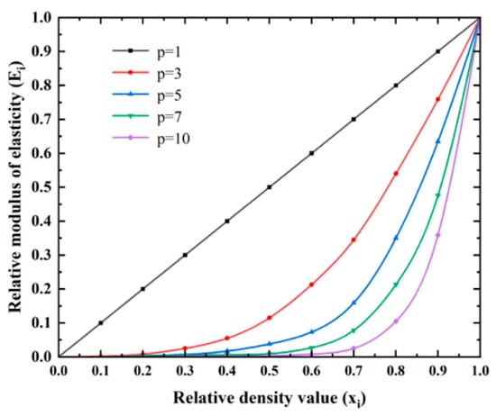
Figure 2.
The impact of p in the SIMP interpolation model.
2.2. Mathematical Model of Structural Topology Optimization
This study investigated the topology optimization of shell structures under static loads, aiming to maximize structural stiffness. Under the constraint of volume fraction, the mathematical equation for the topology optimization of continuum structures is as follows:
where x is the optimization design variable, representing the vector of relative densities of each element; i is the number of elements; Ω is the set of optimization design variables; F is the external load matrix of the structure; U is the displacement matrix of the structure; K is the global stiffness matrix of the structure; V(xi) is the actual volume function of the structure; V∗ is the volume constraint fraction value set for optimization; C(x) is the structural compliance matrix formed by the function of the design variable x. The topology-optimized structure should satisfy the static strength design criteria and stiffness criteria. Therefore, by setting volume fraction constraints, the material retention ratio is maximized while meeting the stiffness requirements.
The SIMP method is applied to the topology optimization of the geogrid, and the optimization process is shown in Figure 3.
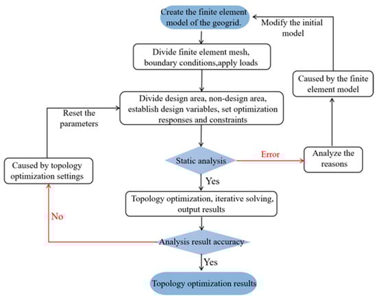
Figure 3.
Flowchart of geogrid topology optimization.
2.3. Finite Element Model of Geogrid Structure
Table 2, Table 3 and Table 4 provide the index properties of three types of plastic geogrids as Transportation Industry Standard [25]. In the software Optistruct, the elastic modulus E of the material is determined based on the tensile stress at 5% strain provided in Table 1, Table 2 and Table 3, with the Poisson’s ratio μ set to 0.42 and the density ρ to 900 kg/m3 for the polypropylene material. Select 2D shell elements with a shell thickness of 2.5 mm, use quadrilateral meshes, and set the average size to 2 mm. Topology optimization is performed on the topological configurations of uniaxial, biaxial, and triaxial geogrid structures, assuming the material always remains in the elastic range during loading [26].
Table 2.
Physical indicators of uniaxial geogrids.
Table 3.
Physical indicators of biaxial geogrids.
Table 4.
Physical indicators of triaxial geogrids.
Based on the dimensional parameters of conventional geogrids, topology optimization models were developed for the structures of three geogrid types. Figure 4a illustrates the finite element model of the topology optimization for a uniaxial geogrid. The model dimensions correspond to those of a commercially available conventional uniaxial geogrid, with a length of 465 mm and a width of 180 mm. The central point of the model (marked in Figure 4a) is fully fixed (constraining all six degrees of freedom: UX, UY, UZ, ROTX, ROTY, ROTZ). A uniformly distributed load of 10 kN/m, equivalent to 4.65 kN, is applied in the positive and negative x-directions to the nodes on both width sides of the model. To enhance the transverse tensile strength of the uniaxial geogrid, concentrated tensile loads of ±2.0 kN each along the y-axis are applied to three nodes at the center of the transverse edges (regions ② and ⑤), as well as to three mesh nodes located three nodes away from the left and right edges (regions ①, ③, ④, and ⑥). An X-Z plane symmetry constraint is imposed to ensure the optimized configuration is symmetric in the transverse direction.
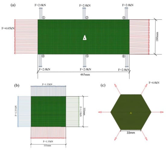
Figure 4.
Finite element models of geogrids: (a) Finite element model of the uniaxial geogrid; (b) Finite element model of the biaxial geogrid; (c) Finite element model of the triaxial geogrid.
Figure 4b illustrates the topology optimization structure for a biaxial geogrid. Conventional biaxial geogrids consist of uniformly distributed transverse and longitudinal ribs, forming regular square apertures. The model has a length and width of 11.1 cm, with a thickness of 2.5 mm. The nodes along the model’s vertical symmetry axis (Y-axis) are constrained in UY and UZ, while the nodes along the transverse symmetry axis (X-axis) are constrained in UX and UZ. The central node of the model is fully fixed, constraining all six degrees of freedom: UX, UY, UZ, ROTX, ROTY, and ROTZ. A uniformly distributed load of 12 kN/m, equivalent to 1.33 kN, is applied to the nodes on the periphery of the shell, subjecting the model to a biaxial symmetric tensile state.
Figure 4c presents the finite element model depicting the load state for the topology optimization of a triaxial geogrid. Utilizing the model’s symmetry during meshing, the hexagonal model has a side length of 3.3 cm. The central node of the hexagon is fully constrained in all six degrees of freedom: UX, UY, UZ, ROTX, ROTY, and ROTZ. All other nodes in the model are constrained in UZ. Symmetrically concentrated tensile loads, each with a magnitude of 4.0 kN, are applied along the edges in the 0°, 60°, and 120° directions (oriented radially outward along their respective angles). Leveraging the cyclic symmetry of the hexagon, X-Z and Y-Z plane symmetry constraints are applied during optimization to simplify the calculations. The magnitude of the applied symmetrical concentrated forces is not dependent on the tensile force itself, but rather on the chosen loading method and direction.
To demonstrate that the topology optimization results are independent of the mesh, a mesh sensitivity analysis was conducted for the biaxial geogrid. Three different mesh sizes (coarse: 4 mm, baseline: 2 mm, fine: 1 mm) were selected, and topology optimization was performed under identical parameters (‘p’ = 5.0, Vfrac = 0.30, Mmindim = 5.0). Table 5 compares the optimized configuration shapes and structural compliance.
Table 5.
Mesh sensitivity comparison analysis.
The results show that as the mesh size was refined from 4 mm to 1 mm, the primary load transfer paths in the optimized configuration remained consistent, and the variation in compliance values was less than 5%. This indicates that the optimization results had stabilized. The baseline mesh (2 mm) achieved a good balance between computational efficiency and result accuracy. Therefore, all optimizations presented in this paper used this mesh size.
In this study, a penalty factor of ‘p’ = 5.0 was used for the topology optimization of uniaxial, biaxial, and triaxial geogrids. This value references the optimization research on thin-shell structures by Wang and Zhu [15], which has been verified to achieve a good balance between material penalization and convergence stability. Parameters such as the volume fraction Vfrac and the minimum member size Mmindim were adjusted based on the initial geometric characteristics and load-bearing features of each type of geogrid. The specific values and justifications are provided in the explanations below.
2.4. Parametric Analysis of Geogrid Structure Topology Optimization
Key parameters in structural topology optimization, such as volume fraction, minimum member size, maximum number of iterations, checkerboard control, and convergence tolerance, strongly influence the characteristics of the optimized structure. To achieve a satisfactory structural configuration, it is necessary to analyze the influence of these parameters and select appropriate values for the optimization process [27]. This paper first established a set of parameter standards A, and then progressively determined the most suitable parameters for optimizing the geogrid shape during the optimization process. The parameter standard set A is specifically defined as: volume fraction constraint Vfrac = 0.3, minimum member size Mmindim = 5 mm, symmetric constraint applied, and convergence tolerance set to 0.5%. This study investigated the effects of three key parameters, including volume fraction, symmetry constraints, and minimum member size, on the topology optimization of geogrid structures. The control variable method was employed for the analysis, where only one parameter is altered at a time while keeping the others constant. Table 6 lists the final parameters used in the topology optimization for the three configurations: uniaxial, biaxial, and triaxial geogrids.
Table 6.
Summary of topology optimization parameters for geogrids.
2.4.1. Volume Fraction
The distribution of material and the formation of shapes in the optimized topology are closely related to the value of the volume fraction. Therefore, selecting an appropriate range for the volume fraction is particularly important, as it helps ensure that the geogrid retains adequate and reasonably distributed regions after topology optimization. The material usage in the topologically optimized geogrid should be less than that in conventional geogrids, thereby achieving performance superiority on the basis of lightweight design. Due to differences in the stretching process and aperture design, the volume ratio of conventional stretched geogrids typically ranges between 0.2 and 0.5 [22]. Taking the topology optimization of a biaxial geogrid as an example, the volume fraction Vfrac in the standard parameter set was sequentially set to 0.4, 0.35, 0.3, 0.25, 0.2, and 0.15 to investigate the influence of the volume fraction constraint on the topological configuration of the structure. Figure 5 shows the density nephogram and iteration results of the geogrid structure under different volume fraction constraints.
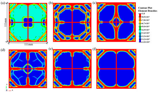
Figure 5.
Density contour of the optimized geogrid structure under different volume fraction constraints for the biaxial geogrid: (a) Vfrac = 0.40; (b) Vfrac = 0.35; (c) Vfrac = 0.30; (d) Vfrac = 0.25; (e) Vfrac = 0.20; (f) Vfrac = 0.15.
As shown in Figure 5, when the volume constraint Vfrac was 0.4, most material elements in the optimized structure exhibited intermediate density values (0–1), resulting in an unreasonable optimization outcome. As the volume fraction constraint decreased from 0.35 to 0.2, the material distribution in the geogrid structure gradually formed clear load-transfer paths, with more material element densities converging toward 0 and 1. Specifically, when Vfrac was 0.3, the aperture shape and distribution appeared most uniform and regular, demonstrating superior structural integrity. However, at a volume constraint of 0.15, well-defined load-transfer paths failed to develop. In conclusion, for the biaxial geogrid, the most reasonable topological configuration is achieved when the volume fraction constraint Vfrac fluctuates around 0.3.
2.4.2. Symmetry Constraint
Symmetry constraints were categorized into one symmetry plane, two symmetry planes, three symmetry planes, and cyclic symmetry. Taking the biaxial geogrid structure as an example, selecting two-plane symmetry ensures that the optimized material is symmetrically distributed along both the X-Z and Y-Z planes. Referencing the standard parameter set, only the symmetry constraint setting is modified. Figure 6 shows the structural topological configurations obtained without and with symmetry constraints, providing a comparative analysis of their influence on the topological configuration.
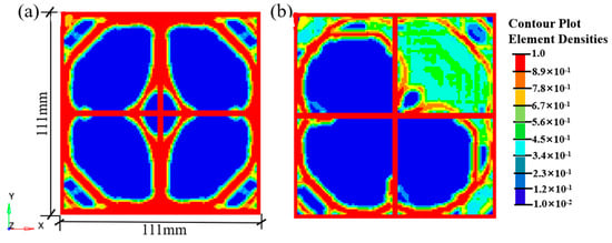
Figure 6.
Comparison of the influence of symmetry constraints on topological configurations: (a) Symmetry constraint; (b) Non-symmetry constraints.
Figure 6 illustrates that when symmetry constraints are applied, a highly symmetrical topological configuration can be achieved. The material was more rationally distributed, resulting in a regular and uniform overall geometry with smoother edges. In contrast, without symmetry constraints, the configuration exhibited intermediate density values, uneven edges, and failed to develop a well-defined topological structure in the central region.
2.4.3. Minimum Member Size
During the continuum topology optimization design process, a minimum member size constraint can be implemented to achieve a more uniform material distribution. The minimum member size (Mmindim) constraint is a crucial manufacturability constraint in continuum topology optimization. Its role is to control the “minimum feature width” of any material region within the optimized structure. For geogrids, this parameter prevents the optimization results from including extremely thin, easily breakable ribs or “point-like” connections. While these slender components may exhibit high stiffness in macroscopic mechanical models, they are highly susceptible to failure in real materials due to micro-defects, stress concentration, or fatigue. Consequently, they become weak points in the structure, compromising the overall load-bearing capacity and durability of the geogrid. Based on the pre-processing mesh size and the Transportation Industry Standard [25], minimum member sizes of 4.5 mm, 5 mm, 5.5 mm, and 6 mm were respectively set to analyze the optimization effect of the geogrid structure. The resulting maximum displacements and iteration steps are presented in Table 7.
Table 7.
Maximum displacement and iteration steps corresponding to different minimum member sizes.
As summarized in Table 7, as the minimum member size Mmindim increases, the maximum displacement after optimization also increases correspondingly. Figure 7 illustrates the impact of varying Mmindim from 4.5 mm to 6.0 mm on the optimized configuration of the biaxial geogrid. In OptiStruct, Mmindim indirectly defines the scale of the “minimum detail” allowed in the material distribution by influencing the effective radius of the density filter. Increasing Mmindim means that the optimization algorithm will suppress or merge fine features smaller than this scale when searching for the material layout.
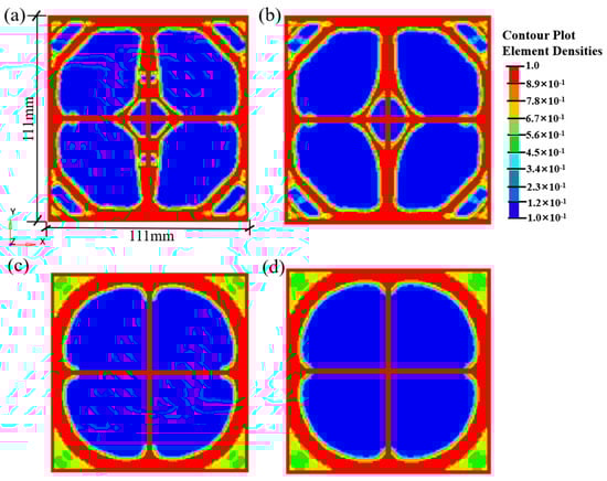
Figure 7.
Density contour of geogrid structures with different minimum member sizes after optimization: (a) Mmindim = 4.5; (b) Mmindim = 5.0; (c) Mmindim = 5.5; (d) Mmindim = 6.0.
When Mmindim is set to 4.5 mm, which is approximately twice the mesh size, the algorithm retains a strong capability to preserve fine features. As shown in Figure 7a, the result may contain numerous details close to the mesh scale, sometimes exhibiting “jagged” trends. Although theoretically this may yield a slightly better compliance value (see Table 7), these irregular, minute features are extremely difficult to manufacture and are prone to becoming crack initiation points under load. When Mmindim is set to a moderate value (e.g., 5.0 mm), this value, which is about 2.5 times the mesh size (2 mm), effectively preserves clear, macroscopic load transfer paths. As shown in Figure 7b, the resulting topological configuration features smooth and continuous ribs with regularly shaped holes. This not only meets the mechanical performance requirements (with compliance values close to optimal, see Table 7) but also ensures good manufacturability. When Mmindim is set too high (e.g., 5.5 mm, 6.0 mm), excessive scale filtering overly smoothens structural details, causing originally clear load transfer paths to become blurred, bulky, or even resulting in material accumulation in non-critical areas. As shown in Figure 7c,d, the clarity of the configuration diminishes, which contradicts the original goals of lightweight design and efficient load transfer, leading to a significant deterioration in structural compliance (increased displacement in Table 7). Based on the above analysis, we selected Mmindim = 5.0 mm as the optimal value.
2.5. Post-Processing and Results of Topology Optimization
The optimized topological configuration is obtained by leveraging the visualization capabilities of HyperView and by adjusting the element density threshold to generate corresponding isosurfaces. The selected density threshold significantly influences structural clarity, the distribution of elements, and the validity of the optimization results. Specifically, when the threshold is set to D, elements with densities less than or equal to D are excluded, while elements with densities greater than D are retained, thereby defining the final optimized geometry. The density threshold has a significant impact on the total mass, displacement, and stress of the optimized structure; therefore, selecting an appropriate threshold is crucial. Figure 8 shows the density cloud diagrams of the biaxial geogrid structure for D values of 0.3, 0.4, 0.5, 0.6, 0.7, and 0.8.
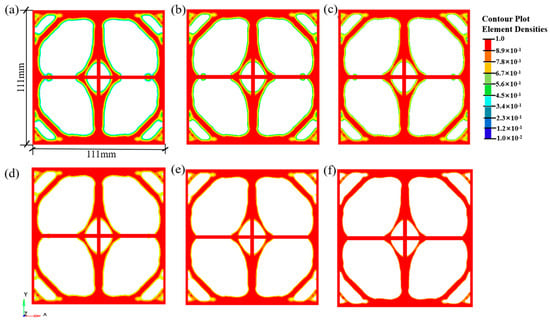
Figure 8.
Density contour plot corresponding to different thresholds; (a) D = 0.3; (b) D = 0.4; (c) D = 0.5; (d) D = 0.6; (e) D = 0.7; (f) D = 0.8.
As the element density threshold D increases, the amount of material retained after structural optimization decreases. However, an excessively high density threshold leads to discontinuous structural components and localized stress concentration, as shown in Figure 8f. This study exported geometric models for the biaxial geogrid optimized under a volume fraction Vfrac = 0.3, applying density thresholds D ranging from 0.3 to 0.8. For each model, the following metrics were calculated: Relative mass (m/m0): The ratio of the exported model’s mass to the mass of the original design domain. Relative compliance (C/C0): The model was imported into FLAC3D, subjected to the same biaxial tensile loads used in the optimization, and its compliance was calculated. This value was then compared to the compliance of the model at D = 0.3. Maximum Principal Stress (σmax): The maximum principal stress value extracted from the same FLAC3D tensile analysis. As shown in Figure 9, within the D range of 0.4 to 0.6, the structures achieved significant lightweighting while maintaining good connectivity and manufacturability. Simultaneously, the increases in compliance and stress were controlled at acceptable, relatively low levels (<15%). At D = 0.5, an optimal balance between performance retention and lightweighting was achieved.
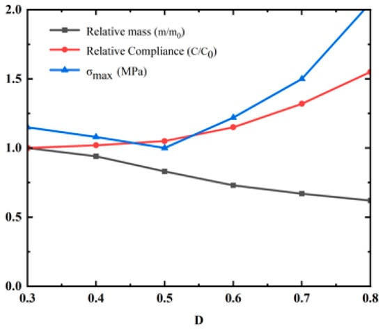
Figure 9.
Performance trade-off curves for biaxial topology optimized geogrids under different density thresholds.
Based on the above methodology, Laplace smoothing was applied using the Ossmooth module to achieve smoother boundaries. To ensure a defect-free conversion from density contour maps to CAD models, the following steps are implemented after exporting the smoothed Stl or mesh file, using Rhino’s mesh analysis tools and custom scripts to check the mesh quality. If the inspection reveals that local smoothing has caused “necking” or insufficient thickness in specific areas, the smoothing parameters are adjusted (by reducing the number of iterations), or the density threshold for that region is slightly modified manually. The model is then re-smoothed and re-inspected iteratively until all requirements are met. This ultimately yields the results shown in Figure 10.
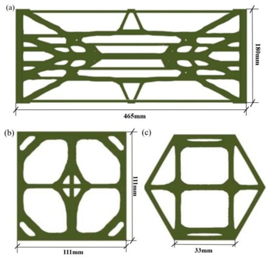
Figure 10.
Optimized topological configurations of three geogrids at a density threshold of 0.70. (a) Topologically optimized configuration of uniaxial geogrid; (b) Topologically optimized configuration of biaxial geogrid; (c) Topologically optimized configuration of triaxial geogrid.
To verify whether the material usage of the topologically optimized geogrid is less than that of conventional geogrids, modeling software was used to reconstruct the above-mentioned geogrids. The aperture areas of the geogrids were identified, with specific data provided in Table 8. The aperture areas of the topologically optimized geogrids were consistently larger than those of the conventional geogrids, and the three types of geogrids achieved weight reductions of 7%, 10%, and 12%, respectively, indicating that the material regions in the optimized geogrids were smaller than those in the conventional ones. This confirms the lightweight nature of the topologically optimized geogrids.
Table 8.
Comparison of material distribution between conventional geogrids and topologically optimized geogrids.
3. Numerical Validation of Geogrid Tensile Performance
To validate the tensile strength of the topologically optimized geogrid configuration, this study utilized the FLAC3D finite difference software to conduct tensile tests. The superiority of the tensile performance of the topologically optimized geogrid was verified by comparing its tensile strength with that of conventional uniaxial, biaxial, and triaxial geogrids.
3.1. Model Parameters and Establishment
Using Rhino7 software and its built-in Griddle parametric platform, three-dimensional geometric models of the geogrids obtained through topology optimization were established, accurately replicating the geogrid models at a 1:1 scale. Based on the prior topology optimization of the three types of tensile geogrids, models were established for both conventional and topologically optimized designs. The uniaxial geogrids measured 460 mm in length and 150 mm in width, the biaxial geogrids measured 250 mm in length and 222 mm in width, and the triaxial geogrids measured 330 mm in length and 245 mm in width. The thickness of all geogrid models was set to 2.5 mm, and all models were verified as closed, error-free solids. Following the meshing process, the grid was exported in a format compatible with FLAC3D for subsequent numerical analysis. The parameters were configured as shown in Figure 11. The figure illustrates the resulting model after meshing and import into FLAC3D 7.0.
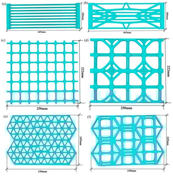
Figure 11.
Geogrid models imported into FLAC3D: (a) Conventional uniaxial geogrid; (b) Topologically optimized new uniaxial geogrid; (c) Conventional biaxial geogrid; (d) Topologically optimized new biaxial geogrid; (e) Conventional triaxial geogrid; (f) Topologically optimized new triaxial geogrid.
The superior tensile performance of the topologically optimized geogrid was validated through the use of two loading methods: strain-controlled and force-controlled loading. The tensile performance was evaluated by analyzing the principal stress distribution and stress–strain response of both conventional and new geogrids under identical working conditions.
In strain-controlled loading, fixed constraints were applied to the grid, and tensile displacement was applied to the nodes at the free end of the geogrid. The loading stopped when the geogrid reached a tensile strain of 5%, resulting in the stress distribution of the geogrid. In force-controlled loading, a tensile force was applied to the geogrid based on its stable state. The tensile performance was then analyzed by comparing the displacement and stress responses of the geogrid. The specific working conditions for measuring the tensile performance of the geogrid are shown in Table 9.
Table 9.
Configuration of the numerical simulation working conditions for the geogrid under tension.
In this study, a linear elastic constitutive model was employed for the geogrids in both OptiStruct and FLAC3D. The primary objective was to compare the relative performance between conventional and topology-optimized geogrids, encompassing stiffness, uniformity of stress distribution, and load transfer efficiency. These performance metrics can be adequately evaluated and contrasted within the elastic range. The stress concentration factor calculated from linear elastic analysis (reflected in high-stress areas within stress contour plots) serves as a key indicator for predicting potential sites of fatigue crack initiation or brittle fracture onset. A significantly higher peak elastic stress directly suggests that the corresponding region would be the first to yield or fail under cyclic or ultimate loading. Therefore, the more uniform elastic stress distribution and reduced peak stress observed in the optimized geogrid can be directly interpreted as indicative of its superior potential for fatigue and fracture resistance.
3.2. Model Validation
To simulate laboratory tensile tests, Dong and Han [18] selected biaxial geogrids based on the aperture sizes of commercially available products and determined a mesh size of 330 mm × 200 mm. The mesh was fixed to prevent movement in both the x and y directions. An equal velocity at 5 × 10⁻⁸ m/step was applied horizontally on each node on the right boundary with an increasing magnitude until the failure of the sample. The right boundary could only move in the x direction but not in the y direction. The right boundary did not allow any rotation either. This boundary was created to simulate a clamp in a laboratory test. The top and bottom boundaries of these meshes were free for displacements in the x and y directions. In this paper, the same method was used, applying tensile force to conventional biaxial geogrids with identical mesh dimensions in the 0°and 90°directions, respectively, and the numerical simulation results were compared. Figure 12 shows the comparative results, indicating that for both the 0° and 90° directions, the numerical results exhibited reasonable consistency in terms of tensile stiffness and ultimate tensile strength. The horizontal line denotes the peak load capacity of the geogrid. After this point, the geogrid may retain some load-carrying capacity, but at a lower level. Tensile stiffness and ultimate tensile strength are key parameters in geogrid tensile tests and are used in design.
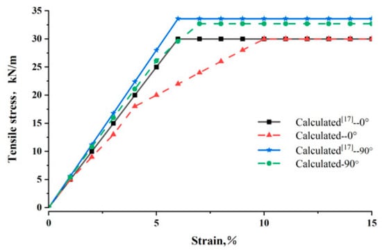
Figure 12.
Comparison between the numerical results and reference [17] for the biaxial geogrid under tension in 0° and 90°directions.
3.3. Analysis of Numerical Simulation Results
According to the maximum tensile stress theory, brittle fracture occurs when the maximum principal stress reaches the material’s uniaxial tensile strength. Therefore, a geogrid becomes more prone to failure when subjected to higher stress levels. Conventional uniaxial geogrids demonstrate high longitudinal strength. Under identical loading conditions, where all nodes on the left boundary are constrained in the x, y, and z directions and a horizontal tensile force is applied to the right boundary while allowing free movement in the x-direction, Figure 13 shows the stress distribution and displacement contours for both geogrid types. Under the same tensile force, the lateral displacement of the conventional geogrid is 0.0148 m, while that of the topologically optimized geogrid is 0.0136 m. The maximum principal stress in the conventional geogrid is 3.05 × 10⁷ Pa, highly concentrated on each transverse rib, making failure likely to initiate at these stress concentration points and propagate rapidly. In contrast, the optimized geogrid has a slightly lower maximum principal stress of 3.0 × 10⁷ Pa, concentrated in specific areas of the central transverse rib. Its stress distribution forms a continuous, root-like load-transfer path, ensuring smooth force flow. Failure may start in the central transverse rib, but the structural design helps impede or delay rapid crack propagation. Additionally, the surplus material on both sides of the central section in the optimized geogrid, though not directly contributing to transverse tensile resistance, enhances longitudinal tensile strength.
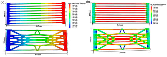
Figure 13.
Stress diagram of uniaxial conventional and uniaxial topologically optimized geogrids under transverse tensile load: (a) Comparison of displacement diagrams between conventional uniaxial geogrid and new geogrid; (b) Comparison of maximum principal stress distribution diagrams between conventional uniaxial geogrid and new geogrid.
When constraints are applied at the center of the central transverse rib of both geogrids, and three identical tensile loads are applied at the top and bottom ends (both at the edges and the center), the resulting stress and displacement contours are shown in Figure 14. The maximum displacement of the conventional geogrid was 0.09 m, significantly higher than the 0.018 m of the optimized geogrid. The conventional geogrid also showed localized displacement concentrations, whereas the optimized geogrid exhibited uniform deformation during stretching, with more coordinated and even overall deformation. Its unique topology effectively restrains out-of-plane instability, ensuring stability during tension. Furthermore, the conventional geogrid’s maximum principal stress (3.5 × 10⁷ Pa) exceeded that of the optimized geogrid. The stress distribution in the optimized geogrid was more uniform and continuous, with efficient force flow paths that distribute tensile stress to other transverse ribs. In contrast, only the side ribs in the conventional geogrid bore the longitudinal tensile stress, resulting in an uneven stress distribution.
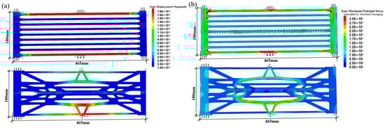
Figure 14.
Stress diagrams of uniaxial conventional and topologically optimized geogrids under combined transverse and longitudinal tensile loading: (a) Comparison of displacement diagrams between conventional uniaxial geogrid and new geogrid; (b) Comparison of maximum principal stress distribution diagrams between conventional uniaxial geogrid and new geogrid.
Thus, the topologically optimized uniaxial geogrid not only surpasses the conventional geogrid in transverse tensile performance but also demonstrates enhanced longitudinal tensile capacity, making it more adaptable to complex engineering scenarios. This further validates the rationality and efficiency of the topology optimization design.
The tensile performance of biaxial and triaxial geogrids was analyzed using the stress-controlled method. The central node of the geogrids was fixed in the x, y, and z directions. For the biaxial geogrid, a tensile force of 10 kN/m was applied in the 0° and 90° directions, while for the triaxial geogrid, a tensile force of 10 kN/m was applied in the 0°, 60°, and 90° directions. The stress distribution in both types of biaxial geogrids was highly uniform and optimal, the high-stress zones were no longer confined to discrete nodes but were distributed along smooth, continuous paths, forming an efficient force flow transmission network. However, by comparing the displacement and minimum principal stress under identical tensile loads, it was observed that the displacement of the conventional geogrid was 4.89 × 10⁻³ m, while that of the new biaxial geogrid was 2.91 × 10⁻³ m, indicating that the displacement of the new geogrid was smaller (Figure 15). The minimum principal stress of the conventional geogrid was 2.48 × 10⁶ Pa, whereas that of the new biaxial geogrid was 1.00e6 Pa, also lower than that of the conventional geogrid. These results demonstrate that the new biaxial geogrid exhibits superior tensile performance compared to the conventional one.
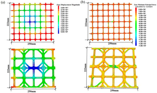
Figure 15.
Stress diagrams of biaxial conventional and topologically optimized geogrids under biaxial tensile loading: (a) Comparison of displacement nephograms between conventional biaxial geogrids and new bidirectional geogrids. (b) Comparison of minimum principal stress distribution diagrams between conventional biaxial geogrid and new geogrid.
The triaxial geogrid was subjected to tensile loading in the 60° direction. The stress contour of the conventional triaxial geogrid (Figure 16) shows that due to the advantages of its triangular structure, the stress distribution was more uniform compared to that of biaxial geogrids. However, significant stress concentration remained evident at the core nodes where multiple ribs converged. The optimized design significantly mitigates this stress concentration by eliminating sharp corners and improving material distribution. Given that the tensile performance of triaxial geogrids is further enhanced in the diagonal direction, this paper presents the stress and strain distributions of conventional and new triaxial geogrids in the 60° direction. The contour plots indicate that under identical loading conditions, the maximum displacement and minimum principal stress of the new triaxial geogrid were both lower than those of the conventional triaxial geogrid. For the triaxial geogrid, the topology optimization potentially enhances its load-bearing efficiency in specific dominant directions without compromising isotropy. Through improved nodal design, it achieves superior overall performance under multi-directional loading.
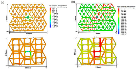
Figure 16.
Stress diagram of triaxial conventional and triaxial topologically optimized geogrids under 60° direction tensile load: (a) Comparison of minimum principal stress distribution diagrams between conventional triaxial geogrid and new geogrid. (b) Comparison of maximum principal stress distribution diagrams between conventional triaxial geogrid and new geogrid.
In summary, topology optimization demonstrates remarkable effectiveness in enhancing the tensile stiffness, strength, and stress distribution of geogrids. These performance improvements are achieved while maintaining or even reducing material usage, highlighting its significant potential for lightweight design and substantial economic value.
4. Numerical Simulation of Geogrid Pull-Out Test
4.1. Numerical Simulation and Validation of Pull-Out Test
The discrete element–finite difference coupling method has been widely used to simulate soil–structure interaction problems involving complex contacts and discontinuities [19,20,21]. Ali Asgari et al. [28], in their analysis of complex problems involving large deformations and soil–structure interaction, demonstrated through three-dimensional evidence from parallel finite element computations that robust numerical models are a prerequisite for revealing deeper mechanical mechanisms. Patrício, J.D. et al. [29] emphasized the fundamental importance of explicitly considering interaction mechanisms and conducting model validation in foundation design while accounting for soil–structure interaction. Drawing on this perspective, this study validated the effectiveness of the proposed coupling model by reproducing pull-out tests (Figure 16).
Bao emphasized in the study that when reinforcement materials move within soil [30], frictional resistance accounts for only 10% of the total resistance, while the embedment effect dominates, reaching up to 90%. This highlights the critical importance of studying the embedment performance of geogrid reinforcements. To investigate the influence of geogrid aperture shape and size on the interfacial strength of reinforced soil, Ma and Bai [21] employed a coupled Discrete Element Method (DEM) and Finite Difference Method (FDM) to simulate geogrid pull-out tests. They explored the effects of transverse rib arrangement and aperture ratio variations on the interface behavior and mechanisms of reinforced soil, examining the role of aperture shape and size for traditional biaxial geogrids, traditional triaxial geogrids, and two other new types of geogrids in standard sand. The soil test box measured 469 mm × 220 mm × 203 mm, with a total geogrid length of 530 mm. The geogrid was embedded at the mid-thickness of the soil layer, with an embedded length of 460 mm. After filling, the specimen was allowed to consolidate for 12 h. Finally, a rigid loading plate was placed on top of the fill, and normal pressure was applied via weights to conduct the pull-out test. The applied normal pressures σ were 15, 30, 60, and 90 kPa, with a pull-out speed of 0.5 mm/s.
This study adopted a coupled PFC3D–FLAC3D numerical method, using the same parameters as those in Ma and Bai’s [21] numerical simulation of pull-out tests. Normal stresses σ of 0, 60, and 90 kPa were applied to simulate pull-out tests on traditional biaxial geogrids. The numerical results from the coupled DEM–FDM simulation were compared with those from the coupled PFC3D–FLAC3D simulation, as shown in Figure 17. It was found that the relative error between the calculated results and the reference was less than 2%, indicating good agreement. Therefore, referencing the parameters from Ma and Bai allows for an accurate description of the mechanical behavior of geogrids with different shapes in soil. The specific parameters of the soil particles are presented in Table 10.
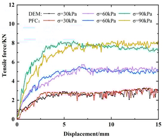
Figure 17.
Comparison between DEM simulation in reference [21] and PFC results in this study: pull-out force–displacement curves of biaxial geogrids under different normal stresses.
Table 10.
Mesoscopic parameters of soil particles.
4.2. Simulation of Pull-Out Tests for Geogrids with Different Shapes
Based on the aperture shapes and dimensions of the traditional biaxial geogrid, traditional triaxial geogrid, topologically optimized new biaxial geogrid, and new triaxial geogrid studied above, combined with the dimensions of the numerical soil model (length × width × height of 420 mm × 220 mm × 200 mm), four types of geogrids with dimensions of length × width × thickness of 485 mm × 131 mm × 2 mm were constructed, as shown in Figure 18.
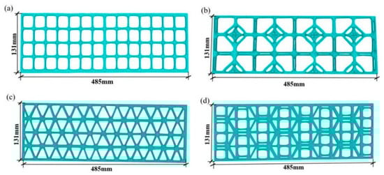
Figure 18.
Four types of geogrids with different aperture shapes: (a) Conventional biaxial geogrid; (b) Topologically optimized new biaxial geogrid; (c) Conventional triaxial geogrid; (d) Topologically optimized new triaxial geogrid.
In this study, ball elements in PFC3D were used to simulate standard sand particles, while zone elements in FLAC3D were employed to model the geogrid. Considering the requirements for simulation accuracy and computational efficiency, the particle size range selected for the soil in the model was 2.35–4.55 mm, with a uniform distribution and a median particle size (d50) of 3.47 mm. Mao et al. and Jiang indicate that the median particle size in the simulation should be less than 1/30 of the overall model size, and the number of particles in a 3D simulation model should exceed 40,000 to ensure that size effects do not compromise simulation accuracy [30,31]. Figure 19 illustrates the numerical simulation model for the pull-out test, which consists of 63,302 ball elements and 12,562 zone elements. A linear contact elastic model was assigned to govern the interactions between soil particles.
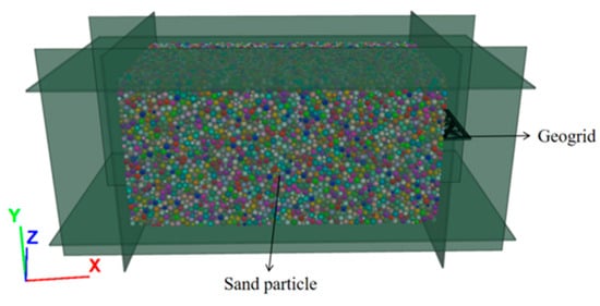
Figure 19.
Coupling model of PFC3D–FLAC3D for pull-out test: The dimensions of the numerical soil model (length × width × height of 420 mm × 220 mm × 200 mm) and the dimensions of the geogrids (length × width × thickness of 485 mm × 131 mm × 2 mm).
To ensure uniform contact within the sample, a servo function was used for pre-loading. A specific normal load was applied on the specimen by controlling the vertical movement of the loading plate. Once the specimen’s deformation stabilized, the geogrid was pulled out at a constant speed of 0.5 mm/s [31,32,33,34,35]. During this process, variations in pull-out force, displacement, and geogrid strain were recorded. During this process, changes in pull-out force, pull-out displacement, and geogrid strain were recorded. By comparing the interfacial shear resistance macroscopically exhibited at the reinforcement-soil interface of the new biaxial geogrid and new triaxial geogrid with that of the traditional biaxial geogrid and traditional triaxial geogrid, an analysis was conducted to determine whether the topologically optimized new geogrids demonstrated a superior reinforcement–soil interaction mechanism. Figure 20 shows cross-sectional views of the numerical models for the four types of geogrids.
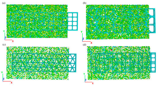
Figure 20.
Cross-sectional diagrams of numerical models for four types of geogrids. (a) Pull-out model of conventional biaxial geogrid; (b) Pull-out model of new biaxial geogrid; (c) Pull-out model of conventional triaxial geogrid; (d) Pull-out model of new triaxial geogrid.
4.3. Analysis of Pull-Out Test Simulation Results
As illustrated in Figure 21, under identical normal pressure conditions, the topologically optimized geogrids demonstrated significantly higher peak pull-out forces and residual pull-out forces compared to conventional geogrids with regular shapes. Importantly, this performance enhancement was achieved with approximately 5% less material used in the optimized structures. It is noteworthy that at a normal stress of 30 kPa, the peak pull-out forces of the optimized biaxial and triaxial geogrids increased by 3.6% and 3.2%, respectively, relative to their conventional counterparts. When the normal stress was increased to 60 kPa, the corresponding increases in peak pull-out force reached 20% for the optimized biaxial geogrid and 6.3% for the optimized triaxial geogrid. Under a normal stress of 90 kPa, the optimized biaxial and triaxial geogrids exhibited 11.3% and 23.4% higher peak pull-out forces, respectively, compared to the conventional geogrids. These results indicate that the aperture shapes of the topologically optimized geogrids are more effective in enhancing the shear strength at the sand interface. This demonstrates that topology optimization technology can create reinforced structures with higher mechanical efficiency.
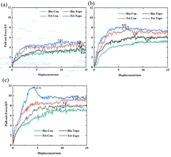
Figure 21.
Pull-out force–displacement curves of geogrids with different aperture shapes: (a) σ = 30 kPa; (b) σ = 60 kPa; (c) σ = 90 kPa.
4.4. Evaluation Metrics
Huang et al. [36] employed two methods, the interface resistance coefficient and the quasi-friction coefficient, to evaluate the interfacial friction performance between soil and double-twisted hexagonal mesh, geomembranes, and geogrids. Nie et al. [37] proposed that the pull-out friction coefficient serves as a comprehensive parameter characterizing the interfacial friction properties of aeolian sand–geogrid interfaces, while the interface resistance coefficient is a key indicator for analyzing the strength parameters of such interfaces. Both parameters are utilized for calculating and evaluating pull-out test results. This study adopted the calculation method for the resistance coefficient stipulated in the Chinese industry standard [25]: the ratio of the interfacial shear strength at the sand–geogrid interface to the shear strength of the sand itself. Based on this, key parameters for evaluating the interfacial friction strength were obtained. The peak shear strength of the sand–geogrid interface can be calculated using the following equation:
where
- Td = maximum pull-out force (kN);
- L, B = length and width of the geogrid used in the test (m);
- τ = shear strength at the soil–reinforcement interface (kPa).
Based on the pull-out test results, the relationship curves between normal stress and maximum shear stress for geogrids with different aperture shapes were plotted. Figure 22 shows the resulting shear strength envelope for the standard sand–geogrid interface, where the inclination angle of this line represents the interface friction angle φsg between the sand and the geogrid.
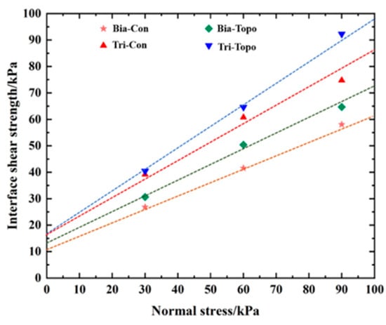
Figure 22.
Shear strength envelope line of the aeolian sand–geogrid interface.
Based on the following equation, the interface friction resistance coefficient fsg for geogrids with different aperture shapes was obtained, as shown in Table 11.
Table 11.
Resistance coefficients of sand–geogrid interfaces with different aperture shapes .
Table 12 summarizes the weight per area and material usage ratio of geogrids with different shapes. The material usage ratio was defined in this study as the ratio of the material used for a geogrid of a specific shape per area to that used for a conventional biaxial geogrid per area. This definition is considered to be of significant importance for the comprehensive comparison and selection of appropriate geogrids.
Table 12.
Material usage ratio of different geogrids.
To quantitatively analyze the reinforcement efficiency of geogrids with different shapes, a quantitative indicator is introduced here to compare the reinforcement efficiency of geogrids with different aperture shapes. For this purpose, Equation (5) is proposed:
η is the reinforcement efficiency index, and the index is mathematically defined as η = (fsg/f0)/(m/m0), where f/f0 is the interface resistance coefficient ratio (of a specific shape to a conventional biaxial geogrid) and m/m0 is the material usage ratio. This equation makes η a direct measure of the pull-out resistance effect generated per mass of geogrid material. An index value exceeding y (η > 1.0) denotes a design that offers superior efficiency for an equivalent material cost.
Table 13 presents the reinforcement efficiency of geogrids with different aperture shapes in standard sand. Considering material usage cost, the topologically optimized triaxial geogrid demonstrated the highest reinforcement efficiency, while the conventional biaxial geogrid showed the lowest. Specifically, the reinforcement efficiency of the topologically optimized biaxial and triaxial geogrids was 10% and 8% higher, respectively, than that of the conventional geogrids. The primary reason is that topological optimization inherently seeks the most effective load-transfer path under given loading conditions. The optimized aperture shapes eliminate unnecessary sharp corners and redistribute material to the primary load-bearing paths, thereby avoiding local stress peaks. In the numerical simulations, the pull-out resistance mainly originated from the interaction between the geogrid’s transverse ribs and the soil particles. The optimized shape likely creates more and more effective “anchoring points”, or the geometry of these points is more conducive to mobilizing a larger volume of soil during shearing. This enhances the macroscopic frictional resistance and interlocking force. Thus, the new topologically optimized geogrids exhibit significant potential and can be promoted for application in practical engineering.
Table 13.
Reinforcement efficiency of geogrids with different aperture shapes.
4.5. Comparative Analysis of Geogrid Comprehensive Performance
Table 14 summarizes the performance metrics of the three novel geogrids. Taking the biaxial geogrid as an example, a comprehensive comparison of performance parameters between conventional and topology-optimized designs shows that it achieved a 10% reduction in weight. Concurrently, stress concentration at critical locations was reduced by approximately 60%, and the interface pull-out resistance was increased by 20%. The research results demonstrate that the topology-optimized new geogrids perform well in both tensile and interface shear performance, significantly enhancing the overall performance of geogrids. This provides a valuable reference for the design of novel geogrids.
Table 14.
Quantitative comparison of performance metrics between conventional and topology optimized geogrids.
5. Conclusions and Discussion
5.1. Conclusions
This study introduces topology optimization technology into the design of geogrid aperture shapes. Subsequently, the employed “FLAC3D tensile analysis” and “PFC3D–FLAC3D coupled pull-out analysis” form a complementary multi-scale verification framework: the FLAC3D stage demonstrates that the optimized configuration possesses superior intrinsic mechanical properties (greater stiffness and more uniform stress distribution); the PFC3D–FLAC3D stage verifies that this superior intrinsic property translates into improved reinforcement efficiency within the complex system of soil–structure interaction. Through a combination of theoretical analysis, topology optimization, and multi-scale numerical simulation, the following main conclusions are drawn:
- Regarding Stress Concentration: The stress contour comparisons in Figure 13, Figure 14, Figure 15 and Figure 16 and the stress reduction data in Table 14 clearly show that the optimized configurations, by forming continuous and uniform load transfer paths, effectively disperse the highly concentrated stresses present at the nodes of conventional geogrids. The peak stress was reduced by up to approximately 59.7% (for the biaxial geogrid), significantly mitigating the stress concentration issue.
- Regarding Overall Performance Enhancement: More importantly, these improvements are not isolated. As indicated in Table 14, the reduction in material usage and the improvement in stress distribution collectively lead to increased structural stiffness and a higher interface reinforcement efficiency index (η). This demonstrates that topology optimization not only overcomes the limitations of conventional designs but also achieves synergistic performance enhancement.
5.2. Engineering Significance and Future Research Directions
The aforementioned methodological innovations have directly translated into design insights and performance enhancements with significant implications for engineering practice. It offers a concrete and actionable technical pathway for geosynthetic manufacturers to transition from trial-and-error aperture design to performance-driven “intelligent design”. This study quantitatively reveals that the specific geometries obtained via topology optimization feature smoother force flow transitions and reinforced nodes, achieving lightweighting while significantly enhancing peak interfacial shear resistance and reinforcement efficiency index η. This provides engineers with a new dimension beyond tensile strength, “shape efficiency”, for geogrid selection or customization, offering optimized solutions for balancing “lightweighting” and “high performance”.
Additionally, traditional rectangular and triangular hole molds are simple to process. Polymer geogrids primarily employ the stretch-forming process. Initially, sheets or strips with regular holes are formed by extrusion or injection molding. Then, under precise temperature control, they undergo uniaxial or biaxial stretching along specific directions, causing the holes to expand and form the final grid structure. However, the optimized smooth curve boundaries and irregular polygonal holes may increase the processing difficulty and cost of molds. However, with the widespread adoption of technologies such as 3D printing and laser cutting in mold manufacturing, producing molds with complex shapes is no longer an insurmountable obstacle. Although complex shapes may lead to higher initial mold costs, the resulting material savings and performance improvements offer significant long-term economic and technical benefits.
Author Contributions
Conceptualization, Y.C.; Methodology, Y.C. and L.C.; Software, L.C.; Formal analysis, S.S.; Investigation, L.C.; Data curation, L.C.; Writing—original draft, Y.C. and L.C.; Writing—review & editing, S.S., R.C. and X.Y.; Supervision, X.Z. and Y.M. All authors have read and agreed to the published version of the manuscript.
Funding
This research was funded by the National Natural Science Foundation of China, grant number 52179101.
Data Availability Statement
The data used and/or analyzed during the current study are available from the corresponding author upon reasonable request.
Conflicts of Interest
Authors Xiuwei Zhao and Yanan Meng were employed by the company Feicheng Lianyi Engineering Plastics Co., Ltd. The remaining authors declare no conflicts of interest.
Abbreviations
The following abbreviations are used in this manuscript:
| Vfrac | Volume fraction constraint setting in Optistruct software |
| Mmindim | Minimum member size setting in Optistruct software |
| D | Density threshold setting in Optistruct software |
| Bia-Con | Conventional biaxial geogrid |
| Bia-Topo | New biaxial geogrid for topology optimization |
| Tri-Con | Conventional triaxial geogrid |
| Tri-Topo | New triaxial geogrid for topology optimization |
References
- Abu-Farsakh, M.Y.; Coronel, J. Characterization of cohesive soil-geosynthetics interactions from large direct shear tests. Transp. Res. Board Meet. 2023, 39, 100935. [Google Scholar]
- Ahmadi, M.S.; Nikbakht Moghadam, P. Effect of geogrid aperture size and soil particle size on geogrid-soil interaction under pull-out loading. J. Text. Polym. 2017, 5, 25–30. [Google Scholar]
- Pan, Q.; Zhai, X.; Chen, F. Density-based isogeometric topology optimization of shell structures. Comput. Aided Des. 2024, 176, 103773. [Google Scholar] [CrossRef]
- Tang, C.S.; Shi, B.; Zhao, L.Z. Interfacial shear strength of fiber reinforced soil. Geotext. Geomembr. 2010, 28, 54–62. [Google Scholar] [CrossRef]
- Ochiai, H.; Otani, J.; Hayashic, S.; Hirai, T. The pull-out resistance of geogrids in reinforced soil. Geotext. Geomembr. 1996, 14, 19–42. [Google Scholar] [CrossRef]
- Bendsoe, M.P.; Kikuchi, N. Generating optimal topologies instructural design using a homogenization method. Comput. Methods Appl. Mech. Eng. 1988, 71, 197–224. [Google Scholar] [CrossRef]
- Xie, Y.; Steven, G.P. A simple evolutionary procedure forstructural optimization. Comput. Struct. 1993, 49, 885–896. [Google Scholar] [CrossRef]
- Xu, S.; Xia, R. Topological optimization of truss structure via the genetic algorithm. J. Comput. Struct. Mech. Appl. 1994, 4, 436–446. [Google Scholar]
- Maute, K.; Ramme, E. Adaptive topology optimization. Struct. Optim. 1995, 10, 100–112. [Google Scholar] [CrossRef]
- Sui, Y.; Peng, X. New Progress in ICM Method for Structural Topology Optimization—Concepts Deepening and Theoretical Expansion; Science: Beijing, China, 2023. [Google Scholar]
- Cui, G.; Tai, K.; Wang, B. Topology optimization for maximum natural frequency using simulated annealing and morphological representation. AIAA J. 2002, 40, 586–589. [Google Scholar] [CrossRef]
- Chen, A.; Lin, X.; Zhao, Z.; Xie, Y.M. Layout optimization of steel reinforcement in concrete structure using a truss-continuum model. Front. Struct. Civ. Eng. 2023, 17, 669–685. [Google Scholar] [CrossRef]
- Bendsoe, M.P.; Sigmund, O. Material interpolation schemes in topology optimization. Arch. Appl. Mech. 1999, 69, 635–654. [Google Scholar] [CrossRef]
- Paiva, L.; Pinho-Lopes, M.; Valente, R.; Paula, A.M. Topology optimization of a junction in a biaxial geogrid under in-isolation tensile loading. In Geosynthetics: Leading the Way to a Resilient Planet; Biondi, G., Cazzzuffi, D., Moraci, N., Soccodato, C., Eds.; CRC Press: London, UK, 2023; pp. 2140–2145. [Google Scholar]
- Wang, G.; Zhu, N. Research on thin shell structures topology optimization based on variable density method. Chin. J. Appl. Mech. 2025, 10, 1–11. [Google Scholar]
- Hong, Q.; Zhao, K.; Zhang, P. OptiStruct & HyperStudy Theoreticalbasis and Engineering Applications; China Machine Press: Beijing, China, 2013; pp. 3–6. [Google Scholar]
- Dong, Y.; Han, J.; Zhang, J. Numerical Simulation on Strength Reduction Factors of Installation Damaged Biaxial Geogrids Under Different Tension Directions. J. Civ. Eng. Manag. 2017, 34, 67–72. [Google Scholar]
- Dong, Y.L.; Han, J.; Bai, X.H. Numerical analysis of tensile behavior of geogrids with rectangular and triangular apertures. Geotext. Geomembr. 2011, 29, 83–91. [Google Scholar] [CrossRef]
- Du, W.; Nie, R.S.; Li, L.L.; Tan, Y.C.; Zhang, J.; Qi, Y.L. Discrete element simulation of aeolian sand-geogrid pull-out test with different boundary conditions. Geotechnics 2023, 44, 1849–1862. [Google Scholar]
- Chen, C.; McDowell, G.; Rui, R. Discrete element modelling of geogrids with square and triangular apertures. Geomech. Geoeng. 2018, 16, 495–501. [Google Scholar]
- Ma, X.; Bai, F. The role of geogrid aperture shape and size in strengthening aeolian sands: Insights from a coupled DEM-FDM approach. Comput. Geotech. 2025, 180, 107067. [Google Scholar] [CrossRef]
- Chang, J.; Duan, B. An improved variable density method and application for topology optimization of continuum structures. Chin. J. Comput. Mech. 2009, 26, 188–192. [Google Scholar]
- Zhang, G.; Xu, L.; Wang, X. Research on post-processing method of continuum structure topology optimization based on variable method. J. Mech. Strength 2022, 44, 845–851. [Google Scholar]
- Zhang, Y.; Xiao, M.; Li, H. Multiscale concurrent topology optimization for cellular structures with multiple microstructures based on ordered SIMP interpolation. Comput. Mater. Sci. 2018, 155, 74–91. [Google Scholar] [CrossRef]
- Wang, Y.; Xu, X.Z.; Zhang, J.; Jiang, X.C.; Tan, C.H.; Feng, R.L.; Zhang, Y.D.; Gan, Y.; Chen, Y. Geosynthetics in Highway Engineerings Sort, Capability Demand and Test Method of Composite Materials; Transportation Industry Standard: Beijing, China, 2006. [Google Scholar]
- Huang, C.; Chen, G.; Huang, S. Lightweight design and analysis of a combined seat bracket for a high-speed train based on SIMP−shakedown. Chin. J. Eng. 2024, 46, 1151–1160. [Google Scholar]
- Liu, J.; Zhu, N.; Chen, L. Structural multi-objective topology optimization in the design and additive manufacturing of spatial structure joints. Int. J. Steel Struct. 2022, 22, 649–668. [Google Scholar] [CrossRef]
- Ali, A.; Ranjbar, F.; Bagheri, M. Seismic resilience of pile groups to lateral spreading in liquefiable soils: 3D parallel finite element modeling. Structures 2025, 74, 108578. [Google Scholar] [CrossRef]
- Patrício, J.D.; Gusmão, A.D.; Ferreira, S.R.M.; Silva, F.A.N.; Kafshgarkolaei, H.J.; Azevedo, A.C.; Delgado, J.M.P.Q. Settlement Analysis of Concrete-Walled Buildings Using Soil–Structure Interactions and Finite Element Modeling. Buildings 2024, 14, 746. [Google Scholar] [CrossRef]
- Bao, C.G. Research and experimental verification of interfacial properties of geosynthetics. Rock Mech. Eng. 2006, 25, 1735–1744. [Google Scholar]
- Mao, H.T.; Huang, H.J.; Yan, X.J.; Wang, X.J. Numerical study on macroscopic and microscopic parameters of particle flow in unsaturated purple soil triaxial test. Eng. Geol. 2021, 29, 711–723. [Google Scholar]
- Fu, J.; Li, J.; Chen, C.; Rui, R. DEM-FDM Coupled Numerical Study on the Reinforcement of Biaxial and Triaxial Geogrid Using Pullout Test. Appl. Sci. 2021, 11, 9001. [Google Scholar] [CrossRef]
- Cardile, G.; Moraci, N.; Calvarano, L.S. Geogrid pullout behaviour according to the experimental evaluation of the active length. Geosynth. Int. 2015, 23, 194–205. [Google Scholar] [CrossRef]
- Jiang, M.J. New paradigm for modern soil mechanics: Geomechanics from micro to macro. Geotech. Eng. 2019, 41, 195–254. [Google Scholar]
- Wang, Z.; Yang, G.; Wang, H. Mesoscopic numerical studies on geogrid-soil interface behavior under rigid and flexible top boundary conditions. Chin. J. Geotech. Eng. 2019, 41, 967–973. [Google Scholar]
- Huang, X.J.; Fang, W.; Lin, Y.L.; Yang, G.L. Study on pull-out test of gabion reinforcement filled with red sandstone. Highway Transport. Res. Develop. 2009, 26, 26–31. [Google Scholar]
- Nie, R.S.; Tan, Y.C.; Guo, Y.P.; Ma, S.P.; Shi, W.L. Pullout test study of frictional resistance characteristics of geogrids and aeolian sand interface. Railway Sci. Eng. 2022, 19, 3235–3245. [Google Scholar]


Disclaimer/Publisher’s Note: The statements, opinions and data contained in all publications are solely those of the individual author(s) and contributor(s) and not of MDPI and/or the editor(s). MDPI and/or the editor(s) disclaim responsibility for any injury to people or property resulting from any ideas, methods, instructions or products referred to in the content. |
© 2026 by the authors. Licensee MDPI, Basel, Switzerland. This article is an open access article distributed under the terms and conditions of the Creative Commons Attribution (CC BY) license.