Bridging Heterogeneous Experimental Data and Soil Mechanics: An Interpretable Machine Learning Framework for Displacement-Dependent Earth Pressure

Abstract

Classical earth pressure theories often struggle to account for the complex coupling effects of wall displacement and spatial non-uniformity under non-limit states. This study presents an interpretable machine learning framework designed to extract universal mechanical laws from heterogeneous experimental datasets. Using a multi-source database of rigid retaining walls with sandy backfill, a three-stage feature refinement strategy is proposed that incorporates Recursive Feature Elimination, Collinearity Analysis, and Interpretability Comparison to identify a parsimonious set of five fundamental physical parameters. A SHapley Additive exPlanations-Categorical Boosting (CatBoost-SHAP) framework is established to predict the active earth pressure coefficient (K) and interpret the underlying mechanisms across various movement modes (RB, RT, and T). Results demonstrate that the model effectively captures the progressive evolution of shear bands and the soil arching effect. Specifically, a critical displacement threshold of Δ/H ≈ 0.006 is identified, marking the transition from mode-dominated stress non-uniformity to magnitude-driven limit states. Leave-One-Dataset-Out Cross-Validation (LODOCV) confirms the model’s ability to maintain physical consistency over purely statistical fitting despite significant inter-literature heterogeneity. Finally, a Graphical User Interface (GUI) is developed to facilitate rapid, displacement-based design in engineering practice. This research bridges the gap between empirical laboratory observations and generalized mechanical logic, providing a data-driven foundation for refined geotechnical design.

1. Introduction

Earth pressure behind retaining walls is a pivotal concern in the structural analysis of retaining wall systems, as its distribution characteristics directly influence the safety and cost-effectiveness of support structures [1,2,3,4]. Classical Rankine and Coulomb theories idealized the calculation models by assuming that the soil mass remained in a state of limit equilibrium and that the earth pressure exhibited a linear distribution along the wall height. However, a wealth of experimental and field test results demonstrated that the calculated values from these classical theories diverged significantly from actual observations [5,6,7]. Research indicated that the active wall movement modes primarily consisted of three categories: Translation (T), Rotation about the Base (RB), and Rotation about the Top (RT) [8]; yet, in practical engineering, the soil behind the wall is rarely in a limit state. Furthermore, due to the soil arching effect, the relationship between earth pressure and soil depth was found to be nonlinear and highly coupled with both the movement mode and the magnitude of displacement [9]. Therefore, an in-depth analysis of the coupling effects of earth pressure under non-limit states is crucial for overcoming the bottlenecks within traditional design frameworks.

Currently, extensive explorations have been conducted regarding this issue through theoretical derivations, model tests, and numerical simulations. Handy [10] derived earth pressure calculation formulas based on the soil arching theory, which departed from the classical Rankine and Coulomb theories; subsequent theoretical developments were also largely centered on the soil arching effect [11,12]. However, the shape functions and strength mobilization associated with the soil arching effect varied significantly across studies due to differing underlying assumptions [13,14,15]. Model testing is generally recognized as an effective approach to validate such theoretical analyses. At the experimental level, although the nonlinear distribution of earth pressure and the influence of movement modes were confirmed [16,17,18,19], the conclusions of various studies often exhibited pronounced heterogeneity due to constraints in experimental conditions and variations in backfill characteristics. Furthermore, many researchers adopted numerical simulations [20], utilizing discrete element [21,22,23] and finite element [24,25,26,27] methods to investigate soil-wall interactions; however, their accuracy relied heavily on the selection of constitutive models and parameter calibration. While these studies enriched and refined the classical Rankine and Coulomb earth pressure theories, they also highlighted that the understanding of earth pressure patterns warrants further deepening.

Machine learning (ML) is capable of capturing complex nonlinear relationships and offers advantages such as high speed, accuracy, and low computational cost, thereby providing a new avenue for addressing the aforementioned complex coupling problems in geotechnical engineering. Currently, ML applications in geotechnical engineering are predominantly focused on predicting soil parameters, slope stability, foundation settlement, and seismic response [28]. Zhang [29] demonstrated the feasibility of utilizing Multivariate Adaptive Regression Splines (MARSs) as an alternative to Back-Propagation Neural Networks (BPNNs) for geotechnical problems. Asgarkhani et al. [30] applied machine learning to the seismic coupling analysis of soil-structure interactions and achieved satisfactory results. Several researchers employed machine learning for the stability analysis [31], displacement prediction [32], and structural dimension optimization [33,34] of retaining walls, which indicated the significant potential of ML in this field. However, reports on the direct investigation of earth pressure on retaining walls using machine learning remain scarce.

The current application of ML in the field of earth pressure on retaining walls faces a dual challenge. First is the “data dilemma”. Data obtained from full-scale tests is extremely limited, and virtual data (derived from numerical simulations or theoretical formulas) often exhibits idealized biases. For instance, Attache Salima et al. [35] employed training data sourced entirely from virtual calculation results to predict the passive earth pressure coefficient of retaining walls. Although model testing is an effective means of obtaining reliable data, the scale effect often leads to significant differences and strong heterogeneity among various experimental results. Meanwhile, the scale effect also exacerbates the deviation between model test conditions and practical engineering scenarios, making it difficult to apply these results directly to engineering practice.

Second is the “black-box dilemma”. Existing machine learning studies are often based on the assumption that tree-based models are “tolerant of redundancy” regarding input features, leading to a blind pursuit of feature quantity or the direct adoption of purely data-driven methods such as Recursive Feature Elimination with Cross-Validation (RFECV). This approach results in severe feature redundancy; consequently, while the models achieve high predictive accuracy, they remain logically inexplicable. In some cases, collinearity even leads to physical interpretations that contradict classical soil mechanics theories.

To address the limitations of classical earth pressure theories and the dilemmas currently faced by machine learning, this study proposes an analytical framework for earth pressure that couples physical consistency checks with machine learning. The research collects four sets of model test datasets and addresses the issue of heterogeneity through feature normalization and the introduction of key dimensionless parameters. Building upon the preliminary screening via traditional Recursive Feature Elimination (RFE), a collinearity analysis strategy is introduced. By eliminating redundant parameters with overlapping physical mechanisms, the framework resolves the “importance dilution” problem in SHapley Additive exPlanations (SHAP) analysis. Through algorithm benchmarking, the Categorical Boosting (CatBoost) algorithm is adopted in conjunction with the SHAP interpretability framework. This approach clearly reveals the nonlinear influence patterns of key parameters, such as displacement mode and relative displacement, on the earth pressure coefficient from heterogeneous data, thereby clarifying the development and distribution mechanisms of earth pressure on retaining walls. Finally, a Graphical User Interface (GUI) application is developed using Python (version 3.11.7, Anaconda distribution) to demonstrate the evolution of earth pressure with displacement, providing a reliable tool for earth pressure prediction in retaining wall engineering. This research not only provides a new tool for earth pressure prediction but also serves as a methodological reference for leveraging heterogeneous small-sample data in the intelligent analysis of geotechnical engineering.

2. Database and Methods

2.1. Data Acquisition and Preprocessing

2.1.1. Data Acquisition

This study establishes a machine learning database utilizing the results of retaining wall earth pressure model tests from existing literature. Potential data sources for earth pressure include in situ tests, model tests, and numerical simulations. In situ tests fail to actively control the displacement modes and magnitudes of the retaining wall, while numerical simulations may suffer from distortion due to idealized assumptions. In contrast, model tests enable the controlled manipulation of different displacement magnitudes under varying movement modes to obtain diverse data. Following a comprehensive literature search and screening, studies with incomplete experimental data are excluded [17,36]. Consequently, this research identifies four publications [16,18,19,37] as the data sources for machine learning.

2.1.2. Data Cleaning

To obtain precise earth pressure data, this study first employs digital tools to convert data points from earth pressure curves in the literature into numerical values, yielding a total of 1021 raw samples. The distribution of samples collected from each source is as follows: 234 samples from Fang et al. [16], 703 from Rui et al. [18], 75 from Shi et al. [19], and 9 from Yao et al. [37].

Subsequently, the collected raw samples undergo a cleaning process. The model tests conducted by Rui et al. [18] utilized only one type of soil (sand with a unit weight of 18.13 kN/m³ and an internal friction angle of 42.3°), resulting in a sample size significantly larger than those from other sources. To improve sample balance, a thinning process is applied to the samples from this literature based on the principle of uniform thinning across displacement intervals, leading to the removal of 390 samples. Furthermore, further analysis reveals that in one experimental condition from Fang et al. [16], the earth pressure coefficient near the wall top reached 1.95 during Rotation about the Top (RT), which is significantly higher than those of other samples; this is therefore excluded as an outlier. Ultimately, this study identifies 630 samples for machine learning analysis.

2.1.3. Basic Features and Target Variable

Based on the mechanism of earth pressure and the information provided in the source literature, this study selects five physical parameters as base input features: soil unit weight, internal friction angle, soil depth, wall movement mode, and wall displacement. The earth pressure coefficient behind the wall is designated as the target variable. To facilitate comparisons among retaining walls from different data sources with varying heights and depths, normalization is performed on the earth pressure, soil depth, and wall displacement. The earth pressure coefficient is defined by the following equation:

$$K={\displaystyle \frac{p}{\gamma z}}$$

(1)

where $p$ is the horizontal earth pressure behind the wall, $\gamma$ represents the unit weight of the backfill, and $z$ denotes the soil depth measured from the wall top. For the input features, the soil depth is expressed as the relative depth z/H, and the wall displacement is normalized as the relative displacement Δ/H. In these expressions, H is the wall height, and Δ denotes the absolute displacement at the top of the wall. The preliminary information regarding the base features and the target variable selected in this study is summarized in Table 1.

Table 1. Basic input features and target variable.

Category	No.	Name	Symbol	Unit	Data Type and Range
Input features	1	Unit weight	γ	kN/m3	N (15.1~18.13)
	2	Inner friction angle	φ	°	N (31.5~42.3)
	3	Relative depth	z/H	-	N (0.04~0.96)
	4	Displacement mode	DM	-	C (RT, RB, T)
	5	Relative displacement	Δ/H	-	N (0~0.072)
Target variable	6	Earth pressure coefficient	K	MPa	N (0.00142~1.59)

The data types in Table 1 consist of numerical variables (denoted by N) and categorical variables (denoted by C). The wall movement mode is treated as a categorical variable, which includes three specific modes: Translation (T), Rotation about the Top (RT), and Rotation about the Base (RB). Aside from the movement mode, all other parameters are numerical variables.

2.2. Model Refinement

Recursive Feature Elimination with Cross-Validation (RFECV) is a classical and effective wrapper-based feature selection method, capable of rapidly identifying feature subsets that contribute significantly to predictive performance. However, given that geotechnical engineering problems usually possess explicit physical mechanisms and high requirements for interpretability, feature selection solely guided by predictive performance may lead to the independent contributions of fundamental physical parameters being diluted or distorted by collinear redundant features. Consequently, this study proposes a three-stage key feature refinement strategy: first, RFECV is employed for the preliminary screening of features; second, Pearson correlation coefficients and Variance Inflation Factors (VIFs) are introduced for collinearity diagnosis; finally, the optimal feature scheme is determined by comparing the interpretability of the models.

2.2.1. Construction of the Expanded Feature Set

Feature selection directly affects both the predictive accuracy and the interpretability of machine learning models. An insufficient number of features may omit critical physical information, thereby reducing the predictive precision of the model. Conversely, excessive features may complicate the model, leading to overfitting or obscuring the physical interpretation. To ensure that the model adequately learns the physical mechanisms and engineering expertise inherent in earth pressure prediction, this study attempts to introduce two additional features based on the five fundamental physical parameters ($\gamma$, φ, z/H, Δ/H, DM). These include the Rankine active earth pressure coefficient K_a(φ), calculated from the soil internal friction angle φ, and an interaction term z/H·Δ/H designed to quantify the coupling effect between soil depth and displacement. For convenience, this interaction feature is denoted as I. The inclusion of these features ensures that the initial feature set incorporates richer engineering prior knowledge, which serves as a prerequisite for evaluating feature redundancy and collinearity interference.

2.2.2. Application of RFECV

In this study, RFECV employs the maximization of the coefficient of determination (R²) from five-fold cross-validation as the criterion to screen the initial seven features. The results show that all features are retained (see Figure 1). Figure 1 illustrates the RFECV feature selection curve. The horizontal axis represents the number of features, while the vertical axis denotes the average R² value obtained through cross-validation. The figure demonstrates that as the feature count rises from 1 to 7, the model performance exhibits a rapid initial increase followed by a plateau. Although the R² reaches the maximum when all seven features are utilized, the marginal gain from the last two features is negligible. This observation suggests potential information redundancy within the expanded feature set, which necessitates further refinement through collinearity analysis.

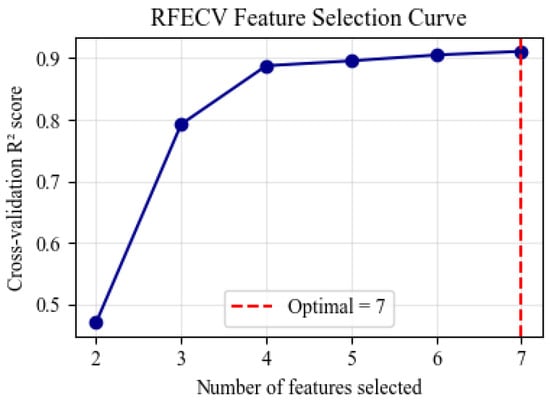
Figure 1. RFECV feature selection curve.

2.2.3. Multicollinearity Analysis

Figure 2 displays the Pearson correlation coefficient heatmap between the seven features (five base features plus two expanded features) and the target variable. Positive values represent positive correlations. Negative values indicate negative correlations. A larger absolute value, denoted by a deeper color, reflects a higher degree of correlation. As observed in Figure 2, the correlation coefficient between K_a(φ) and φ reaches −1.0, indicating a perfect linear correlation. The correlation coefficient between I and Δ/H is 0.78. This also suggests a high degree of collinearity between them. Furthermore, the correlation coefficient between the base features $\gamma$ and φ reaches 0.88. This is attributed to two factors: first, sandy soils with higher unit weights tend to possess lower porosity and tighter particle contact, leading to larger internal friction angles. Second, it may be related to the specific soil properties of the samples within the database.

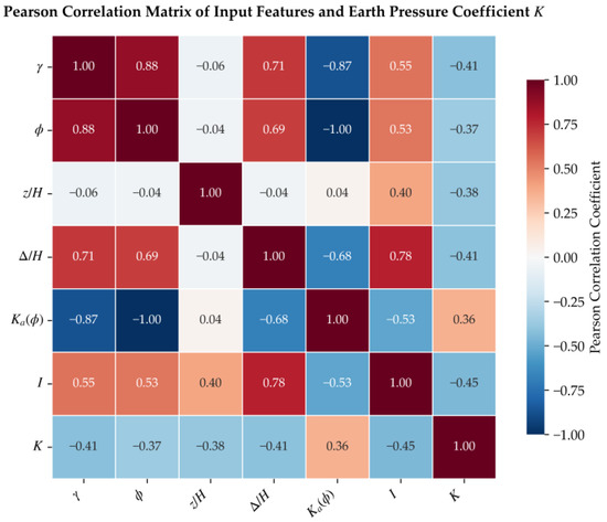
Figure 2. Pearson correlation coefficient heatmap.

This study employs the Variance Inflation Factor (VIF) to analyze the input features. For each independent variable x_i in the model, the VIF is defined as:

$${VIF}_j={\displaystyle \frac{1}{1-R_j^2}}$$

(2)

where $R_j^2$ is the coefficient of determination obtained by regressing x_j as the dependent variable against all other independent variables. When VIF = 1, it indicates no linear correlation between the variable and others, signifying the absence of multicollinearity. When 1 < VIF < 5, the degree of multicollinearity is generally considered mild and acceptable. When VIF > 5, it suggests severe multicollinearity that requires further treatment.

Table 2 presents the results of the VIF analysis. As shown in Table 2, the VIF value for K_a(φ) and φ reaches approximately 2000, indicating extremely severe multicollinearity. Combined with the Pearson correlation coefficient of −1 between K_a(φ) and φ shown in Figure 2, the feature K_a(φ) is excluded while the base feature φ is retained. The six features retained at this stage are $\gamma$, φ, z/H, Δ/H, DM, and I.

Table 2. Feature Collinearity Analysis (VIF Value).

Feature Set	γ	φ	z/H	Δ/H	Ka(φ)	I
Basic features + Ka(φ) + I	6.21	2105.22	1.87	5.00	1990.01	4.67

2.2.4. Comparison of Interpretability Across Feature Sets

Figure 3a,b display the SHAP summary plots (beeswarm) for the six-feature model (base features plus interaction term I) and the five-feature model (base features only), respectively. In the six-feature model (Figure 3a), the interaction term I absorbs the majority of the depth-displacement coupling signals, leading to a significant reduction (approximately by half) in the SHAP value magnitudes for the original parameters z/H and Δ/H. Furthermore, the distribution of their point clouds narrows considerably, and their physical independence is severely undermined.

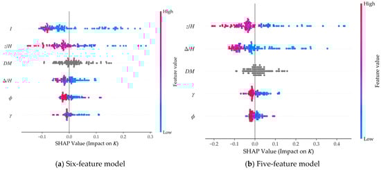
Figure 3. SHAP bee swarm plot. The displacement mode DM is a categorical variable whose values do not imply a numerical magnitude; therefore, its scatter points are displayed in gray.

In contrast, in the five-feature model (Figure 3b), z/H and Δ/H regain their dominant positions. Their contribution magnitudes are substantial, their directions are rational, and their distributions are robust, which aligns closely with the independent driving mechanisms of depth and displacement on active earth pressure in classical soil mechanics. This comparison demonstrates that the collinearity elimination strategy, based on Pearson correlation coefficients and VIF, effectively restores the physical significance and interpretive reliability of key engineering parameters.

Figure 4a,b illustrate the SHAP dependence plots for Δ/H in the six-feature and five-feature models, respectively. In the six-feature model (Figure 4a), the contribution of Δ/H exhibits pronounced wave-like fluctuations and crosses the zero-contribution line multiple times. This behavior contradicts the classical soil mechanics principle that displacement leads to a monotonic reduction in active earth pressure, reflecting severe interference and distortion of the interpretative capacity of the original displacement parameter by the highly collinear interaction term (z/H·Δ/H).

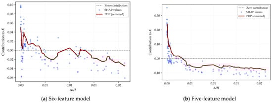
Figure 4. SHAP dependency plot for Δ/H.

In contrast, in the five-feature model (Figure 4b), Δ/H displays a typical L-shaped monotonic downward trend, where the contribution decays rapidly in the small-displacement region before stabilizing. This observation aligns closely with the empirical law in engineering practice, where increasing displacement causes the active earth pressure to gradually converge toward a limit value. This comparison demonstrates that the feature refinement strategy based on collinearity analysis effectively restores a rational marginal contribution pattern for key physical parameters and significantly enhances the physical interpretability of the model.

Unlike Δ/H, the SHAP dependence trends for the other major physical parameters ($\gamma$, z/H, DM, and φ) remain largely consistent across both feature sets. This indicates that the collinearity elimination primarily addresses the interpretative distortion caused by the interaction term, without significantly altering the contribution patterns of other independent physical quantities.

As observed from the curves in Figure 1, the performance improvements of the seven-feature or six-feature models are marginal compared to the five-feature model. Conversely, the inclusion of highly collinear features severely interferes with the SHAP evaluation of fundamental physical quantities. Therefore, this study ultimately determines the five base features listed in Table 1—namely $\gamma$, φ, z/H, Δ/H, and DM—as the optimal model inputs.

2.3. Algorithm Selection

This study selects four representative machine learning algorithms for comparison: Categorical Boosting (CatBoost v1.2.3, Yandex LLC, Moscow, Russia) [38,39,40], Artificial Neural Networks (ANN) [41,42,43], Support Vector Regression (SVR) [44,45], and Random Forest (RF) [46]. These algorithms are representative of different modeling paradigms: SVR and ANN represent traditional algorithms based on kernel functions and neural networks, respectively, while RF and CatBoost represent the Bagging and Boosting approaches within ensemble learning. Notably, since the movement mode in the input features is a categorical variable, CatBoost receives particular attention in this study due to its superior capability in handling categorical features, robust anti-overfitting properties, and rapid inference speed.

This study develops predictive models for each of the four machine learning algorithms mentioned above. These models are implemented using Python (v3.11.7, Python Software Foundation, Wilmington, DE, USA) with the Anaconda environment (Anaconda Inc., Austin, TX, USA), with the Scikit-learn library (v1.2.2, INRIA, Paris, France) used for traditional algorithms. To quantitatively evaluate their predictive accuracy from multiple dimensions, three widely recognized statistical metrics are employed [47]: the Coefficient of Determination (R²), Root Mean Squared Error (RMSE), and Mean Absolute Error (MAE).

The comparison of model performance is presented in Figure 5. Figure 5a shows a grouped bar chart of model performance for various algorithms under default hyperparameters, while Figure 5b illustrates the performance after hyperparameter tuning. As observed in Figure 5a, the ensemble algorithms (RF and CatBoost) demonstrate excellent performance even before hyperparameter tuning, with R² values reaching 0.939 and 0.934, respectively. In contrast, the traditional algorithms (ANN and SVR) yield significantly lower R² values of only 0.542 and 0.738. After hyperparameter tuning, the performance of the ANN and SVR models improves significantly, with R² reaching 0.712 and 0.828, respectively. However, the performance metrics for RF do not show improvement, and those for CatBoost even exhibit a slight decrease.

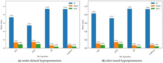
Figure 5. Comparison of model performance across algorithms.

The observation that traditional algorithms (ANN and SVR) experience significant performance gains after hyperparameter tuning, while ensemble algorithms (RF and CatBoost) show limited improvement, is consistent with previous findings [47,48]. Traditional algorithmic models typically assume complex hypothesis spaces, making their performance highly sensitive to hyperparameter configurations. Furthermore, the default hyperparameters of these traditional algorithms often represent a conservative compromise, failing to fully exploit the model’s potential. Zhang et al. [48] noted that the performance of traditional algorithms can be substantially enhanced through tuning, potentially reaching levels comparable to ensemble models.

In contrast, advanced ensemble algorithms such as RF and CatBoost effectively reduce variance and mitigate overfitting by constructing a large number of weak learners and aggregating them through voting or weighted averaging mechanisms. More importantly, the default parameters of ensemble algorithms are typically empirical values that have been extensively optimized by the developer community to perform well across diverse datasets. Consequently, the margin for performance enhancement remains limited even with meticulous hyperparameter searches. This phenomenon suggests that for ensemble models, extensive hyperparameter tuning may not be cost-effective [49], and research efforts should be prioritized toward feature engineering and data quality.

The observed phenomenon that the performance of CatBoost slightly declines after hyperparameter tuning can be attributed to the “CV-Test Generalization Gap,” where cross-validation (CV) optimization succeeds, yet the actual deployment performance decreases. The reasons for this gap can be explained from three perspectives. First, hyperparameter search algorithms may over-explore local optimal solutions based on CV metrics; these solutions are highly adapted to specific data partitioning methods but fail to capture universal underlying patterns. Second, when the hyperparameter search space is too large or mismatches the model complexity, the optimization process tends to focus on noise rather than the signal within the CV set. Third, although this study employs equal-frequency stratified sampling to ensure balance, undetected distribution shifts between the training and test sets can cause the optimization process—if overly targeted at the CV set—to amplify these offsets. This serves as a warning that one-sided pursuit of maximizing CV metrics during the optimization process carries a risk of overfitting.

Figure 5 shows that among the four algorithms (CatBoost, RF, SVR, and ANN), the RF model exhibits the best performance metrics. However, since the input features in this study include the categorical variable of movement mode, the CatBoost algorithm offers an inherent advantage in its ability to handle categorical features automatically. Furthermore, the performance of the CatBoost model under default hyperparameters is remarkably close to that of RF (for instance, its R² reaches 99.47% of the RF value). Consequently, the subsequent model interpretation and the development of the Graphical User Interface (GUI) program remain based on the CatBoost algorithm with default hyperparameters. This choice ensures the robustness of the physical trends captured by the model.

2.4. Research Framework

The framework of this study is presented in Figure 6 and is detailed as follows:

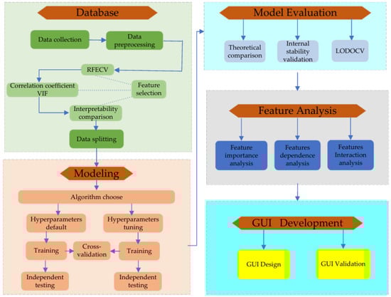
Figure 6. Flowchart of the present study.

(1)

Database Construction: A comprehensive database is established using earth pressure model test data from existing literature. This stage includes data collection, data cleaning, feature normalization, feature encoding, feature selection, and data partitioning. For feature selection, a three-stage refinement strategy is adopted, comprising Recursive Feature Elimination with Cross-Validation (RFECV), collinearity analysis (Pearson correlation and VIF), and a comparison of physical interpretability.

(2)

Algorithm Comparison and Training: Four machine learning algorithms are selected for comparison. Model training is performed using five-fold cross-validation, followed by testing on an independent set. The performance is evaluated via R², RMSE, and MAE. Ultimately, the CatBoost algorithm with default hyperparameters is determined as the primary model for training.

(3)

Model Performance Evaluation: The predictive accuracy of the machine learning model is compared with the calculated results of classical theories. The internal stability of the model is evaluated. Furthermore, the cross-literature generalization is discussed using Leave-One-Dataset-Out Cross-Validation (LODOCV).

(4)

Model Interpretation: SHAP (v0.47.2, University of Washington, Seattle, WA, USA) is utilized for feature importance analysis, dependence plot analysis, and key feature interaction analysis. This enables a visual description and physical interpretation of the relationship between influencing factors and earth pressure.

(5)

GUI Development: A Graphical User Interface (GUI) program is developed. By inputting the wall height, backfill unit weight, internal friction angle, and specific depth, users can rapidly obtain the evolution curves of the earth pressure coefficient for different movement modes as displacement increases. This provides a valuable reference for the stability assessment of retaining walls.

3. Model Performance Evaluation

3.1. Comparison with Classical Theoretical Calculations

In this study, the CatBoost algorithm is trained on the refined feature set using default hyperparameters. The model performance is evaluated on an independent test set and is compared with the earth pressure coefficients calculated using Coulomb’s theory; the comparison results are presented in Figure 7. Since the source literature of the dataset does not provide the wall-soil friction angle, a value of 0.5 times the internal friction angle of the backfill is adopted for the Coulomb theoretical calculations.

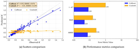
Figure 7. Comparison of predicted active earth pressure coefficients (K). In (a), the gray line represents a perfect match between the predicted and observed values of K.

As observed from Figure 7a, the scatter points predicted by the machine learning (ML) model cluster closely around the 45° identity line with a narrow distribution width, reflecting the high predictive accuracy of the ML model. In contrast, the points calculated using Coulomb’s theory are distributed horizontally within the range of 0.2 to 0.3. Aside from an intersection with the 45° line at the lower end (around 0.2), the remaining points deviate significantly from the identity line. This indicates a substantial discrepancy between the results calculated by Coulomb’s theory and the experimental observations; furthermore, this discrepancy widens as the state approaches the at-rest condition. Figure 7b further provides a quantitative comparison of the two approaches using three metrics (1—R², MAE, and RMSE). The results demonstrate that the ML model performs significantly better than classical theory—which can only provide a single fixed value—in describing the transition zones of non-limit states.

3.2. Internal Stability Assessment

To verify the internal stability of the model, five-fold cross-validation is employed. The entire dataset is randomly divided into five folds. In each iteration, one fold is used as the validation set, while the remaining four folds are used as the training set. Figure 8 shows the comparison between the predicted values and the true values for the validation set samples. As can be seen from Figure 7, the predicted active earth pressure coefficients (K) are symmetrically and densely distributed along the identity line (y = x). Although the data used in this model come from multi-source geotechnical engineering experiments and inherently contain randomness, the model achieves a consistently high R² (average 0.8829) with minimal outliers. This tight clustering demonstrates the model’s robust capability in internalizing the non-linear mapping between features and soil pressure responses.

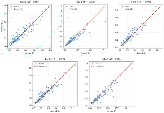
Figure 8. Five-fold cross-validation predicted versus actual value.

Figure 9 displays the residual scatter plot for all samples. As observed from Figure 9, although the data originate from four distinct experimental sources (Refs. [16,18,19,37]), the majority of the colored scatter points—representing different literature sources—are distributed closely and randomly around the central red dashed line (the zero-residual line). The residuals do not exhibit any significant “stratification” or “clustering” based on color. This indicates that the CatBoost model, by learning physical features such as movement modes and internal friction angles, successfully offsets the systematic errors introduced by different laboratory equipment and environments.

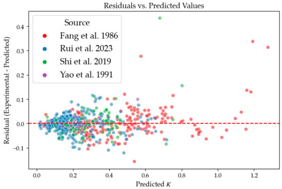
Figure 9. Residuals versus predicted values [16,18,19,20].

Notably, in the region where K > 0.8 (predominantly the red points from Ref. [16]), the residual fluctuations increase. This is likely due to the fact that the at-rest earth pressure state during the infinitesimal displacement stage is heavily influenced by latent factors such as backfill compaction, which carries inherent physical uncertainty.

Figure 10 presents the error distribution histogram for all samples. As observed from Figure 10, the error distribution exhibits the characteristics of a normal distribution, with a mean extremely close to zero (μ = 0.0013) and a small standard deviation (σ = 0.0472). This indicates that approximately 95% of the prediction errors are controlled within a range of about 0.09 (corresponding to 2σ). According to Gaussian error distribution theory, this confirms that the present model is a reliable unbiased estimator, whose prediction errors are random rather than systematic.

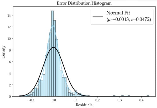
Figure 10. Error distribution histogram. The blue line denotes the Kernel Density Estimation (KDE) of the data distribution, while the black line represents the theoretical normal distribution curve (μ = −0.0013, σ = 0.0472).

The aforementioned five-fold cross-validation and residual analysis demonstrate that the CatBoost model established in this study displays strong internal robustness and generalization capability across heterogeneous laboratory datasets. It successfully captures the underlying physical mechanisms without being dominated by discrepancies in data sources. These internal validation results lay a solid foundation for the subsequent exploration of earth pressure physical laws.

3.3. Leave-One-Dataset-Out Cross-Validation and Discussion on Cross-Literature Generalization

Considering the heterogeneity across different model tests, this study employs Leave-One-Dataset-Out Cross-Validation (LODOCV) to further verify the cross-literature generalization capability of the model. In this approach, one of the four source publications is reserved as an independent validation set, while the samples from the remaining three publications serve as the training set. This process is repeated four times, such that each dataset is used as the test set once. The results of the LODOCV are presented in Table 3.

Table 3. Leave-One-Document-Out Cross-Validation (LODOCV) evaluation metrics.

Paper of Testing Samples	Number of Training Samples	Number of Testing Samples	RMSE	MAE	R2
Ref. [16]	397	233	0.2376	0.1840	0.2817
Ref. [18]	317	313	0.1432	0.1115	−0.1533
Ref. [19]	555	75	0.1410	0.1071	0.4060
Ref. [37]	621	9	0.0676	0.0584	−0.5033

As is observed from Table 3, the model performance metrics obtained through LODOCV are notably lower. Although the database includes fundamental physical parameters such as φ and γ, the specific experimental environments across different publications—such as model box size effects, variations in friction angles due to wall materials, uniformity of soil density, and anisotropy caused by sample preparation—represent “latent variables” that the model cannot capture. Consequently, while the established model exhibits high accuracy within the training sets, its predictive precision may decrease significantly when applied to entirely unseen literature data.

However, this does not signify model failure. As demonstrated in the subsequent discussions, the model successfully captures the fundamental development laws of earth pressure, such as the monotonic decreasing trend of K with increasing displacement. This proves that the model learns universal mechanical logic rather than over-fitting to specific experimental values. Such heterogeneity is a common pain point in the current field of geotechnical machine learning and may be the primary reason why studies utilizing machine learning for direct earth pressure prediction remain rare. This study quantitatively highlights these challenges through LODOCV and suggests that future research should incorporate a broader range of soil types and field data to enhance generalization, and emphasizes that, under current data constraints, machine learning should prioritize the discovery of physical laws in earth pressure to provide a scientific basis for the rational design of retaining walls.

4. Research on Earth Pressure Mechanisms

4.1. Feature Importance Analysis

Figure 11 presents the feature importance ranking derived using the SHAP framework under the default hyperparameters of the CatBoost model. The horizontal axis corresponds to the mean absolute SHAP value for each input feature, while the vertical axis lists the features in descending order of their contribution to the model output. The numerical label on the right side of each bar indicates its contribution rate. Figure 12 displays the SHAP summary plots in the form of violin plots, where the width reflects the kernel density estimation (KDE) of the SHAP value distribution.

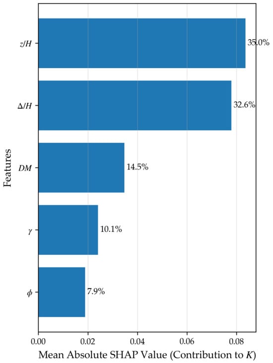
Figure 11. Feature importance ranking plot.

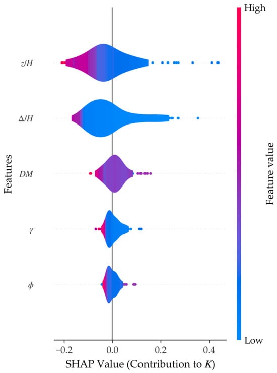
Figure 12. SHAP violin plot.

As shown in Figure 11, relative depth (z/H) is identified as the most influential feature, accounting for 35.0% of the total contribution. In the corresponding violin plot (Figure 12), higher values of z/H are associated with lower (more negative) SHAP values, indicating that samples from greater depths correspond to smaller earth pressure coefficients. From a physical mechanism perspective, this statistical trend captures the nonlinear distribution of earth pressure caused by soil arching effects. As the wall displaces, the uneven movement between soil layers triggers a transfer of stress, making the earth pressure coefficient depth-dependent—a phenomenon that contrasts with the constant coefficient assumption in classical Rankine or Coulomb theories.

Relative displacement (Δ/H) ranks second at 32.6%. The violin plot shows that larger Δ/H values correspond to lower SHAP values, aligning with the transition from an at-rest state toward an active state. Critically, this influence is closely linked to the development of shear bands within the backfill. As Δ/H increases toward a critical threshold, the localized shear strain accumulates to form continuous sliding surfaces. The model’s high sensitivity to Δ/H reflects the physical process where the mobilization of soil shear strength drastically alters the lateral stress path.

The displacement mode (DM) contributes 14.5%. While classical theories often ignore the mode of movement, SHAP analysis confirms its non-negligible role in altering stress distribution and deformation paths. Existing studies [15] have demonstrated that different displacement modes can alter the stress path and displacement path of the soil behind the wall, thereby influencing the magnitude of earth pressure. The interaction between DM and Δ/H later in this paper indicates that the “physical essence” of earth pressure is not merely a function of soil constants, but a result of the kinematic constraints imposed by the retaining structure.

The soil unit weight (γ) ranks fourth (10.1%). Interestingly, higher unit weight corresponds to lower SHAP values in this model. This may be explained by soil compaction: for dry sandy soils, a higher unit density often indicates denser packing and stronger particle interlocking, which indirectly enhances the shear resistance.

The internal friction angle (φ) ranks last with a contribution of 7.9%. While φ is a primary governing parameter in classical theories, its lower relative importance in this specific SHAP analysis should be interpreted with caution. This outcome does not necessarily imply a fundamental contradiction with physical laws, but rather reflects the following:

(a)

The influence of φ may be partially “absorbed” by γ due to the strong physical correlation between soil density and friction angle in the dataset.

(b)

In the presence of significant wall movement, the variability in the earth pressure coefficient is more sensitively captured by displacement-related parameters (Δ/H and DM) than by the inherent soil strength parameters.

(c)

The statistical importance is inherently tied to the parameter ranges within the training data of this model.

4.2. Nonlinear Analysis of Earth Pressure Mechanism

To examine more clearly how the earth pressure coefficient varies with different input features, SHAP dependence plots are presented in Figure 13. In these plots, the vertical axis quantifies the feature’s statistical contribution to the model output (K), illustrating the nonlinear relationship captured by the CatBoost model.

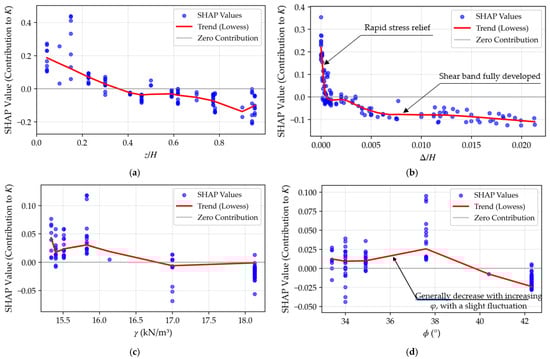
Figure 13. SHAP dependence plots for individual features: (a) Relative depth z/H; (b) Relative displacement Δ/H; (c) Soil unit weight γ(kN/m³); (d) Internal friction angle φ (°). Blue dots represent test set samples; red lines indicate the Lowess-smoothed trend. Vertical axes denote the SHAP value, representing the contribution to the predicted coefficient K.

As shown in Figure 13a, smaller z/H values correspond to larger SHAP values, indicating that shallower soil depths contribute to a higher predicted earth pressure coefficient K. This statistical trend is consistent with the physical phenomenon of soil arching. In real retaining structures, the relative movement between the wall and the backfill triggers a transfer of active pressure from more yielding zones to less yielding ones. The model successfully captures this nonlinear vertical distribution, which mirrors experimental observations by Fang et al. [16], Zhou et al. [17], Singh et al. [24], and Gramegna et al. [50]. Rather than contradicting classical theory, these results provide a data-driven refinement of the depth-invariant assumption in Rankine or Coulomb formulations by accounting for internal stress redistribution.

Figure 13b reveals that in the initial stage (0 < Δ/H < 0.001), SHAP values decrease sharply with increasing displacement. Beyond this range, the reduction becomes more gradual. This transition reflects the physical essence of the soil’s stress path as it moves from an at-rest state toward an active state. The initial steep drop corresponds to the rapid mobilization of soil shear strength. As displacement approaches a critical threshold (e.g., Δ/H ≈ 0.006 as observed in typical sandy soils), the localized shear strains begin to coalesce into continuous shear bands. Once the failure surface is fully developed, the earth pressure coefficient tends to stabilize. The narrow distribution of scatter points around the dependence curve suggests that Δ/H is a primary kinematic driver with relatively independent influence on the coefficient’s reduction.

Figure 13c indicates that K generally decreases as γ increases. From a mechanical standpoint, this aligns with the effect of soil compaction. Denser packing in sandy soils leads to stronger particle interlocking, which not only enhances shear strength but also makes the soil arching effect more pronounced [16].

In contrast, the dependence curve for the internal friction angle (φ) in Figure 13d shows a nuanced, non-monotonic relationship. Between 33.5° and 38°, the contribution to K increases slightly before exhibiting the expected decreasing trend at higher angles. It is important to distinguish this statistical observation from a fundamental physical contradiction. This non-monotonicity likely stems from feature correlations (e.g., the coupling between φ and γ in the dataset) or sampling bias within specific parameter ranges. While classical theories treat φ as an independent governing constant, the model reflects its complex interaction with other factors under realistic, multifactor-coupled conditions. In engineering practice, however, selecting backfill with a higher φ remains a reliable heuristic for reducing lateral pressure.

4.3. Analysis of Feature Interactions in Earth Pressure

To further elucidate the nonlinear mechanisms of stress redistribution within the backfill, SHAP dependence interaction plots are constructed to examine the statistical coupling between relative displacement (Δ/H) and relative depth (z/H), as well as between Δ/H and displacement mode (DM) (Figure 14). These interaction plots visualize how the model’s sensitivity to one feature is modulated by another, reflecting the complex, multifactor-coupled response of the soil-structure system.

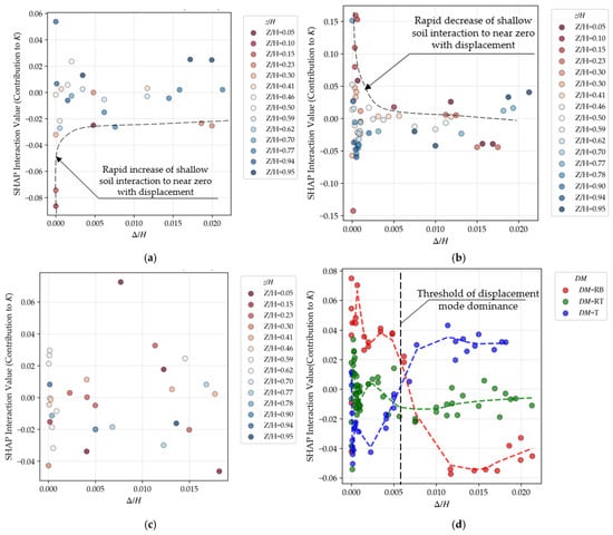
Figure 14. SHAP interaction plots between Δ/H and other features: (a–c) Interaction with z/H under RB, RT, and T modes; (d) Interaction with displacement mode (DM). In (a–c), the redder the scatter point color, the shallower the burial depth; the bluer the scatter point color, the greater the burial depth. The intersection in (d) highlights a mechanical threshold near Δ/H ≈ 0.006: prior to this point, the displacement mode (spatial distribution) governs the stress response; beyond it, the displacement magnitude dominates as the continuous shear band (sliding surface) becomes fully developed.

4.3.1. Interaction Between Relative Displacement (Δ/H) and Relative Depth (z/H)

Figure 14a–c present the interaction effects under the rotation-about-the-base (RB), rotation-about-the-top (RT), and translation (T) modes, respectively. These results provide a data-driven visualization of the spatial non-uniformity in the backfill stress state.

In the RB mode (Figure 14a), SHAP values in the shallow region (low z/H) show negative interaction effects. With increasing Δ/H, these values converge rapidly toward zero, suggesting a quicker transition to the active earth pressure state. Physically, this reflects a stress path where the mobilization of shear strength begins at the wall crown. The large displacement at the top facilitates a complete stress release, while the kinematic constraint at the base delays the relaxation of deep soil layers.

In the RT Mode (Figure 14b), conversely, the shallow zone initially exhibits positive SHAP interaction values. This aligns with the enhanced soil arching effect. The restraint at the wall top forces a stress concentration in the upper backfill, effectively transferring pressure from the yielding lower zones to the constrained top. The model captures the progressive failure of this “soil arch” as displacement increases, eventually leading to a shift toward negative contribution.

In the T Mode (Figure 14c), the absence of a pronounced stratified trend suggests that the variation in earth pressure is primarily governed by the linear increase in overburden stress rather than a displacement gradient.

The aforementioned SHAP analysis of the interaction between Δ/H and z/H confirms that the model remains faithful to classical soil mechanics principles, particularly regarding the spatial non-uniformity of earth pressure. In the RB (Rotation about the Base) mode, the strong negative correlation between Δ/H and z/H at shallow depths highlights the initial rapid stress relaxation at the wall top, which gradually diminishes toward the rigid base. Conversely, the RT (Rotation about the Top) mode presents a complex nonlinear interaction pattern. As displacement occurs, the interaction effect near the ground surface (z/H ≈ 0) is weakened, which represents the model’s manifestation of the soil arching mechanism—a mechanism that offsets the pressure drop typically induced by displacement magnitude.

These findings are validated by the studies of Fang et al. [16] and Rui et al. [18]. Consequently, these interaction plots serve as compelling evidence that the machine learning model successfully learns and incorporates the soil-structure interaction mechanisms that depend on kinematic characteristics.

4.3.2. Interaction Between Relative Displacement (Δ/H) and Displacement Mode (DM)

As illustrated in Figure 14d, the model’s sensitivity to different movement modes evolves significantly with the magnitude of wall displacement. The interaction curves for the three modes exhibit a distinct crossover and convergence at a threshold of approximately Δ/H ≈ 0.006 (within a practical range of 0.005–0.007).

From a soil mechanics perspective, this threshold corresponds to a phased transition in the development of internal shear bands within the backfill. In the pre-threshold stage (Δ/H < 0.006), the spatial distribution of displacement (the movement mode) dominates the stress response. The SHAP interaction values for different modes diverge significantly, indicating that the local mobilization of soil strength makes the stress path highly sensitive to wall rotation or translation. For instance, the RB mode presents higher positive interaction values, reflecting more pronounced local stress relaxation at the top, whereas the RT mode displays stress concentration characteristics dominated by the soil arching effect.

In the post-threshold stage (Δ/H > 0.006), the three curves converge markedly, and the displacement magnitude becomes the primary driving factor as the system approaches a generalized active equilibrium state. This signifies that local shear strains have coalesced to form a fully developed continuous shear band (sliding surface). Once the failure wedge forms, the influence of the specific wall movement mode on the overall earth pressure coefficient diminishes substantially.

This finding suggests that while classical theories (e.g., Rankine or Coulomb) typically assume a translational failure mechanism, they may significantly overestimate pressure under RB conditions or overlook local stress concentrations due to arching under RT conditions during the early stages of displacement. The SHAP interaction analysis thus highlights the necessity of considering mode-dependent stress paths in the refined design of retaining structures.

It should be noted that while these trends align with classical shear band theory, the SHAP results reflect the statistical sensitivity of the model to the training dataset. The observed non-monotonicity in some soil parameters (e.g., φ in Figure 14d) may stem from feature correlations or dataset bias rather than a fundamental contradiction to physical laws. This integrated analysis highlights the necessity of considering mode-dependent stress paths in the refined design of retaining structures.

4.4. Shear Band Evolution and Physical Consistency

The preceding SHAP interaction analysis (Figure 14) demonstrates significant nonlinear coupling between the relative displacement Δ/H, movement mode DM, and relative depth z/H. This section further investigates how the model, through these interaction patterns, captures the progressive evolution of internal shear bands within the backfill and verifies its physical consistency with classical geotechnical principles.

The model’s ability to represent the development from localized strain to a continuous failure surface indicates a high level of physical fidelity. By analyzing the shift in feature influence across different displacement magnitudes, it becomes evident that the model characterizes the transition from a stable soil mass to the formation of a sliding wedge. The alignment with established mechanical theories confirms that the CatBoost model does not merely fit the data points but encapsulates the underlying kinematic mechanisms of soil-structure interaction.

4.4.1. Characterization of Progressive Failure Traits

The SHAP dependence plot for relative displacement Δ/H, shown in Figure 13b, clearly reveals the phased transition characteristics of the earth pressure coefficient K. In the small-displacement stage (when Δ/H is low), the SHAP values decrease rapidly, reflecting the initial mobilization of soil shear strength and a process dominated by elastic deformation. As Δ/H increases, local shear strains gradually concentrate near the potential sliding surface, leading to the formation of a shear band. When Δ/H approaches the critical threshold (approximately 0.006 for typical sandy soils), the SHAP values stabilize, indicating that the continuous sliding surface is fully connected. At this point, the soil enters a stable plastic flow state, and the K value approaches the active earth pressure limit.

This nonlinear behavior aligns closely with the progressive failure mechanism observed in geotechnical engineering [18,51]: the development of the shear band is not instantaneous but expands step-by-step from local yielding to a global sliding surface as displacement accumulates. The model successfully captures this process, proving that it learns not only statistical correlations but also reflects the kinematic essence of soil deformation and strength mobilization.

4.4.2. Synchronization of Soil Arching Effect and Movement Modes

In the Rotation about the Top (RT) mode, the interaction between the soil arching effect and the movement mode (DM) is particularly significant (Figure 14b). As Δ/H increases, the SHAP interaction values for the shallow soil layers in the RT mode shift from positive to negative, which intuitively reflects the formation, development, and eventual collapse of the soil arch. Peng et al. [9] observed through discrete element method (particle flow) simulations that the soil arching effect is most significant in the RT displacement mode compared to other displacement patterns.

Specifically, the wall-top constraint in the RT mode causes stress concentration in the upper backfill, which transfers loads laterally or to lower layers through the soil arching effect. The model assigns high importance to the interaction between z/H and Δ/H, accurately capturing the kinematic constraints of this stress redistribution. Refining the features to five core parameters (z/H, Δ/H, DM, γ, φ) does not diminish the physical depth of the analysis; instead, it eliminates noise interference, allowing the model to focus more effectively on the non-uniform stress field dominated by the soil arching effect.

4.4.3. Convergence with Classical Geotechnical Theories

The evolution patterns of the SHAP analysis curves align closely with Coulomb’s sliding wedge theory and the principles of progressive failure, verifying the physical reliability of this parsimonious model. Unlike black-box models that may rely on physically infeasible feature combinations, the K values predicted by this model adhere to the friction-based yield criteria of granular materials. Specifically, the model correctly reflects the general trend where an increase in φ leads to a decrease in K (notwithstanding slight local non-monotonicity primarily stemming from feature correlations), while emphasizing the dominant role of displacement parameters (Δ/H, DM) in the transition to the active state.

These results indicate that CatBoost effectively learns the primary physical mechanisms of earth pressure development through a data-driven approach. This provides an interpretable basis for the refined design of retaining structures while avoiding the limitations of over-reliance on empirical assumptions.

5. Development and Validation of the GUI Tool

Based on the earth pressure coefficient prediction model established using the CatBoost algorithm with default hyperparameters, a Graphical User Interface (GUI) program is developed for predicting the active earth pressure coefficients of rigid retaining walls. By simply inputting the internal friction angle, unit weight of the sandy backfill, and wall height—while specifying the relative height of the calculation point—the program invokes the pre-trained CatBoost model. It then outputs the evolution curves of the earth pressure coefficient at that specific point across different movement modes as displacement increases. Furthermore, the program provides a direct comparison with classical at-rest earth pressure coefficients and Rankine earth pressure coefficients.

This tool bridges the gap between advanced machine learning algorithms and practical engineering design. It allows users to visualize the non-linear transition from at-rest to active states, which is often oversimplified in traditional calculations. By integrating the movement mode as a key variable, the GUI offers a more nuanced assessment of wall stability under various kinematic conditions.

To verify the reliability of the program, a case study is conducted with φ = 42°, γ = 18 kN/m³, and z/H = 0.5, as shown in Figure 15. As is observed from Figure 15b, the ML model’s prediction curves lie between the at-rest earth pressure coefficient line (K₀) and the Rankine active earth pressure coefficient line (K_a). As displacement increases, the earth pressure transitions from the at-rest state toward the active state.

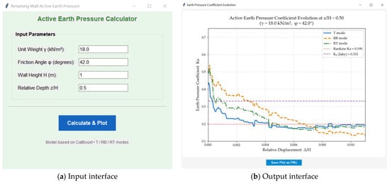
Figure 15. GUI.

Specifically, the curve for the RT mode reaches a plateau at a relative displacement of approximately 0.006, signaling the onset of the active limit state. The RB mode attains this plateau at approximately 0.008, while the T mode does so much earlier, at approximately 0.0042. In the T mode, because the entire wall height moves outward simultaneously, the failure angles of the backfill form almost at once, leading to the earliest achievement of the active limit state. In contrast, the RT mode reaches the limit state later than the T mode due to the more pronounced soil arching effect.

In the RB mode, the displacement at the wall base is zero, providing the strongest constraint on the bottom backfill. The shear zones propagate slowly from the wall top downward. To bring the entire soil wedge into a state of limit equilibrium, the wall top must undergo significant displacement to drive the soil near the base to generate sufficient shear stress. Consequently, this progressive failure process is longer than that in the RT mode.

These results demonstrate that the GUI program successfully captures the physical trends of earth pressure development for various movement modes. It shows that the model provides predictions consistent with mechanical laws across all movement modes and non-limit states. Although its performance is limited by data heterogeneity, it remains superior to classical analytical solutions that cannot account for the influence of displacement.

6. Conclusions and Prospects

This study develops an interpretable framework to extract universal mechanical laws from heterogeneous experimental data. Addressing the limitations of classical earth pressure theories and the significant heterogeneity inherent in various model tests, a predictive model is established using cross-literature experimental data. This model explores the distribution and development patterns of earth pressure for rigid retaining walls with sandy backfill under various movement modes.

A three-stage key feature refinement strategy based on collinearity analysis is proposed and demonstrated. This strategy identifies an optimal feature set consisting of only five fundamental physical parameters, achieving the best balance between predictive accuracy and model interpretability. Building upon the comparison and selection of machine learning algorithms, the CatBoost/SHAP framework is employed to interpret the earth pressure mechanisms during wall displacement. This framework reveals the complex relationships between earth pressure and its various influencing factors. The primary conclusions of this study are as follows:

(1)

A three-stage key feature refinement strategy—comprising “Recursive Feature Elimination, Collinearity Analysis, and Interpretability Comparison”—is proposed. The streamlined feature set constructed through this strategy is utilized for machine learning-based earth pressure coefficient prediction, achieving an optimal balance between predictive accuracy and physical interpretability.

(2)

Leave-One-Dataset-Out Cross-Validation (LODOCV) indicates significant heterogeneity among different retaining wall model test results. This emphasizes that machine learning can establish robust models by integrating cross-literature data to explore the distribution and evolution patterns of earth pressure more comprehensively.

(3)

The CatBoost model, combined with SHAP interpretability analysis, reveals the importance ranking of key features affecting the earth pressure coefficient: relative depth (z/H) makes the highest contribution (35.0%), followed by relative displacement (Δ/H, 32.6%) and movement mode (DM, 14.5%). The study identifies Δ/H ≈ 0.006 as the critical displacement threshold for sandy backfill and suggests that engineering designs use this as a baseline for displacement control. Specifically, before this threshold, focus should be placed on the stress non-uniformity induced by movement modes; after this threshold, the analysis can transition to a limit-state evaluation based primarily on displacement magnitude.

(4)

The patterns identified by SHAP align highly with classical theories, verifying the physical reliability of the parsimonious model. Based on these findings, this study suggests adopting differentiated strategies in refined design: for the RB mode, the safety reserve in the wall-top area should be appropriately increased to address early localized yielding; for the RT mode, structural verification must be strengthened for areas experiencing local stress concentration induced by the soil arching effect. This provides data-driven theoretical support for the design of retaining structures.

(5)

The developed GUI program is capable of providing reasonable predictions for earth pressure coefficients under various working conditions. This tool serves as an auxiliary design means, helping engineers quickly evaluate earth pressure distribution trends under different movement modes and displacement levels during the preliminary design stage, thereby optimizing the stiffness configuration of support structures.

This study breaks through the limitations of classical theories in capturing displacement coupling effects under non-limit states. Its achievements not only deepen the mechanical understanding of earth pressure but also provide specific reference criteria for the displacement-based design (DBD) of retaining structures through quantified displacement thresholds and movement mode sensitivity analysis.

By transitioning from traditional force-based calculations to a more nuanced movement-dependent evaluation, this research offers a robust framework for optimizing the safety and economy of geotechnical infrastructure. The established displacement benchmarks serve as a vital guide for engineers to mitigate risks associated with non-uniform stress distributions and progressive failure in complex urban environments.

Due to the limited number of publications providing complete and detailed experimental records, the dataset in this study is restricted to sandy backfill. Consequently, the model does not incorporate critical design parameters such as wall-soil interface friction, surcharges, and groundwater effects. Furthermore, inherent heterogeneity across different model tests and the discrepancies between idealized laboratory environments and real-world scenarios limit the applicability of the developed model in actual engineering practice. Future research needs to expand the scale and diversity of the dataset, particularly by incorporating more in situ monitoring and field test data to enhance the model’s generalization capability. Meanwhile, it is essential to systematically optimize the selection of input features (such as wall-soil friction angle) and the balance of data distribution. Exploring more interpretable machine learning methods is required to improve the accuracy and reliability of predictions, thereby promoting the widespread application of this approach in geotechnical engineering practice.

References

- Nguyen, T. An Exact Solution of Active Earth Pressure Based on a Statically Admissible Stress Field. Comput. Geotech. 2023, 153, 105066. [Google Scholar] [CrossRef]
- Qian, J.; Zhou, C.; Li, W.; Gu, X.; Qin, Y.; Xie, L. Investigation on the Influencing Factors of K0 of Granular Materials Using Discrete Element Modelling. Appl. Sci. 2022, 12, 2899. [Google Scholar] [CrossRef]
- Ma, K.; Wang, L.; Long, L.; Peng, Y.; He, G. Discrete Element Analysis of Structural Characteristics of Stepped Reinforced Soil Retaining Wall. Geomatics. Nat. Hazards Risk 2020, 11, 1447–1465. [Google Scholar] [CrossRef]
- Yang, M.; Deng, B. Simplified Method for Calculating the Active Earth Pressure on Retaining Walls of Narrow Backfill Width Based on DEM Analysis. Adv. Civ. Eng. 2019, 2019, 1507825. [Google Scholar] [CrossRef]
- Li, T.; Huo, J.; He, P.; Liu, X.; Fang, X. Comprehensive Review of Earth Pressures on Retaining Structure. J. Guilin Univ. Technol. 2017, 37, 94–102. [Google Scholar] [CrossRef]
- Patsevich, A.; El Shamy, U. Discrete-element Method Study of the Seismic Response of Gravity Retaining Walls. Int. J. Geomech. 2020, 20, 04020197. [Google Scholar] [CrossRef]
- Wang, Y.; Mora, P.; Liang, Y. Calibration of Discrete Element Modeling: Scaling Laws and Dimensionless Analysis. Particuology 2022, 62, 55–62. [Google Scholar] [CrossRef]
- Li, Z.; Yang, X. Three-dimensional Active Earth Pressure for Retaining Structures in Soils Subjected to Steady Unsaturated Seepage Effects. Acta Geotech. 2019, 15, 2017–2029. [Google Scholar] [CrossRef]
- Peng, S.; Li, X.; Fan, L. Meso-scale of Soil Arching for Rigid Retaining Wall Active Failure. J. Cent. South Univ. (Sci. Technol.) 2011, 42, 1099–1104. [Google Scholar]
- Handy, R.L. The Arch in Soil Arching. J. Geotech. Eng. 1985, 111, 302–318. [Google Scholar] [CrossRef]
- Liu, Y.; Yu, P. Analysis of Soil Arch and Active Earth Pressure on Translating Rigid Retaining Walls. Rock Soil Mech. 2019, 40, 506–528. [Google Scholar] [CrossRef]
- Lu, W.; Wang, X.; Yang, P.; Cui, L.; Ren, Y.; Jin, K. Analysis of Soil Arching Effect of Active Earth Pressure on Rigid Retaining Wall with Translation Mode. J. Lanzhou Univ. Technol. 2017, 43, 132–136. [Google Scholar] [CrossRef]
- Zhou, Y.; Yang, D. Calculation and Analysis of Active Earth Pressure on Retaining Walls Considering Soil Arching Effects. J. Hohai Univ. (Nat. Sci.) 2016, 44, 149–154. [Google Scholar] [CrossRef]
- Wang, M.; Li, J. New Method for Active Earth Pressure of Rigid Retaining Walls Considering Arching Effect. Chin. J. Geotech. Eng. 2013, 35, 865–870. [Google Scholar] [CrossRef]
- Chang, M. Lateral earth pressures behind rotating walls. Can. Geotech. J. 1997, 34, 498–509. [Google Scholar] [CrossRef]
- Fang, Y.; Ishibashi, I. Static Earth Pressure with Various Wall Movements. J. Geotech. Eng. 1986, 112, 317–333. [Google Scholar] [CrossRef]
- Zhou, Y.; Ren, M. An Experimental Study on Active Earth Pressure behind Rigid Retaining Wall. Chin. J. Geotech. Eng. 1990, 12, 19–26. Available online: https://www.cgejournal.com/cn/article/id/9353 (accessed on 2 January 2026).
- Rui, R.; Jiang, W.; Xu, Y.; Xia, R.; Edo, E.E.; Ding, R. Experimental Study of the Earth Pressure on a Rigid Retaining Wall for Various Patterns of Movements. Chin. J. Rock Mech. Eng. 2023, 42, 1534–1545. [Google Scholar] [CrossRef]
- Shi, W. Model Test and Analytical Research on the Active Earth Pressure Acting on a Rigid Retaining Wall. Master’s Thesis, Chang’an University, Xi’an, China, April 2019. [Google Scholar]
- Qian, Z.-H.; Zou, J.-F.; Tian, J.; Pan, Q.J. Estimations of Active and Passive Earth Thrusts of Non-homogeneous Frictional Soils Using a Discretisation Technique. Comput. Geotech. 2020, 119, 103366. [Google Scholar] [CrossRef]
- Xiao, X.; Li, M.; Wu, H. DEM Simulation of Earth Pressure Exerted on Rigid Retaining Wall Subjected to Confined Soil. Chin. J. Undergr. Space Eng. 2020, 16, 288–294. [Google Scholar] [CrossRef]
- Wan, L.; Zhang, X.; Wang, Y.; Xu, L.; Xu, C. Study on Active Failure and earth Pressure of Cohesionless Soil with Limited Width behind Retaining Wall. J. Civ. Environ. Eng. 2019, 41, 19–26. [Google Scholar] [CrossRef]
- Zhang, H.; Xu, C.; He, Z.; Huang, Z.; He, X. Study of Active Earth Pressure of Finite Soils under Different Retaining Wall Movement Modes Based on Discrete Element Method. Rock Soil Mech. 2022, 43, 257–267. [Google Scholar] [CrossRef]
- Singh, P.; Chakraborty, T.; Mahajan, P. Discrete Element Study of Stresses and Deformation on Gravity Retaining Wall under Static Loading. Granu. Matter 2024, 26, 48. [Google Scholar] [CrossRef]
- Zhang, F.; Yin, M.; Sun, F.; Feng, G.; Sun, J.; Liu, G.; Lin, G.; Li, Q.; Xu, C. Non-Limit Active Earth Pressure Under Different Retaining Wall Displacement Modes Based on Discrete Element Simulation. Sci. Technol. Eng. 2024, 24, 4658–4668. [Google Scholar] [CrossRef]
- Shi, F.; Lu, K.; Yin, Z. Determination of Three-dimensional Passive Slip Surface of Rigid Retaining Walls in Translational Failure Mode and Calculation of Earth Pressures. Rock Soil Mech. 2021, 42, 735–745. [Google Scholar] [CrossRef]
- Chen, H.; Chen, F.; Chen, C.; Lai, D. Failure Mechanism and Active Earth Pressure of Narrow Backfills behind Retaining Structures Rotating about the Base. Int. J. Geomech. 2024, 24, 04024068. [Google Scholar] [CrossRef]
- Harle Shrikant, M.; Wankhade Rajan, L. Machine learning techniques for predictive modelling in geotechnical engineering: A succinct review. Int. J. Geosynth. Ground Eng. 2025, 2, 86. [Google Scholar] [CrossRef]
- Zhang, W.G.; Gou, A.T.C. Multivariate Adaptive Regression Splines for Analysis of Geotechnical Engineering Systems. Comput. Geotech. 2013, 48, 82–95. [Google Scholar] [CrossRef]
- Asgarkhani, N.; Kazemi, F.; Jankowski, R.; Formisano, A. Dynamic ensemble-learning model for seismic risk assessment of masonry infilled steel structures incorporating soil-foundation-structure interaction. Reliab. Eng. Syst. Saf. 2025, 267, 111839. [Google Scholar] [CrossRef]
- Shin, J.; Han, H. Analysis of the Impact on Prediction Models Based on Data Scaling and Data Splitting Methods - For Retaining Walls with Ground Anchors Installed. J. Eng. Geol. 2023, 33, 639–655. [Google Scholar] [CrossRef]
- Hang, L.H.; Dang, F.; Wang, X.; Ding, J.; Gao, J. Calculation and Analysis of Earth Pressure under Limited Displacement Considering Influences of Internal Friction Angle. Chin. J. Geotech. Eng. 2021, 43, 81–86. [Google Scholar] [CrossRef]
- Mishra, P.; Samui, P.; Mahmoudi, E. Probabilistic Design of Retaining Wall Using Machine Learning Methods. Appl. Sci. 2021, 11, 5411. [Google Scholar] [CrossRef]
- Aydın, Y.; Bekdaş, G.; Nigdeli, S. Dimensioning of the Retaining Wall Using Linear Regression, Ridge Regression and Lasso Regresion. In Proceedings of the Conference on New Technologies, Development and Application VIII (NT-2025), Sarajevo, Bosnia and Herzegovina, 26–28 June 2025; Springer: Cham, Switzerland, 2025. [Google Scholar] [CrossRef]
- Attache, S.; Sayah, M.; Terrissa, L.S.; Zerhouni, N. Predicting Passive Earth Pressure Coefficients Using Deep Learning Techniques with Computational Cost and Sensitivity Analysis. Math. Model. Eng. Probl. 2025, 12, 1821–1836. [Google Scholar] [CrossRef]
- Gong, H. Calculation Method and Experimental Verification of Unsaturated Soil Pressure Considering Displacement Effect. Master’s Thesis, Hunan University, Changsha, China, April 2023. [Google Scholar]
- Yao, H.; Wang, H. An Experimental Study on Active Earth Pressure behind Rigid Retaining Wall. Water Transp. Eng. 1991, 9, 18–21. [Google Scholar] [CrossRef]
- Minoru, M.; Satoru, K.; Hiderki, Y. Experimental Study on Earth Pressure of Retaining Wall by Field Tests. Jpn. Soc. Soil Mech. Found. Eng. 1978, 18, 27–41. [Google Scholar] [CrossRef]
- Ke, G.; Meng, Q.; Finley, T.; Wang, T.; Chen, W.; Ma, W.; Ye, Q.; Liu, T.-Y. LightGBM: A highly efficient gradient boosting decision tree. Adv. Neural Inf. Process. Syst. 2017, 30, 3146–3154. Available online: https://proceedings.neurips.cc/paper_files/paper/2017/file/6449f44a102fde848669bdd9eb6b76fa-Paper.pdf (accessed on 2 January 2026).
- Uddin, M.N.; Ye, J.; Deng, B.; Li, L.; Yu, K. Interpretable Machine Learning for Predicting the Strength of 3D Printed Fiber Reinforced Concrete (3DP-FRC). J. Build. Eng. 2023, 72, 106648. [Google Scholar] [CrossRef]
- Rahman, J.; Ahmed, K.S.; Khan, N.I.; Islam, K.; Mangalathu, S. Data-Driven Shear Strength Prediction of Steel Fiber Reinforced Concrete Beams Using Machine Learning Approach. Eng. Struct. 2021, 233, 111743. [Google Scholar] [CrossRef]
- Song, Y.; Wang, F.; Yang, W.; Liang, R.; Zhan, D.; Xiang, M.; Yang, X.; Xu, R.; Lu, M. High-Performance Prediction of Soil Organic Carbon Using Automatic Hyperparameter Optimization Method in the Yellow River Delta of China. Comput. Electron. Agric. 2025, 236, 110490. [Google Scholar] [CrossRef]
- Boser, B.E.; Guyon, I.M.; Vapnik, V.N. A Training Algorithm for Optimal Margin Classifiers. In Proceedings of the Fifth Annual Workshop on Computational Learning Theory; ACM: Pittsburgh, PA, USA, 1992; pp. 144–152. [Google Scholar] [CrossRef]
- Solhmirzaei, R.; Salehi, H.; Kodur, V. Predicting flexural capacity of ultrahigh-performance concrete beams: Machine learning based approach. J. Struct. Eng. 2022, 148, 04022031. [Google Scholar] [CrossRef]
- Yang, Y.; Yang, Y. Hybrid Prediction Method for Wind Speed Combining Ensemble Empirical Mode Decomposition and Bayesian Ridge Regression. IEEE Access 2020, 8, 71206–71218. [Google Scholar] [CrossRef]
- Breiman, L. Random Forests. Mach. Learn. 2001, 45, 5–32. [Google Scholar] [CrossRef]
- Ke, L.; Qiu, M.; Chen, Z.; Zhou, J.; Feng, Z.; Long, J. An Interpretable Machine Learning Model for Predicting of CFRP-Steel Epoxybonded Interface. Compos. Struct. 2023, 326, 117639. [Google Scholar] [CrossRef]
- Zhang, Z.; Zeng, T.; Zeng, Y.; Zhu, P. Explainable Prediction of UHPC Tensile Strength Using Machine Learning with Engineered Features and Multi-Algorithm Comparative Evaluation. Buildings 2025, 15, 3217. [Google Scholar] [CrossRef]
- Arslan, Y.; Lebichot, B.; Kevin Allix, K.; Veiber, L.; Lefebvre, C.; Boytsov, A.; Goujon, A.; Bissyandé, T.; Klein, J. Towards Refined Classifications driven by SHAP Explanations. In Proceedings of the International Cross-Domain Conference for Machine Learning and Knowledge Extraction, Vienna, Austria, 23–26 August 2022; Volume 4, pp. 68–81. [Google Scholar] [CrossRef]
- Gramegna, A.; Giudici, P. SHAP and LIME: An Evaluation of Discriminative Power in Credit Risk. Front. Artif. Intell. 2021, 4, 752558. [Google Scholar] [CrossRef]
- Sun, J. Study on Non-Limit Active Earth Pressure of Retaining Wall Under Different Movement Modes. Master’s Thesis, Zhejiang University, Hangzhou, China, April 2023. [Google Scholar]
Disclaimer/Publisher’s Note: The statements, opinions and data contained in all publications are solely those of the individual author(s) and contributor(s) and not of MDPI and/or the editor(s). MDPI and/or the editor(s) disclaim responsibility for any injury to people or property resulting from any ideas, methods, instructions or products referred to in the content. |
© 2026 by the authors. Licensee MDPI, Basel, Switzerland. This article is an open access article distributed under the terms and conditions of the Creative Commons Attribution (CC BY) license.