Quantifying Vertical Temperature Non-Uniformity for Cold-Formed Steel Structural Fire-Resistant Design

Abstract

The time–temperature curve serves as a fundamental input for calculating structural fire resistance. Accurate acquisition of this curve is essential for designing structures to withstand fire incidents effectively. In this study, fire test temperature variation data were analyzed to develop a comprehensive understanding of the temperature-rise curve, categorized into three primary phases: Confined Fire Phase, Reignition Phase, and Flashover to Fully Developed Fire. To address non-uniform temperature distribution, a temperature reduction coefficient was introduced into the temperature-rise curve formula. This coefficient was derived by fitting experimental temperature data from multiple fire tests, enhancing the formula’s applicability to compartment fires. Furthermore, accounting for non-uniform temperature distribution along compartment height is critical for accurate thermo-mechanical simulations of structural components. To simplify calculations, layer-specific reduction coefficients were proposed: top area (x ≥ 0.7H): 1.0; middle area (x < 0.7H): 0.73; bottom area (x ≤ 0.4H): 0.34. These coefficients, determined through numerical simulations, exhibit broad applicability. In conclusion, precise characterization of temperature-rise curves is vital for structural fire resistance assessment. The proposed methodology and reduction coefficients improve the robustness and generalizability of thermo-mechanical simulations in evaluating structural fire performance.

1. Introduction

Building fires, compared to unpredictable natural disasters such as earthquakes and tsunamis, exhibit a higher probability of occurrence. While their potential for causing loss of life and property is significant, the resulting structural damage can be mitigated through informed design. This controllability underscores the critical importance of incorporating fire resistance into structural engineering. Fire safety engineering is an interdisciplinary field that bridges fire science—concerned with fire development, smoke spread, and occupant evacuation—and structural engineering, which focuses on the response and integrity of buildings under thermal attack. A paramount objective of structural fire design is to ensure sufficient load-bearing capacity during a fire, thereby securing vital time for evacuation. In analytical and design calculations, the complex evolution of a fire is often simplified by applying time–temperature curves as thermal loads on structures. Consequently, determining a realistic and applicable time–temperature curve is fundamental to accurately assessing structural fire performance.

In conventional practice, standard time–temperature curves such as ISO 834 [1], BS 476 [2], and ASTM E119 [3] are employed to represent fire loads. These curves, including those for external [4] and hydrocarbon fires [4], prescribe a uniform temperature rise assumed to occur homogeneously throughout a compartment. However, they represent severe, standardized heating conditions without accounting for specific factors like fire load density, ventilation, or compartment geometry, thus not replicating real fire dynamics.

To better approximate actual fires, parametric models have been developed. Eurocode [4] provides a parametric approach based on the Swedish curve [5], integrating factors such as fire load and opening characteristics. Similarly, ASCE [6] and researchers like Ma Zhongcheng [7] have proposed models derived from experimental statistics. Barnett [8,9,10] introduced the BFD curve, defined by a single equation encompassing both growth and decay phases. While these parametric curves offer improved realism, they typically retain the assumption of a uniform temperature distribution within the fire compartment.

In reality, fires exhibit significant spatial temperature variations, both vertically and horizontally. Fire science models, such as the Two-Zone Model and computational fluid dynamics (CFD)-based Field Models (e.g., NIST’s FDS [11]), can predict this non-uniformity. These tools have been validated for enclosed spaces [12] and even integrated with finite element software for coupled thermo-structural analysis [13,14,15,16]. However, their computational complexity limits routine application in structural design, which often prioritizes vertical temperature gradients due to their critical influence on failure mechanisms. For instance, Shahbazian [17] demonstrated that modeling vertical temperature distribution in distinct zones yielded results closely aligned with experimental tests on walls.

Therefore, a discernible gap exists between advanced, spatially resolved fire models and the practical needs of structural fire resistance assessment. There is a pressing need for a simplified yet realistic fire model that (1) captures the key temporal stages of a real fire, and (2) explicitly incorporates essential vertical temperature non-uniformity in a form readily applicable for structural analysis.

To address this gap, this study develops a staged time–temperature curve model derived from full-scale fire test data. The model delineates three characteristic phases: Confined Fire, Reignition, and Flashover to Fully Developed Fire. Crucially, it introduces a reduction coefficient to efficiently account for vertical temperature decay. Validated against experimental results, the proposed model demonstrates high fidelity to real fire dynamics and serves as a reliable, practical thermal load input for the thermo-mechanical analysis of structural systems under fire conditions.

2. Compartment Fire Test

2.1. Introduction of Experimental Model

To investigate the temperature-rise curve within confined spaces under actual fire conditions, three single-story cold-formed steel (CFS) houses were specifically designed for experimentation (Figure 1; the construction process and structural configuration are detailed in Reference [18]). Each house measured 7.44 m × 7.44 m with a floor height of 3 m (Figure 1a). The layout comprised four rooms, each measuring 3.6 m × 3.6 m, all equipped with door and window openings. Doors were sized at 2.1 m (height) × 0.9 m (width), while windows measured 1.5 m (height) × 1.5 m (width). One room was designated as the fire compartment (R1), where wood cribs served as the fire load. The remaining rooms (R2–R4) featured fire-rated gypsum board cladding on walls and ceilings. The detailed fire load arrangement is shown in Table 1.

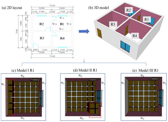
Figure 1. Test model layout and fire load arrangement (unit: mm).

Table 1. Model fire load arrangement.

Model	Fire Load Distribution	Location Description	Simulated Scenario
Model I	Concentrated fire loads	Along the WC-side wall (where the linear density of wood strips is three times that of other areas)	Wall-mounted closets in the red box (Figure 1c)
Model II	Concentrated fire loads	In the corner region (where the density of wood strips is three times that of other areas)	Stacked combustibles in the red box (e.g., curtains, books) (Figure 1d)
Model III	Uniformly distributed fire loads	Across the area (using wood cribs)	Standard distributed fire load (Figure 1e)

The three test models maintained identical layouts with variations in fire load distribution. Following the U.S. standard NFPA 557-2017 [19] “Standard for Determination of Fire Loads for Use in Structural Fire Protection Design”, localized fire loads were implemented where fire load density exceeded 2.57 times the standard room density. Per this standard, fire loads were configured as follows.

The average fire load density across all fire compartments was 935.76 MJ/m².

2.2. Arrangement of Thermocouple Measurement Points in Test Models

K-type thermocouples were installed in the test compartments to monitor real-time temperature changes. The instrumentation layout is detailed in Figure 2, where solid circles denote thermocouple tree locations. Each thermocouple tree contained three measurement points. For example, the 1RT1 tree (Figure 2d) had points labeled: 1RT1-0.5, 1RT1-1.38, 1RT1-2.26. In Model I (Figure 2a), 1RT1-1RT4 monitored the temperature field in fire compartment R1; 1RT5-1RT6 monitored non-fire compartment R2; 1RT7-1RT8 monitored non-fire compartment R3.

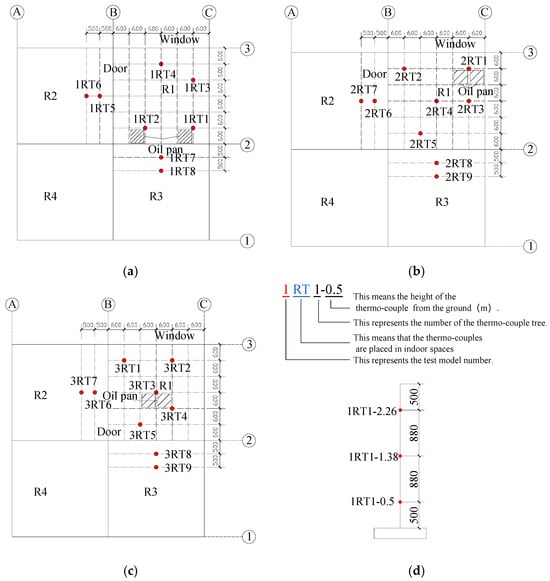
Figure 2. Thermocouple tree layout in test model (mm). (a) Model I. (b) Model II. (c) Model III. (d) 1RT1 thermocouple tree measurement point arrangement.

Thermocouple arrangements for Models II and III are shown in Figure 2b and Figure 2c, respectively. The ignition source location (ignition pan) is indicated in Figure 2a–c.

2.3. Temperature-Rise Curve Analysis of the Test Model

Temperature readings from thermocouples at identical heights were averaged to characterize vertical temperature variations. The temperature-rise curves for all three fire compartment models at different elevations are shown in Figure 3.

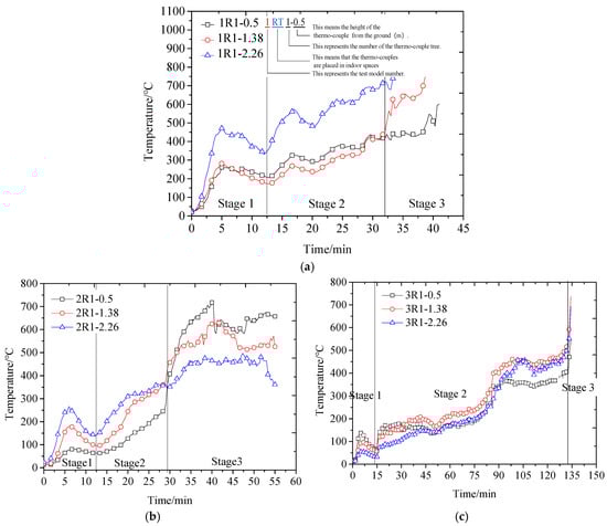
Figure 3. Temperature-rise curve with different heights of room R1. (a) Model I. (b) Model II. (c) Model III.

These curves reveal three distinct fire development stages. The details are provided in Table 2.

Table 2. Detailed description of the three different stages.

Stage	Description
Stage 1 (Confined Fire Phase)	Initial temperature rise followed by decline due to oxygen depletion in the enclosed space, reducing heat release rate and causing temperature drop.
Stage 2 (Reignition Phase)	Temperature spike triggered by fresh air ingress through windows, reigniting wood cribs and inducing secondary temperature rise.
Stage 3 (Flashover to Fully Developed Fire)	Indoor temperatures reach critical levels, causing rapid flame expansion and uncontrolled fire spread.

Comparative analysis of the curves (Figure 3) demonstrates a vertical temperature gradient. During Stages 1–2, significant thermal stratification occurred with higher temperatures at elevated heights. In Stage 3, temperatures converged vertically during the fully developed fire phase.

3. Analysis of Indoor Temperature Rise Throughout Fire Test

3.1. Temperature-Rise Curve Calculation Formula

The indoor temperature-rise curve in fire compartments evolves through three characteristic phases: Confined Fire Phase, Reignition Phase, and Flashover to Fully Developed Fire. Ventilation conditions remain constant during Stages 1 and 3, with openings sealed in Stage 1 and fully open in Stage 3. Stage 2 exhibits variable ventilation due to factors like window glass fracture and high-temperature door failure, making precise quantification challenging.

To accurately characterize the full-process temperature-rise curve in fire compartments, this study proposes a novel time–temperature curve formulation integrating BFD curve [8,9,10]—a parameter-efficient model—with the three characteristic fire development phases. While BFD represents specific ventilation conditions, it effectively depicts Stages 1 and 3 under stable ventilation. For Stage 2, characterized by approximately linear temperature increase, a linear fitting approach was implemented.

Stage 1: Confined Fire Phase

$$T_1=T_0+T_{m1}{e}^{-{\left(\ln t-\ln t_{m1}\right)}^2/Sc}\hspace{1em}t\le t_1$$

(1)

Stage 2: Reignition Phase

$$T_2={T_1}^{\prime }+\left({\displaystyle \frac{500-{T_1}^{\prime }}{t_2-t_1}}\right)\left(t-t_1\right)\hspace{1em}{t}_1<t<t_2$$

(2)

Stage 3: Flashover to Fully Developed Fire

$$T_3={T_2}^{\prime }+\left(T_{m2}-{T_2}^{\prime }\right)e^{-{\left(\ln \left(t-t_2\right)-\ln \left(t_{m2}-t_2\right)\right)}^2/Sc}\hspace{1em}t\ge t_2$$

(3)

where T₁–T₃ represent temperatures at times for Stages 1–3; T₀ denotes the initial ambient temperature; S_C is the shape factor; t_m1 indicates the time to peak temperature in Stage 1; T_m1 is the Stage 1 peak temperature; t₁ defines the window breakage time; t₂ corresponds to flashover occurrence; t_m2 marks the time to peak temperature in Stage 3; and T_m2 is the Stage 3 peak temperature.

3.2. Research on the Non-Uniform Distribution of Temperature with Height

3.2.1. Temperature Reduction Coefficient Calculation Formula

From the temperature-rise curve in the room on fire in the test model (Figure 3), the temperature gradient with height of the temperature-rise curve is evident before flashover (Stages 1 and 2). The temperature of the entire space tends to be the same after flashover (Stage 3); therefore, the temperature change with height is considered for calculating the temperature increase in Stages 1 and 2. Taking the entire temperature-rise curve for the room which is on fire in Test Model II as an example (Figure 4), the temperatures at different heights in Stage 1 first increased and then decreased. The peak temperature was recorded at exactly 7 min. However, there are differences in the peak temperature values (T_m1–2.26 = 274.223 °C, T_m1–1.38 = 153.250 °C, T_m1–0.5 = 101.666 °C, T_m1–2.26 represents the peak temperature of Stage 1 of the time temperature curve at height 2.26), and the peak temperature T_m1 is proportional to the height x above the ground, so a temperature reduction coefficient θ is introduced in Stage 1 to discount the peak temperature T_m1 in order of height above the ground. The difference in the initial temperature along the height direction in Stage 2 (Figure 4) was primarily caused by a gradient in the height direction of the temperature change in Stage 1. At the end of Stage 2, when the fire is about to flashover, the temperature variation tends to be uniform throughout the space, and the difference in temperature along the height direction disappears. To conclude, introducing the temperature reduction coefficient θ in Stage 1 and the discount calculation of the peak temperature T_m1 can realize the non-uniform temperature distribution in the height direction considered in the calculation formula of the temperature-rise curve in Stages 1 and 2.

With the introduction of the temperature reduction coefficient, the equation for Stage 1 of the temperature-rise curve is as follows:

$$T_1=T_0+\left(\theta T_{m1}\right) e^{-{\left(\ln t-\ln t_{m1}\right)}^2/Sc}\hspace{1em}t\le t_1$$

(4)

where the temperature reduction coefficient θ = T_x/T_H, T_x is the peak temperature of Stage 1 of the time–temperature curve at height x from the floor, and T_H is the peak temperature of the Stage 1 of the time temperature curve at height H from the floor. H is the distance from the floor to the ceiling.

In order to obtain a generally applicable temperature reduction coefficient, θ, data on the temperature variation of fire tests recorded in other literature [20,21,22] were acquired. Thirty test sample points were selected, the height ratio x/H and the temperature reduction coefficient θ were listed and fitted, and the fitting results are shown in Figure 5. According to different height ratios x/H, the values of the temperature reduction coefficient θ were divided into three parts: Part 1 was a constant value of 0.338 for x/H ≤ 0.4; in Part 2, the relationship between θ and x/H for 0.4 < x/H < 0.7 was linear; in Part 3, it had a constant value of 1 for x/H ≥ 0.7. The formula (5) for the discount factor θ was derived from the fitting results.

$$\theta =\left\{\begin{array}{cc}0.338& x/\mathrm{H}\le 0.4\\ 1.994{\displaystyle \frac{x}{\mathrm{H}}}-0.4575& 0.4<x/\mathrm{H}<0.7\\ 1& 0.7\le x/\mathrm{H}\end{array}\right.$$

(5)

3.2.2. Verification of Temperature Reduction Coefficient

Based on the temperature distribution of the footprint bedroom fire test in the literature [22], the height ratio x/H and the temperature reduction coefficient θ were calculated and fitted, with the temperature reduction coefficient θ derived from Equation (5), as shown in Figure 6. The data of the test model in [22] were distributed on both sides of the fitted curve, indicating that the temperature reduction coefficient determined using Equation (5) can accurately express the temperature distribution pattern along the height direction when there is a fire in a confined space, with universal applicability.

Figure 4. Temperature-rise curves with different heights of Model II room R1.

Figure 5. Temperature reduction coefficient θ fit.

Figure 6. Comparison of the fitted curve with the fire test.

3.3. Verification of Time–Temperature Curve with Vertical Non-Uniformity

Integrating Equations (1)–(4), the equation for obtaining the time–temperature curve for fire in a confined space considering the non-uniform distribution along the height is as follows:

$$\left\{\begin{array}{ll}{T}_1=T_0+\left(\theta T_{\mathrm{m}}\right) e^{-{\left(\ln t-\ln t_m\right)}^2/Sc}\hfill & t\le t_1\\ T_2={T_1}^{\prime }+\left({\displaystyle \frac{500-{T_1}^{\prime }}{t_2-t_1}}\right)\left(t-t_1\right)\hfill & t_1<t<t_2\\ T_3={T_2}^{\prime }+\left(T_{\mathrm{m}2}-{T_2}^{\prime }\right)e^{-{\left(\ln \left(t-t_2\right)-\ln \left(t_{m2}-t_2\right)\right)}^2/Sc}\hfill & t\ge t_2\end{array}\right.$$

(6)

The time–temperature curve for the process described in Equation (6) was verified based on an actual fire test in a fire-receiving space. The basic information of the model is as follows: the vents of the fire-stricken room are a 1.5 m × 1.5 m (width × length) window and a 0.9 m × 2.1 m (width × length) door. The number of wood strips used as fire load is 1800, each with dimensions of 0.035 m × 0.05 m (section width × length), a height of 0.5 m, and a density of 440 kg/m³. Because the ventilation condition of Stage 1 of the time–temperature curve is such that all vents are closed, the opening factor F_O2 is zero. The shape factor S_C is 4.76 according to S_C = 1/(9.25F_O2 + 0.21). Based on the basic information of the model, the shape factor S_C of the time–temperature curve in Stage 3 is calculated, as shown in Table 3. The shape factor of this stage is 1.206.

Table 3. Calculation of shape coefficient S_C of temperature-rise curve in the third stage.

Parameters	AT1	AV = wVhV	AT2 = AT1 − AV	FV = AVhV	FO2 = FV/AT2	SC = 1/(9.25FO2 + 0.21)
Calculated values	133.374 m2	4.140 m2	129.234 m2	8.694	0.067	1.206

Note: A_T1 is the area inside the fire room, including door and window openings. A_V is the sum of the area of door and window openings in the fire room, h_V is the height of door or window, w_V is the width of door or window, A_T2 is the area inside the fire room excluding the hole, F_V is the ventilation factor, F_O2 is the opening factor, and S_C is the shape factor. The parameter information in the table has been adjusted for accurate representation.

The parameters for calculating each model’s compartment time–temperature curve derive from natural fire test data across three test configurations. Key parameters include the following:

T₀—Measured initial compartment temperature;

t₁—Transition time between Stages 1–2 (first time–temperature curve trough);

T_m1\t_m1—Stage 1 peak temperature and time-to-peak;

t₂—Stage 2–3 transition (defined at 500 °C ignition threshold);

T_m2\t_m2—Stage 3 peak temperature and time-to-peak.

Model III exhibited premature fire extinction without reaching the Stage 3 peak. Given that wood-fueled fires maintain fully developed temperatures ≥800 °C, T_m2 was set to 800 °C at t_m2 = 142.667 min. All parameters are summarized in Table 4.

Table 4. Fire compartment temperature-rise curve parameters.

Model Number	T0 (°C)	t1 (min)	Tm1 (°C)	tm1 (min)	t2 (min)	Tm2 (°C)	tm2 (min)
Model I	23.614	13.000	358.459	5.333	32.333	841.179	40.667
Model II	13.564	12.667	280.649	7.000	31.667	614.325	40.333
Model III	12.498	15.000	141.526	4.333	132.667	800.000	142.667

The measured temperature-rise curves for all three test models at various heights are compared with Equation (6) predictions (Figure 7, Figure 8 and Figure 9). Calculated curves exhibit consistent trends with experimental data. Key observations are shown in Table 5.

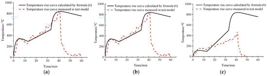
Figure 7. Comparison of the measured temperature-rise curves and Equation (6) for model I. (a) At a height of 2.26 m. (b) At a height of 1.38 m. (c) At a height of 0.5 m.

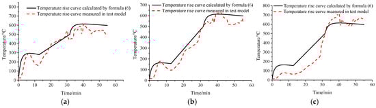
Figure 8. Comparison of the measured temperature-rise curves and Equation (6) for model II. (a) At a height of 2.26 m. (b) At a height of 1.38 m. (c) At a height of 0.5 m.

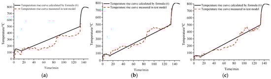
Figure 9. Comparison of the measured temperature-rise curves and Equation (6) for model III. (a) At a height of 2.26 m. (b) At a height of 1.38 m. (c) At a height of 0.5 m.

Table 5. Observation description of models.

Model	Observation Description
Model I	Strong agreement in Stages 1–2; late Stage 3 deviations due to artificial extinguishment causing rapid temperature decline (Figure 7).
Model II	Close alignment between calculated and measured curves at all elevations (Figure 8).
Model III	Experimental curves match Equation (6) predictions at all heights. The predefined 800 °C peak temperature (for prematurely extinguished fires) results in higher calculated values versus measurements (Figure 9).

4. Application of the Time–Temperature Curve Calculation Formula

The time–temperature curve for confined compartments serves as the thermal load for assessing structural member and system responses under fire exposure. Equation (6), developed in this study, provides the primary time–temperature curve for structural fire resistance calculations. Using Wall W_D from Test Model II (Figure 1d) as an exemplar, the thermo-mechanical coupling simulation procedure implementing Equation (6) comprises three essential steps. First, derive the compartment time–temperature curve via Equation (6) and apply it as the thermal boundary condition to the heat transfer model of the cold-formed steel composite wall. Second, compute temperature distributions across the wall section. Finally, map nodal temperatures to the mechanical model for thermo-mechanical analysis to determine fire-induced responses including failure modes and fire resistance time.

Wall W_D (cross-section detailed in Figure 10) incorporates C140 steel studs (2.76 m height), U140 tracks, and a 0.9 m × 2.1 m doorway. Single-layer fire-rated gypsum boards clad both sides, fastened to studs with self-tapping screws at 300 mm spacing. A uniformly distributed vertical load of 2 kN/m² transfers through the header beam to all wall studs. Stud S1 was selected as the control specimen for thermo-mechanical simulation.

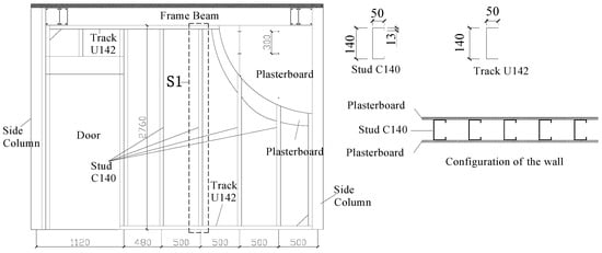
Figure 10. Detailed construction of Wall W_D (mm).

4.1. Temperature Load

4.1.1. Temperature Non-Uniform Distribution Area Division

Equation (5) defines the reduction coefficient θ, partitioning studs vertically into three areas: top, middle, and bottom. The top and bottom areas maintain constant reduction coefficients, while the middle area exhibits linearly varying coefficients.

To evaluate height-dependent temperature non-uniformity effects on cold-formed steel composite wall failure modes, three comparative conditions with distinct vertical temperature gradients were established (Figure 11 and Table 6):

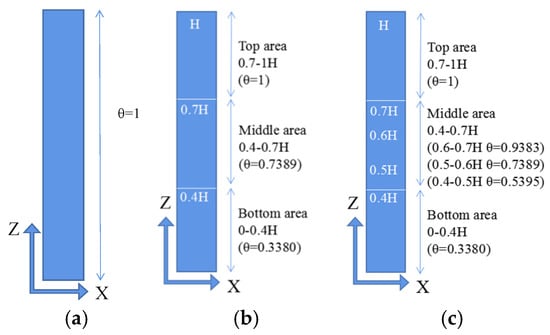
Figure 11. Temperature distribution area division of numerical simulation model. (a) Condition I. (b) Condition II. (c) Condition III.

Table 6. Temperature distribution description of three conditions.

Condition	Temperature Distribution Description
Condition I	Uniform temperature distribution (Figure 11a)
Condition II	Three-area division with middle zone coefficient θ = 0.73 at x = 0.5H (Figure 11b)
Condition III	Top and bottom coefficients matching Condition II, with the middle area subdivided into (0.4H–0.5H), (0.5H–0.6H), and (0.5H–0.6H) to represent internal thermal gradients (Figure 11c)

4.1.2. Time–Temperature Curve

The time–temperature curves of the model at different heights are calculated using Equation (6), as shown in Figure 12, and the above temperature-rise curves are applied as temperature loads to the numerically simulated heat transfer model. The heating regimes for the three models are as follows: Model I assumes a uniform temperature increase along the stud height per Figure 12a. Model II incorporates three distinct areas, each following a specific heating curve from Figure 12b. Model III applies the heating curve from Figure 12c to its top and bottom areas, whereas its middle area (spanning 0.4H to 0.7H) is divided into three sub-areas (0.4–0.5H, 0.5–0.6H, 0.6–0.7H), each with an independent heating profile.

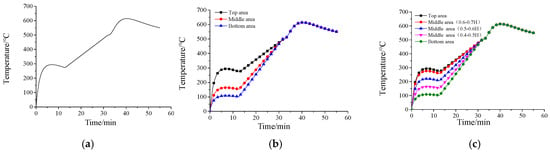
Figure 12. Time–temperature curves of numerical simulation model. (a) Condition I. (b) Condition II. (c) Condition III.

4.2. Numerical Simulation Calculation Model

Cold-formed steel walls are constructed by connecting steel framing members to sheathing panels using self-tapping screws. This construction method introduces multiple types of connections and contacts, such as the following: (1) connections between self-tapping screws and wall panels; (2) connections between self-tapping screws and cold-formed steel members; (3) contact between the track web and the end of studs; (4) contact between the stud flange and the track flange.

Under fire conditions, the mechanical behavior of all these connections exhibits non-linear variation with temperature. If a detailed numerical model reflecting the actual construction were established, the thermo-mechanical coupled simulation would likely face convergence difficulties due to the complex contact interactions. Therefore, simplified approaches for various connections and contacts have been proposed for different wall configurations [23,24].

The numerical simulation follows a sequentially coupled thermal-stress procedure: a heat transfer analysis is first performed, and the resulting nodal temperatures are imported into a mechanical model for structural analysis. In the mechanical model, a single stud may be used to represent the wall behavior. The simplifications in the heat transfer model are described in Section 4.2.1, and those in the mechanical model are introduced in Section 4.2.2. Section 4.2.3 outlines the basic modeling assumptions adopted in this study.

4.2.1. Heat Transfer Model

The heat transfer model shown in Figure 13 [25] was used for the calculation, considering both stud heat conduction and cavity radiation to obtain temperature distribution in the stud cross-section, which was then applied to the mechanical model for the numerical simulation of thermal coupling. The black body heat radiation coefficient in the heat transfer model is 5.67 × 10⁻⁸ W/(m²·k⁴). In this study, a plasterboard is set at 600 °C [26,27,28] shedding; when the temperature reaches 600 °C on the fireside, its thermal insulation is not considered.

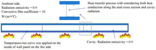
Figure 13. Heat transfer model of cold-formed steel composite wall.

4.2.2. Simplified Thermo-Mechanical Model

The lining panels carry no vertical load in cold-formed steel composite walls. Consequently, the simplified thermo-mechanical model excludes wall panel elements during coupling analysis while accounting for their thermal insulation effect and stud constraint [23]. Boundary conditions in the finite element model are shown in Figure 14:

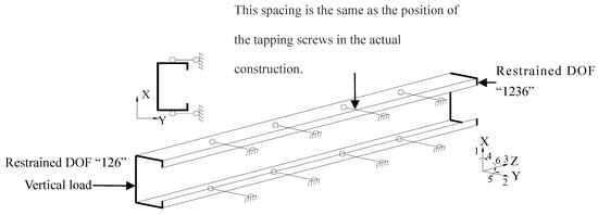
Figure 14. Simplified model of cold-formed steel composite wall.

Wall panel constraints restrain weak-axis bending and torsional deformation (2 DOF constrained);

Plasterboard constraints release upon high-temperature detachment (600 °C critical temperature);

Inter-stud axial springs simulate floor system restraint against thermal expansion, with stiffness calculated per the literature [24];

Applied vertical load: 8.24 kN.

4.2.3. Element Type and Mesh

The numerical model employs S4R shell elements with a mesh size of 5 × 5 cm. The S4R element is a four4-node curved general-purpose shell suitable for both thin and thick shell structures. It uses reduced integration with hourglass control and allows for finite membrane strains. Compared with the standard S4 element, the S4R provides identical accuracy while requiring less storage and offering sufficient degrees of freedom to capture both local and global buckling behavior in cold-formed steel members. Residual stresses, cold-forming effects, and initial geometric imperfections are not considered in the model.

4.3. Material Parameters

4.3.1. High-Temperature Material Properties of Steel

Q345 steel (nominal ambient-temperature yield strength: 345 Mpa) was employed in the cold-formed steel composite walls. The material’s high-temperature degraded properties are presented in Figure 15. Steel’s thermo-physical properties are detailed in Table 7.

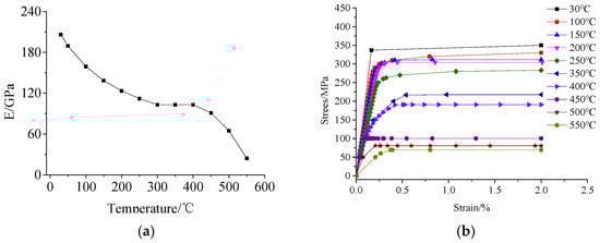
Figure 15. High-temperature material properties of steel. (a) Modulus of elasticity of Q345 steel. (b) Stress–strain curve of Q345 steel.

Table 7. Thermo-physical parameters of Q345 steel.

Temperature (°C)	Thermal Conductivity (W/m∙K)	Specific Heat (J/(kg∙°C))	Coefficient of Thermal Expansion (°C−1)
20	53.33	440.00	7.79 × 10−6
100	50.67	492.62	7.93 × 10−6
200	47.34	549.76	8.16 × 10−6
300	44.01	609.74	9.09 × 10−6
400	40.68	685.88	1.08 × 10−5
500	37.35	791.50	1.36 × 10−5
600	34.02	675.43	1.71 × 10−5

4.3.2. High-Temperature Material Performance of Plasterboard

The density, specific heat, and heat transfer coefficient of the plasterboard varied with the temperature, and the specific values are listed in Table 8.

Table 8. Thermo-physical properties of plasterboard.

Temperature (°C)	Thermal Conductivity (W/(m·K))	Temperature (°C)	Density (kg/m3)	Temperature (°C)	Specific Heat (J/(kg·K))
25	0.3405	0	680	20	1000
80	0.2809	100	680	85	985
160	0.1556	140	564	130	22,010
220	0.1277	600	564	160	1000
300	0.1243	700	544	600	1000
400	0.1589	800	544	660	3000
500	0.2276	1200	544	700	1000
670	0.2851
720	0.3395
800	0.3895
900	0.4453

4.4. Comparison of Numerical Simulation Results with Experiments

4.4.1. Cold-Flange Temperature of Stud

The heat transfer model shown in Figure 13 was used to calculate the temperature field. A comparison between the measured and calculated values of the heat transfer model for the cold-flange temperature of the wall stud is shown in Figure 16. The trends of the measured and calculated values of the heat transfer model are the same. The difference in the temperature values is small, which indicates that the heat transfer model is accurate and provides an assurance of the correctness of the thermal coupling calculation.

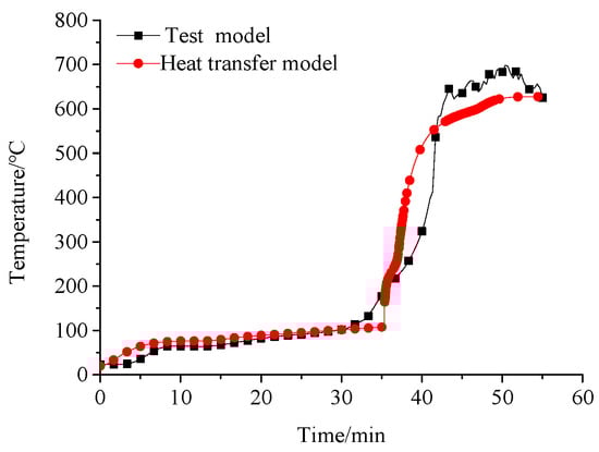
Figure 16. Comparison of test model and heat transfer simulation model of Wall W_D.

4.4.2. Failure Mode

The failure modes of the numerical simulation model and test wall under three working conditions (Figure 11) were compared using fire compartment W_D from Test Model II. Wall W_D’s fire-induced failure modes are shown in Figure 17. All three studs (S1–S3) exhibited the following: bending deformation (X-axis); torsional deformation (Z-axis); local buckling of fire-exposed flanges with deformations concentrated in upper column regions.

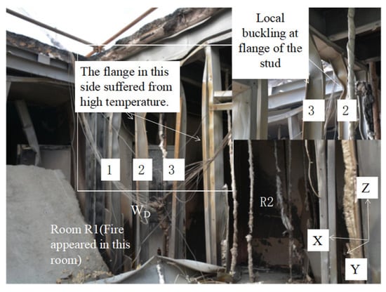
Figure 17. Failure mode of Wall W_D in Test Model II.

This failure mechanism originates from two fire-phase effects:

(1)

Early fire stage: One-sided fire exposure creates cross-sectional temperature gradients, inducing fireside bending deformation under wallboard restraint.

(2)

Late fire stage: Plasterboard board detachment eliminates restraint, triggering torsional buckling.

(3)

Vertical temperature non-uniformity further localized deformations: upper-region boards detached earliest due to higher temperatures, middle boards followed, while lower boards remained intact. Consequently, deformations were concentrated primarily in middle–upper column zones.

The failure modes in the numerical simulation model are shown in Figure 18. Under Condition I (uniform vertical temperature), studs undergo fireside bending deformation (X-axis) before plasterboard detachment. Post-detachment, studs exhibit combined Y-axis bending and Z-axis torsional deformation with local web/flange buckling at both ends. The resultant failure mode—global bending–torsional deformation (Figure 18a)—matches single-layer cladding failure observed in furnace tests.

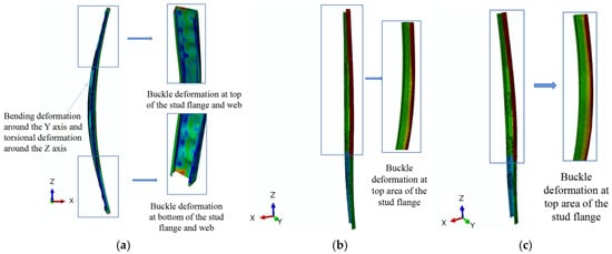
Figure 18. Failure mode of Wall W_D in numerical simulation. (a) Condition I. (b) Condition II. (c) Condition III.

Conditions II and III initially demonstrate identical deformation patterns to Condition I. During later fire stages following gypsum board detachment, torsional deformation superimposes on fireside bending. Deformations concentrate predominantly in middle–upper regions (Figure 18b,c).

Compared with physical tests, Conditions II and III with height-dependent temperature loads replicate actual cold-formed steel wall failure modes and locations. This confirms that vertically non-uniform thermal loading better approximates real fire scenarios. Given identical failure modes and minimal deformation location differences between Conditions II and III, the middle-layer reduction coefficient θ may be simplified per Condition II methodology when applying Equation (6) for thermal load determination.

4.4.3. Fire Resistance Time

The fire resistance time of structural components is governed by three criteria: integrity loss, insulation failure, and load capacity failure. For single-layer gypsum board-clad walls, panel detachment frequently precipitates wall failure due to compromised integrity and insulation. In Test Model II, a single-layer fire-rated gypsum board interior wall underwent integrity verification via ISO 834-compliant cotton pad and gap gauge tests. Limited visibility from smoke obstructed flame observation on the unexposed surface, preventing 10 s duration verification. Consequently, insulation failure was adopted as the wall failure criterion, defined when any unexposed surface point exceeded 180 °C above initial temperature. This yielded a 37 min fire resistance time for Wall W_D.

Load capacity failure occurred later, evidenced by the 600 °C stud flange temperature at 41.33 min. Thus, load-capacity-based fire resistance time was less than 41.33 min. For numerical model comparison, the simulated load capacity failure time was set at 41.33 min.

Numerical simulations require sequential computation: first determining wall cross-section temperature distributions, then executing thermo-mechanical coupling analysis. Insulation failure is temperature-dependent; thus, its occurrence is evaluated using identical criteria to physical tests based on the heat transfer model’s temperature field. Load capacity failure is determined by cross-sectional load reduction in the thermo-mechanical simulation.

Simulation results across the three conditions reveal that load capacity failure times exceed insulation failure times (Table 9), indicating single-layer gypsum board walls fail sequentially—insulation loss precedes load capacity loss—which is consistent with Test Model II’s Wall W_D behavior.

Table 9. Comparison of fire resistance times between the test model and the numerical simulation model.

Disruption Guidelines	Fire Resistance Time (Minutes)			Error (%)
	Numerical Simulation Calculation Model		Test Model
Loss of insulation	Heat transfer model	35.55	37.00	3.92
Loss of carrying capacity	Working condition I	46.60	41.33	12.75
	Working condition II	40.67		1.60
	Working condition III	40.70		1.52

Fire resistance time comparisons (Table 9) demonstrate that Condition I yields longer durations than Conditions II–III, with significant deviation from experimental measurements. This discrepancy confirms Condition I’s thermal load substantially differs from actual fire exposure, necessitating vertical temperature non-uniformity consideration in structural fire design. The minimal 18 s difference between Conditions II and III validates Condition II’s simplified midstory reduction coefficient as representative of real-fire temperature distributions.

5. Conclusions

This study proposes a confined-space time–temperature curve formula derived from spatial temperature field analysis in full-scale fire tests. A reduction coefficient was incorporated to address vertical temperature inhomogeneity. The resulting thermal load was applied to thermo-mechanical simulations of cold-formed steel composite walls, with computational results compared against experimental data. Key conclusions emerge from this work.

(1)

Fire test recordings demonstrate that confined-space heating curves evolve through three characteristic phases: initial confined combustion with temperature rise/decline due to oxygen depletion, subsequent reignition triggered by air ingress, and final flashover to fully developed fire. Significant vertical temperature non-uniformity persists throughout these stages. The staged heating curve formulation integrates principles from Barnett’s BFD curve, enhanced by a height-dependent reduction coefficient. Calibrated against multi-source fire test data, this coefficient exhibits broad applicability to confined fires. The comprehensive formula accounts for both temporal development and vertical thermal gradients, demonstrating high accuracy when validated against experimental temperature fields.

(2)

Thermo-mechanical coupled simulations under three vertical temperature distributions were compared with physical tests. Uniform vertical distribution produced mismatched failure modes and a substantial fire resistance time error (12.75%). Conversely, non-uniform distributions yielded congruent failure modes with minimal time errors (1.60% for Case 2; 1.52% for Case 3). These results confirm that height-dependent temperature profiles are essential for accurate component-level simulations.

(3)

Actual confined-space fires exhibit three distinct vertical thermal regions. This study establishes region-specific reduction coefficients: top area (x ≥ 0.7H): 1.0; middle area (x < 0.7H): 0.73; bottom area (x ≤ 0.4H): 0.34. Derived through comparative analysis of simulation scenarios, these universally applicable coefficients enable efficient computation of compartment temperature fields and reliable thermal loading for structural simulations.

References

- ISO 834; Fire Resistance Tests—Elements of Building Construction. International Organization for Standardization: Geneva, Switzerland, 1975.
- Blagojević, M.Đ.; Pešić, D.J. A new curve for temperature-time relationship in compartment fire. Therm. Sci. 2011, 15, 339–352. [Google Scholar] [CrossRef]
- ASTM E119-98; Standard Test Methods for Fire Tests of Building Construction and Materials. American Society for Testing and Materials: West Conshohocken, PA, USA, 1998.
- EN 1991-1-2; CEN Eurocode 1: Actions on Structures—Part 1–2: General Actions—Actions on Structures Exposed to Fire. European Committee for Standardization: Brussels, Belgium, 2002.
- Magnusson, S.E.; Frantzich, H.; Harada, K. Fire safety design based on calculations: Uncertainty analysis and safety verification. Fire Saf. J. 1996, 27, 305–334. [Google Scholar] [CrossRef]
- Lie, T.T. ASCE Manuals and Reports on Engineering Practice No. 78: Structural Fire Protection; American Society of Civil Engineers: New York, NY, USA, 1992. [Google Scholar]
- Ma, Z.; Mäkeläinen, P. Parametric temperature–time curves of medium compartment fires for structural design. Fire Saf. J. 2000, 34, 361–375. [Google Scholar] [CrossRef]
- Barnett, C.R. Replacing international temperature–time curves with BFD curve. Fire Saf. J. 2007, 42, 321–327. [Google Scholar] [CrossRef]
- Barnett, C.R. BFD curve: A new empirical model for fire compartment temperatures. Fire Saf. J. 2002, 37, 437–463. [Google Scholar] [CrossRef]
- Barnett, C.R.; Clifton, G.C. Examples of fire engineering design for steel members, using a standard curve versus a new parametric curve. Fire Mater. 2004, 28, 309–322. [Google Scholar] [CrossRef]
- Wang, L.; Lim, J.; Quintiere, J.G. On the prediction of fire-induced vent flows using FDS. J. Fire Sci. 2012, 30, 110–121. [Google Scholar]
- Zhao, G.; Beji, T.; Merci, B. Application of FDS to under-ventilated enclosure fires with external flaming. Fire Technol. 2016, 52, 2117–2142. [Google Scholar] [CrossRef]
- Manco, M.R.; Vaz, M.A.; Cyrino, J.C.R.; Landesmann, A. Ellipsoidal Solid Flame Model for Structures Under Localized Fire. Fire Technol. 2018, 54, 1505–1532. [Google Scholar] [CrossRef]
- Prieler, R.; Mayrhofer, M.; Eichhorn-Gruber, M.; Hochenauer, C. Development of a numerical approach based on coupled CFD/FEM analysis for virtual fire resistance tests—Part A: Thermal analysis of the gas phase combustion and different test specimens. Fire Mater. 2019, 43, 34–50. [Google Scholar] [CrossRef]
- Silva, J.C.G.; Landesmann, A.; Ribeiro, F.L.B. Fire-thermomechanical interface model for performance-based analysis of structures exposed to fire. Fire Saf. J. 2016, 83, 66–78. [Google Scholar] [CrossRef]
- Feenstra, J.A.; Hofmeyer, H.; van Herpen, R.A.P.; Maljaars, J. Automated two-way coupling of CFD fire simulations to thermomechanical FE analyses at the overall structural level. Fire Saf. J. 2018, 96, 165–175. [Google Scholar] [CrossRef]
- Shahbazian, A.; Wang, Y.C. Calculating the global buckling resistance of thin-walled steel members with uniform and non-uniform elevated temperatures under axial compression. Thin Walled Struct. 2011, 49, 1415–1428. [Google Scholar] [CrossRef]
- Ye, J.H.; Chen, W.W. Experimental study on fire resistance of full-scale cold-formed steel composite shear wall structure under real fire conditions. J. Build. Struct. 2021, 42, 59–71. (In Chinese) [Google Scholar]
- NFPA 557; Standard for Determination of Fire Loads for Use in Structural Fire Protection Design. National Fire Protection Association: Quincy, MA, USA, 2012.
- Tsai, L.C.; Chiu, C.W. Full-scale experimental studies for backdraft using solid materials. Process Saf. Environ. Prot. 2013, 91, 202–212. [Google Scholar] [CrossRef]
- Kolaitis, D.I.; Asimakopoulou, E.K.; Founti, M.A. Fire behaviour of gypsum plasterboard wall assemblies: CFD simulation of a full-scale residential building. Case Stud. Fire Saf. 2017, 7, 23–35. [Google Scholar] [CrossRef]
- Guillaume, E.; Didieux, F.; Thiry, A.; Bensakhria, A.; Bertin, F. Real-scale fire tests of one bedroom apartments with regard to tenability assessment. Fire Saf. J. 2014, 70, 81–97. [Google Scholar] [CrossRef]
- Chen, W.W.; Ye, J.H. Simplified calculation model for load-bearing CFS composite walls under fire conditions. Adv. Struct. Eng. 2020, 23, 1500–1512. [Google Scholar] [CrossRef]
- Chen, W.W.; Ye, J.H. A new simplified calculation model of CFS composite exterior walls under fire conditions. Structures 2019, 22, 53–64. [Google Scholar] [CrossRef]
- Ye, J.H.; Chen, W.W. Simplified Calculation of Fire Resistant Temperature for Cold-formed Steel Load-bearing Composite Walls. Structures 2020, 28, 1661–1674. [Google Scholar] [CrossRef]
- Sultan, M.A. Comparison of gypsum board fall-off in wall and floor assemblies exposed to furnace heat. In Proceedings of the 12th International Conference on Fire Science and Engineering, Interflam 2010, Nottingham, UK, 5–7 July 2010. [Google Scholar]
- Gerlich, J.T.; Collier, P.C.R.; Buchanan, A.H. Design of light steel-framed walls for fire resistance. Fire Mater. 1996, 20, 79–96. [Google Scholar] [CrossRef]
- Gunalan, S.; Mahendran, M. Fire performance of cold-formed steel wall panels and prediction of the fire resistance rating. Fire Saf. J. 2014, 64, 61–80. [Google Scholar] [CrossRef]
Disclaimer/Publisher’s Note: The statements, opinions and data contained in all publications are solely those of the individual author(s) and contributor(s) and not of MDPI and/or the editor(s). MDPI and/or the editor(s) disclaim responsibility for any injury to people or property resulting from any ideas, methods, instructions or products referred to in the content. |
© 2026 by the authors. Licensee MDPI, Basel, Switzerland. This article is an open access article distributed under the terms and conditions of the Creative Commons Attribution (CC BY) license.