From Pixels to Carbon Emissions: Decoding the Relationship Between Street View Images and Neighborhood Carbon Emissions

Abstract

Under the pressing imperative of achieving “dual carbon” goals and advancing urban low-carbon transitions, understanding how neighborhood spatial environments influence carbon emissions has become a critical challenge for enabling refined governance and precise planning in urban carbon reduction. Taking the central urban area of Xining as a case study, this research establishes a high-precision estimation framework by integrating Semantic Segmentation of Street View Images and Point of Interest data. This study employs a Geographically Weighted XGBoost model to capture the spatial non-stationarity of emission drivers, achieving a median R² of 0.819. The results indicate the following: (1) Socioeconomic functional attributes, specifically POI Density and POI Mixture, exert a more dominant influence on carbon emissions than purely visual features. (2) Lane Marking General shows a strong positive correlation by reflecting traffic pressure, Sidewalks exhibit a clear negative correlation by promoting active travel, and Building features display a distinct asymmetric impact, where the driving effect of high density is notably less pronounced than the negative association observed in low-density areas. (3) The development of low-carbon neighborhoods should prioritize optimizing functional mixing and enhancing pedestrian systems to construct resilient and low-carbon urban spaces. This study reveals the non-linear relationship between street visual features and neighborhood carbon emissions, providing an empirical basis and strategic references for neighborhood planning and design oriented toward low-carbon goals, with valuable guidance for practices in urban planning, design, and management.

1. Introduction

Carbon emissions (CEs) derived from energy consumption constitute a primary driver of global warming. This phenomenon precipitates extreme climatic events, including glacial melting, sea-level rise, heat waves, and hurricanes, thereby posing severe threats to global ecosystems [1,2]. As a major contributor to global CEs, China bears significant responsibility in addressing these environmental challenges [3]. To navigate this challenge, China has established a target to reduce carbon dioxide emissions per unit of GDP by over 65% by 2030, relative to 2005 levels [4]. This initiative aims to drive a profound transformation in the national energy structure and urban development patterns. As the pivotal spatial units for achieving these targets and the primary carriers of energy consumption, cities possess internal structures, spatial organizations, and morphological characteristics that exert direct and profound impacts on CEs [5,6]. Existing research generally posits that urban spatial structure influences CEs by shaping resident activities. Specifically, the optimization of road network structures can mitigate traffic-related CEs [7]; mixed-use functional zoning and intensive land utilization help reduce commuting demand [8]; the expansion of urban green spaces and open areas regulates microclimates [9]; and building attributes and density significantly affect energy consumption [10]. Consequently, these studies underscore that accurate identification of spatial features at the neighborhood scale is a prerequisite for formulating effective carbon reduction policies.

The precise quantification of spatial features at the neighborhood scale relies heavily on the support of emerging data and technologies. With the increasing fusion of multi-source data, Street View Images (SVIs) have emerged as a vital data source for characterizing the physical urban environment [11]. Platforms such as Google Street View and Baidu Street View provide high-resolution, continuously updated open data that effectively capture micro-morphological information, including vegetation, sky, buildings, fences, roads, and public facilities [12,13]. These datasets have been widely applied in domains such as urban environmental exposure, street quality assessment, and the inference of socioeconomic indicators [14,15,16]. Previous studies indicate that street view elements extracted via semantic segmentation can, to a certain extent, characterize regional building quality, green coverage, and living environment features, demonstrating a correlation with energy consumption behaviors [17]. For instance, Chen et al. utilized SVIs to extract building facade features, combining these with machine learning models to predict urban taxi CO emissions [18]. Similarly, Shi et al. extracted visual features, such as buildings, trees, and sky, from SVIs to explain variations in residential CEs [19]. Furthermore, Wu et al. employed SVIs to predict atmospheric pollutant levels [20]. Collectively, these empirical works validate the feasibility of employing SVIs and computer vision to infer complex environmental indicators at a fine spatial granularity.

Despite advancements in data technology, obtaining the CEs data relied upon for model construction remains a severe challenge. Currently, CEs measurement methods primarily include top-down methods, bottom-up methods, and satellite observation. Top-down methods typically estimate emissions based on the total energy consumption of large administrative units, such as provinces or cities [21]. While this method is operationally simple and data-accessible, its accuracy depends on carbon emission factors determined by regional energy structures and technological levels; improper factor selection can lead to biased results [22,23]. Some scholars have identified a significant linear relationship between nighttime light data and CEs, utilizing this data for spatial estimation [24,25,26]. By leveraging the accessibility, global coverage, and temporal continuity of nighttime light data, this approach compensates for the limitations of traditional statistical data regarding spatiotemporal resolution and update frequency. Conversely, bottom-up methods construct emission inventories by integrating detailed energy consumption data from point sources and sectors, such as enterprises, buildings, and transportation [27,28]. Although this method achieves the highest accuracy and comprehensively reflects the composition and spatial distribution of urban emissions, thereby providing a basis for managers to identify reduction priorities, it relies heavily on micro-level data that are difficult to obtain, leading to high costs and limited scalability [29]. To address these limitations, recent studies have utilized Points of Interest (POIs) and nighttime light data to achieve fine-grained emission estimation. Satellite observation methods directly monitor atmospheric carbon dioxide column concentrations via specific sensors, such as GOSAT, OCO-2, and TanSAT, and estimate emissions using atmospheric inversion models [30,31,32]. The primary advantage of this method lies in its global coverage and provision of spatiotemporally continuous, standardized observational data, which is irreplaceable for assessing global and regional emissions [33]. However, applying this to urban governance presents severe challenges. The spatial resolution of current mainstream satellite products is predominantly at the kilometer level. This scale significantly exceeds the structural units within cities that possess distinct functions, making it difficult to effectively resolve the spatial heterogeneity of intra-urban emissions or accurately identify emission hotspots [34]. Therefore, while this technology excels in large-scale monitoring, its capabilities remain insufficient for refined CEs accounting and urban planning decisions at the neighborhood scale.

Based on existing research, three distinct deficiencies remain identifiable: First, despite recent advancements in estimation techniques, accurately quantifying CEs at the fine-grained neighborhood scale remains a significant challenge due to data resolution constraints. Second, the non-linear relationship between visual features from SVIs and neighborhood CEs has not yet been systematically quantified. Third, although SVIs can be acquired at low cost, their operability, updatability, and practical value for planning applications in urban CEs prediction have not been fully demonstrated.

To bridge these gaps, this study integrates visual indicators from SVIs and POI data to construct a multidimensional feature set for estimating neighborhood CEs. A Geographically Weighted XGBoost (GW-XGBoost) model is employed to capture the spatial non-stationarity of emission drivers. Crucially, this research offers key theoretical insights: it reveals the dominant influence of spatial functional attributes over purely visual features and demonstrates that Building features display a distinct asymmetric impact, where the driving effect of high density is notably less pronounced than the negative association observed in low-density areas. These findings provide actionable, data-driven design strategies for constructing resilient, low-carbon neighborhoods.

2. Materials and Methods

2.1. Study Area

This study selects the central urban area of Xining, Qinghai Province, as the empirical case (Figure 1). Located in the northeastern portion of the Tibetan Plateau, Xining features elevations ranging from 2102 to 2848 m above sea level and serves as a vital demographic and economic hub for the plateau region [35,36]. As a typical representation of the intersection between ecologically fragile plateau zones and rapid urbanization processes, Xining faces unique challenges and an urgent demand for regional sustainable development and low-carbon transition [37]. Therefore, conducting an in-depth study in this area holds significant practical relevance.

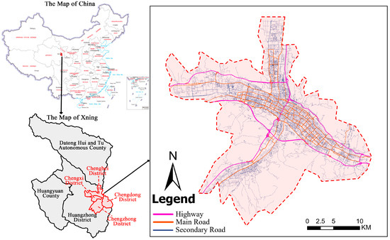
Figure 1. Overview of study area.

2.2. Research Framework

As illustrated in Figure 2, the research framework is systematically organized into six distinct steps: (1) CEs Estimation, where the dependent variable is constructed through spatial downscaling followed by seasonal and zero-error corrections to ensure precision. (2) Variable Construction, which generates the explanatory variable set by extracting visual features from SVIs via semantic segmentation and integrating them with POI indices. (3) Feature Screening, which rigorously ensures the independence of selected variables by utilizing Pearson correlation analysis and Variance Inflation Factor (VIF) tests to eliminate multicollinearity. (4) Geographically Weighted XGBoost Modeling, which establishes the core framework using adaptive bandwidths to capture local spatial heterogeneity. (5) Performance Evaluation, validating the model’s superiority and reliability by comparing the GW-XGBoost model against 12 machine learning baselines and conducting residual spatial autocorrelation tests. (6) Interpretability Analysis, utilizing the SHAP method to decode the “black box” mechanism by quantifying global feature contributions and visualizing local driving factors.

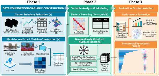
Figure 2. Schematic diagram of the research methodology.

2.3. Neighborhood Carbon Emissions Calculation

Nighttime light (NTL) intensity serves as a well-established proxy for human activity intensity, exhibiting a strong linear correlation with CEs [38]. Consequently, this study utilizes neighborhood CEs data for Qinghai Province (2013–2023) derived from the Multi-resolution Emission Inventory model for Climate and air pollution research (MEIC, http://meicmodel.org.cn, accessed on 21 June 2025) [39]. For NTL, we employed the NPP/VIIRS-like dataset developed by Chen et al. [40], which offers a temporally consistent and spatially continuous time series at a 500 m resolution.

To ensure estimation accuracy at the grid cell level, we adopted a linear regression model without an intercept, consistent with the methodology of Wu et al. [41]. This constraint ensures that pixels with a Digital Number value of zero are strictly assigned a calibrated value of zero, thereby eliminating background noise. Additionally, pixels covering water bodies were excluded from the analysis to mitigate potential light blooming effects. The fitting formula is defined as follows:

$${CS}_k=a\times T{DN}_k$$

(1)

where ${CS}_k$ represents the simulated neighborhood CEs for the year $k$, and ${TDN}_k$ denotes the total sum of $DN$ values for nighttime lights in the year $k$.

The regression yielded a fitting coefficient of $a=104.809$ with an R² of 0.913, confirming the model’s validity as consistent with Wu et al. [41], who established that R² values exceeding 0.9 indicate high accuracy in NTL-based inversions.

Based on the proportion of the total retail sales of consumer goods by urban residents in Xining City in June 2018 relative to the full year, this study takes 0.066 of the 2018 annual residential CEs to represent the residential CEs of Xining in June. The data source is the Xining National Economic Monthly Report.

To maintain the consistency of spatial statistical units and further improve simulation accuracy, the simulated CEs for pixel units were corrected using the provincial zero-error method [42]. The spatialized CEs data were calculated as follows:

$$C_{s,i,k}={\displaystyle \frac{{CE}_k}{{CS}_k}}\times {\displaystyle \frac{C_{x,i,k}}{S_i}}$$

(2)

where $C_{s,i,k}$ is the corrected neighborhood CEs density for grid $i$ in year $k$, ${CE}_k$ is the total neighborhood CEs for year $k$, ${CS}_k$ is the predicted total neighborhood CEs for year $k$, $S_i$ indicates the area of grid $i$, and $C_{x,i,k}$ is the predicted CEs value for grid $i$ in year $k$.

2.4. Data Acquisition and Variable Construction

2.4.1. SVI Acquisition and Sampling Strategy

Baidu Maps, one of the largest online map providers in China, provides multi-angle SVIs. This study downloaded Baidu SVIs through the Baidu Maps server. Specifically, road network data for Xining was obtained from OpenStreetMap (OSM), and sampling points were established at 50 m intervals. Using the Baidu server, 360° panoramic SVIs were collected at a fixed height (https://lbsyun.baidu.com/, accessed on 1 May 2025). All parameters were kept consistent, including heading, coordinates, resolution, and horizontal field of view.

To ensure data representativeness, we queried the historical availability of SVIs for all designated sampling points (Table 1). The year 2018 offered the most comprehensive spatial coverage with 8037 images, significantly surpassing previous years (e.g., 6514 images in 2014 and 3934 images in 2016). Crucially, SVI updates for the study area were negligible after 2018, with only sporadic records available for 2019 ($N=27$) and 2021 ($N=2$). Consequently, a total of 8037 images, each with a resolution of $1024\times 512$ pixels in JPG format, were selected for the final dataset. These samples were captured between June and July 2018, representing the most recent and complete visual record available for the city. In addition, we conducted field observations and on-site comparisons, indicating that the main street layouts and built environments in the central district of Xining have not undergone significant reconstruction or large-scale demolition since 2018. Therefore, the visual features captured in 2018 remain representative.

Table 1. Temporal distribution statistics of SVI data in the central district of Xining.

Year	May	June	July	August	Sum
2014	6514	None	None	None	6514
2015	None	1397	None	None	1397
2016	None	None	None	3934	3934
2018	None	7656	381	None	8037
2019	None	None	27	None	27
2021	None	None	2	None	2

2.4.2. Semantic Segmentation Based on Mask2Former

Mask2Former is a versatile image segmentation model based on a Transformer decoder that treats semantic segmentation as a set-prediction task, overcoming the limitations of traditional pixel-wise classification through a mask-classification mechanism [43]. In complex scenarios, Mask2Former demonstrates superior segmentation performance compared to traditional methods, significantly enhancing both accuracy and robustness. This provides a reliable technical foundation for urban environment analysis and autonomous driving scene understanding [44].

In this study, the Mask2Former model was employed to process the 8037 SVIs (Figure 3). The model was pre-trained on the Mapillary Vistas dataset to identify 66 distinct semantic categories within urban road spaces, such as Sky, Buildings, Roads, Fences, and Sidewalks [45]. To ensure optimal performance, this study adopted the model configuration equipped with a Swin-L (IN21k) backbone. Leveraging the global modeling capabilities of the Transformer, this configuration captures long-range contextual dependencies and achieves state-of-the-art results, recording a Mean Intersection over Union (mIoU) of 63.2% on the Mapillary Vistas Semantic Segmentation benchmark [46].

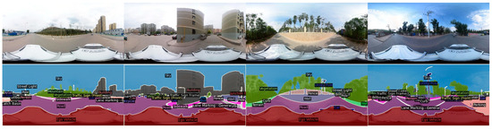
Figure 3. SVIs and their semantic segmentation results.

2.4.3. Data Cleaning and Visual Feature Selection

To ensure data quality, we performed a rigorous data cleaning process targeting the Ego Vehicle feature (the shooting vehicle itself). Since the size of the shooting vehicle within the SVIs should theoretically remain constant, significant deviations in its segmented area suggest potential segmentation errors or image anomalies. Therefore, we applied the Interquartile Range (IQR) method to identify and remove outliers based on the proportion of Ego Vehicle. This process reduced the valid sample size from 8037 to 6964.

Subsequently, given that not all visual features are suitable as independent variables, this study excluded features with a low frequency of occurrence (average proportion below 0.001%) and those not typical of urban road compositions. Following this screening, 19 visual features were selected.

2.4.4. Data Aggregation and POI Index Construction

To spatially align the heterogeneous data sources and bridge the resolution gap between micro-scale street views and macro-scale CEs, we adopted the grid method described by Zhang and Zeng [47], utilizing a grid size of $500\mathrm{m}\times 500\mathrm{m}$ as the basic analytical unit. Within this framework, the 19 selected visual features were aggregated into grid cells by calculating the average value of all sampling points within each unit. This strategy transforms discrete visual signals into a generalized representation of the neighborhood’s built environment character, making it statistically comparable to the grid-level CEs.

Furthermore, to capture the functional intensity and diversity of the built environment, this study utilized POI data for the year 2018, obtained from Amap. Based on the POI dataset, two key spatial indices were calculated for each grid cell:

The POI Density reflects the intensity of urban activities and is calculated as follow:

$$D_i={\displaystyle \frac{N_i}{A_i}}$$

(3)

where $N_i$ represents the total number of POIs in grid $i$, and $A_i$ is the area of the grid.

The POI Mixture measures functional diversity using the Shannon Entropy index, where a higher value indicates a more complex mixture of urban functions. It is calculated as follow:

$$M_i=-\sum _{k=1}^K{p}_{ik}\ln \left(p_{ik}\right)$$

(4)

where $K$ is the total number of POI categories, and $p_{ik}$ denotes the proportion of the $k$-th type of POI in grid $i$ relative to the total POIs.

Following the data aggregation and index construction, a descriptive statistical analysis was performed on the final dataset. Table 2 summarizes the statistical profiles for the dependent variable (CEs) and the 21 independent variables, comprising 19 visual features from SVIs and 2 POI indices.

Table 2. Summary of features.

Variables		Mean	Max	Min	StdDev.
Y	CEs	716.762	2451.520	33.655	467.784
X1	Curb	0.007	0.019	0.000	0.003
X2	Fence	0.010	0.074	0.000	0.009
X3	Guard Rail	0.002	0.028	0.000	0.005
X4	Barrier	0.003	0.061	0.000	0.006
X5	Wall	0.011	0.129	0.000	0.013
X6	Parking	0.002	0.027	0.000	0.003
X7	Pedestrian Area	0.001	0.028	0.000	0.003
X8	Road	0.141	0.195	0.053	0.022
X9	Sidewalk	0.010	0.052	0.000	0.008
X10	Building	0.070	0.399	0.000	0.053
X11	Lane Marking Crosswalk	0.002	0.107	0.000	0.005
X12	Lane Marking General	0.007	0.031	0.000	0.005
X13	Terrain	0.004	0.069	0.000	0.007
X14	Vegetation	0.122	0.356	0.003	0.058
X15	Billboard	0.005	0.042	0.000	0.006
X16	Pole	0.003	0.009	0.000	0.001
X17	Bus	0.002	0.053	0.000	0.005
X18	Car	0.027	0.127	0.000	0.019
X19	Truck	0.001	0.029	0.000	0.003
X20	POI Density	109.325	1104.000	0.000	164.186
X21	POI Mixture	6.424	10.026	0.000	2.786

2.5. GW-XGBoost Model

To strictly account for both spatial non-stationarity and nonlinear relationships in carbon emission modeling, this study adopts the GW-XGBoost framework proposed by Dong et al. [48]. Unlike traditional global models that assume a constant relationship across the study area, the GW-XGBoost model integrates the spatial weighting structure of Geographically Weighted Regression (GWR) into the ensemble learning architecture of XGBoost. This approach allows for the construction of localized models for each spatial unit, thereby capturing spatially varying driving mechanisms.

Prior to model construction, to eliminate the dimensional heterogeneity among different variables and ensure numerical stability, all continuous independent variables and the dependent variable were standardized using Z-score normalization. The formula is expressed as:

$$x_k^{\prime }={\displaystyle \frac{x_k-{\mu }_k}{{\sigma }_k}}$$

(5)

where $x_k^{\prime }$ represents the standardized value, $x_k$ is the original value of the $k$-th variable, ${\mu }_k$ is the mean, and ${\sigma }_k$ is the standard deviation.

Specifically, the implementation of this framework comprises two primary phases:

For each target grid $i$, a spatial weight $w_{ij}$ is assigned to neighboring observation $j$ based on the spatial distance. We calculated the Euclidean distance $d_{ij}$ and applied an adaptive Gaussian kernel to determine the weights:

$$w_{ij}={\displaystyle \frac{1}{\sqrt{2\pi }}}\exp \left(-{\displaystyle \frac{1}{2}}{\left({\displaystyle \frac{d_{ij}}{b_i}}\right)}^2\right)$$

(6)

where $b_i$ is the optimal bandwidth determined by the $k$-nearest neighbor method.

Based on the calculated spatial weights, a separate XGBoost regressor is trained for each grid $i$. The core distinction from the global XGBoost lies in the modification of the loss function to incorporate spatial heterogeneity. Adopting the least squares method (squared error loss), the objective for the local model at target grid $i$ is formulated to minimize the spatially weighted loss:

$$L_i={\displaystyle \frac{1}{2}}\sum _{j=1}^N{w}_{ij}{\left(y_j-{\widehat{y}}_j\right)}^2$$

(7)

where $N$ is the number of observations, and $w_{ij}$ represents the spatial weight of observation $j$ relative to target grid $i$. XGBoost optimizes this objective using a second-order Taylor expansion. Consequently, the spatial weights directly scale the first-order gradient ($g_j$) and second-order Hessian ($h_j$) for each observation $j$:

$$g_j={\displaystyle \frac{\partial L_i}{\partial {\widehat{y}}_j}}=w_{ij}\left({\widehat{y}}_j-y_j\right)$$

(8)

$$h_j={\displaystyle \frac{{\partial }^2{L}_i}{\partial {\widehat{y}}_j^2}}=w_{ij}$$

(9)

By weighting the gradients and Hessians, samples with higher spatial weights exert a stronger influence on the tree structure learning, thereby allowing the model to effectively capture local characteristics.

3. Results

3.1. Correlation Analysis of Features

To strictly evaluate the independence and validity of the selected indicators, this study calculated the Pearson correlation coefficients for the 21 explanatory variables. In the visualization, dark colors indicate stronger correlations, while lighter colors denote weak or no correlation (Figure 4). The Pearson correlation coefficient serves as a statistical metric to quantify the degree and direction of linear relationships between variables.

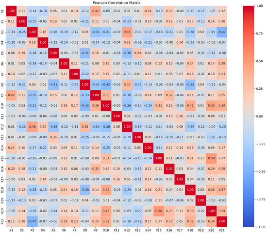
Figure 4. Pearson correlation matrix of features.

As shown in the correlation matrix, the overall correlation among the variables is relatively weak, with the absolute values of the majority of coefficients falling below 0.5. Specifically, Billboard and POI Density exhibited the strongest positive correlation with a coefficient of 0.50. This relationship highlights a logical coupling between visual form and urban function, as commercial areas with high POI Density of interest typically feature a higher concentration of outdoor advertising. Conversely, Building and Road showed a significant negative correlation of −0.42. This suggests that in dense urban canyons where buildings occupy a dominant portion of the visual field, the proportion of visible road surface tends to decrease due to perspective occlusion.

To further rigorously rule out potential multicollinearity issues that could distort the regression model, the Variance Inflation Factor (VIF) was calculated for all predictors. Academic standards generally consider a VIF value below 10 to indicate no severe multicollinearity. The results show that the VIF values for all 21 features are well below the strict threshold of 5 (Table 3). The highest VIFs were observed for Building and Road, while the VIFs of the remaining features were almost all below 2.0. These results confirm that the selected multidimensional features possess a high degree of independence.

Table 3. Multicollinearity analysis of explanatory variables.

Feature	VIF	Feature	VIF
Building	3.691	Billboard	1.537
Road	3.535	Curb	1.517
Guard Rail	2.181	Fence	1.385
Vegetation	1.924	Barrier	1.353
POI Density	1.901	Pole	1.305
POI Mixture	1.859	Lane Marking Crosswalk	1.234
Lane Marking General	1.853	Parking	1.185
Sidewalk	1.823	Pedestrian Area	1.153
Wall	1.819	Bus	1.144
Car	1.679	Truck	1.125
Terrain	1.605

3.2. Comparative Analysis of Model Performance

To comprehensively evaluate the prediction accuracy and generalization capability, this study selected 12 mainstream machine learning algorithms as benchmarks for comparative analysis. In terms of experimental design, the dataset was randomly partitioned into a training set (80%) for model construction and a testing set (20%) for performance evaluation. Metrics including R², RMSE, and MAE were calculated on the testing set to ensure a fair and rigorous assessment of the generalization performance across all baseline models.

Regarding the proposed GW-XGBoost model, a more refined parameter tuning strategy was adopted to precisely capture spatial non-stationarity. By combining grid search with 5-fold cross-validation, the optimal hyperparameter combination for the underlying XGBoost model (version 3.0.2) was identified as follows: n_estimators = 300, learning_rate = 0.05, max_depth = 3, and both subsample and colsample_bytree = 0.8. Furthermore, regarding the bandwidth—the critical spatial parameter determining the scope of local models—this study adaptively determined the optimal bandwidth to be the 50 nearest neighbors by minimizing the Leave-One-Out Cross-Validation error. This configuration achieves an optimal balance between local fitting accuracy and model stability.

Table 4 details the performance evaluation results of all models. The comparison reveals that traditional global models struggle to fully explain the spatial variability of CEs. Linear models demonstrated relatively limited fitting capability ($R^2\approx 0.644$), and while global ensemble models represented by Global XGBoost showed improvement ($R^2=0.729$, $RMSE=302.137$), there remains room for enhancement. In contrast, the GW-XGBoost model demonstrated significant superiority by incorporating spatial weighting. It achieved a median local R² of 0.819 and a median RMSE of 102.532, representing a substantial 66% reduction in prediction error compared to the best-performing global model (Global XGBoost). Most importantly, even the minimum fitting goodness (Min $R^2=0.733$) observed among the local GW-XGBoost models surpassed the maximum performance of all global baselines. This result strongly validates the necessity of accounting for spatial heterogeneity in carbon emission modeling.

Table 4. Comparison of model performance.

Index	Model		R2	RMSE	MAE
1	Linear		0.644	346.271	294.758
2	Lasso		0.644	346.286	294.762
3	Ridge		0.643	346.538	294.990
4	Decision Tree		0.464	424.620	319.133
5	Random Forest		0.700	317.996	276.593
6	AdaBoost		0.646	345.128	307.197
7	Backpropagation		0.601	366.283	277.673
8	Artificial Network		0.655	340.775	275.531
9	XGBoost		0.725	304.233	256.322
10	SVM		0.488	415.281	318.050
11	GBDT		0.695	320.293	269.581
12	Catboost		0.715	309.510	255.837
13	GW-XGBoost *	Max	0.938	52.816	29.275
		Median	0.819	102.532	67.770
		Min	0.733	167.635	83.342

Note: * The best model selected.

Finally, to verify whether the model effectively addressed spatial dependence, a spatial autocorrelation test was conducted on the residuals of the GW-XGBoost model (calculated as the difference between observed and predicted values). The results indicate a global Moran’s I index of only 0.0337 (p-value = 0.0010). Although the significant p-value suggests that the residuals are not strictly random in a statistical sense, this is primarily attributed to the high sensitivity of the test given the large sample size. In terms of effect size, the extremely low Moran’s I value indicates that the vast majority of spatial autocorrelation has been successfully eliminated by the model. Consequently, the residuals exhibit a quasi-random distribution characteristic, further confirming the validity of the model.

3.3. Feature Contribution Analysis

To quantify the overall contribution of built environment features to CEs, we aggregated the absolute SHAP values from all local models. Figure 5 illustrates the global feature importance ranking based on the mean absolute SHAP values. The results reveal a clear hierarchy in the feature importance, characterized by the dominance of socioeconomic functional attributes over physical visual features. POI Density and POI Mixture emerge as the two most substantial influencers, respectively. Notably, the contribution of POI Density is nearly double that of the highest-ranking visual feature. Among the visual indicators, Lane Marking General, Building, and Wall exert the most significant impact.

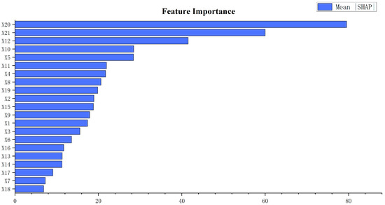
Figure 5. Feature importance.

The SHAP summary plot elucidates the directionality of feature influence, specifically examining whether a feature promotes or inhibits neighborhood CEs (Figure 6). A distinct positive association is observed for the top-ranking variables. High feature values for POI Density, POI Mixture, and Lane Marking General are predominantly concentrated on the positive side of the SHAP axis. This indicates that an increase in these indicators consistently contributes to elevated carbon emission predictions. Notably, Building exhibits an asymmetrical impact: while low feature values correspond to strongly negative SHAP values, high feature values cluster on the positive axis but remain relatively close to zero. This suggests that while the absence of buildings acts as a strong suppressor of emissions, high building density exerts a much less prominent positive drive compared to POI indicators.

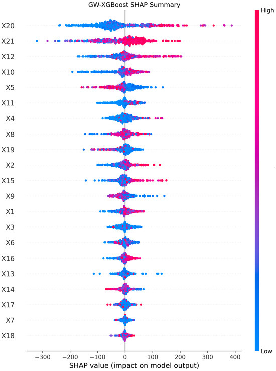
Figure 6. SHAP value summary plot.

In contrast, specific visual features exhibit an inhibitory effect on CEs. Wall and Sidewalk display a reverse pattern, where high feature values correspond to negative SHAP values on the left side of the axis. This implies that streetscapes dominated by these elements, which potentially indicate enclosed boundaries or pedestrian-oriented environments, tend to reduce the model’s predicted emissions.

3.4. Spatial Heterogeneity of Feature Impacts

To reveal the local spatial variations in how built environment features influence CEs, we visualized the SHAP values of the top four contributors (Figure 7). In these maps, red indicates a positive SHAP value, blue indicates a negative SHAP value, and the color intensity reflects the magnitude of the impact.

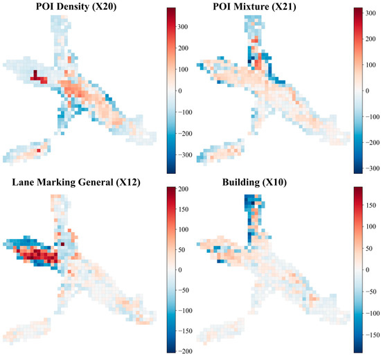
Figure 7. Spatial distribution of SHAP values for key features.

The spatial distribution of POI Density exhibits a distinct core–periphery pattern, characterized by positive values in the city center and negative values on the outskirts. Notably, distinct patches of deep red emerge in the western sector against a predominantly pale background. These isolated high-value clusters align with to Xining’s major commercial districts, indicating that dense concentrations of facilities act as powerful, localized drivers of emissions even within generally low-impact zones. Similarly, POI Mixture shares this core–periphery structure but exhibits subtle regional variations in intensity. The northern and western regions display relatively higher saturation compared to the lighter southern and eastern areas. This visual distinction suggests that the influence of functional diversity on CEs is slightly more pronounced in these sectors, although the overall spatial differentiation remains moderate.

Regarding streetscape visual features, Lane Marking General reveals a striking spatial anomaly in the western region, which exhibits significantly deeper colors than other areas. This pattern indicates that the model assigns substantially higher weights to this feature specifically in the western sector. For the Building feature, the most distinct visual patterns are concentrated in the northern region. Specifically, the urban fringe in the north is marked by deep blue clusters. These areas correspond to the city’s boundary where buildings are sparse or non-existent. The model accurately captures this characteristic, assigning strongly negative SHAP values to indicate that the lack of built volume significantly attenuates predicted CEs in these marginal zones.

4. Discussion

4.1. Spatial Residual Analysis of GW-XGBoost Model

To rigorously evaluate the local predictive performance of the GW-XGBoost model, we calculated the prediction residuals (defined as $Residual= Observed-Predicted$) for each 500 m grid and mapped their spatial distribution alongside a frequency histogram (Figure 8).

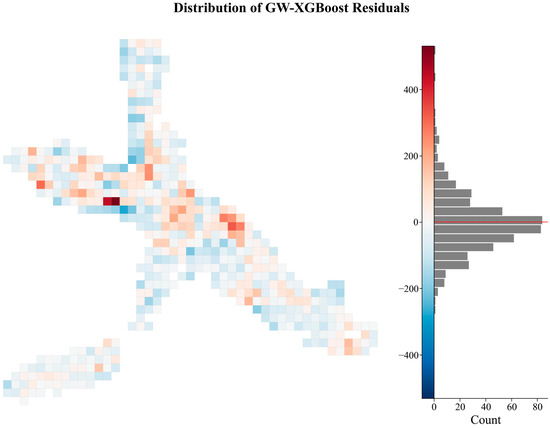
Figure 8. Spatial distribution and frequency histogram of prediction residuals.

The histogram demonstrates that the residuals follow a distribution that approximates a normal distribution, with a sharp peak centered around zero. This indicates that for the vast majority of grids, the predicted values are highly consistent with the observed CEs.

Despite this robust overall fit, the spatial map reveals distinct patterns of heterogeneity. A higher frequency of negative residuals is observed in the urban fringe compared to the center, although their absolute values remain generally small. This suggests a slight tendency of the model to overestimate emissions in transitional zones. This phenomenon aligns with the findings of Shi et al. [19], reflecting the complexity of carbon emission factors in urban peripheral regions which the model may not have fully captured. Conversely, positive residuals are predominantly concentrated in the urban interior, particularly in high-density residential clusters, implying that the model may slightly underestimate carbon intensity in complex environments where anthropogenic activities are most intense. Notably, the analysis highlights two distinct outlier points with significantly high positive residuals in the western sector, corresponding to the city’s major commercial districts. Here, the dense concentration of commercial complexes creates extreme emission values. Although the model predicted high levels, it underestimated the peak magnitude, resulting in a smoothing effect on extreme values. In summary, while minor deviations exist, the residual analysis confirms that the GW-XGBoost model effectively captures the overall spatial structure of and variation in CEs across the study area.

4.2. Association Between Features and Neighborhood Carbon Emissions

The analysis of SHAP values reveals the intrinsic associations between built environment features and neighborhood CEs. We identified POI Density and POI Mixture as the most critical positive drivers of CEs. This result indicates that in predicting CEs, functional attributes reflecting urban socioeconomic vitality play a more dominant role than purely visual features of the built environment. Lane Marking General, ranking as the third largest contributor, exhibits a significant positive impact. High densities of lane markings are typically found on high-grade roads within urban cores or transportation hubs. Rather than merely signifying well-developed infrastructure, this feature serves as a direct proxy for high traffic pressure and motorization levels, thereby showing a positive correlation with carbon emission intensity.

Building generally exhibits a positive correlation. However, it is worth noting that the magnitude of its impact displays a distinct asymmetry: the negative impact derived from low building density is significantly more pronounced than the positive impact of high building density. Wall shows a negative correlation, a finding that contradicts the results of Zhang et al. [49]. Wall also shows a negative correlation. It is important to clarify that the walls identified in this study refer primarily to solid surfaces without windows. Such visual features often appear in older or less vibrant urban areas with lower population activity, leading to lower neighborhood CEs. Furthermore, Sidewalk demonstrates a clear negative correlation. As noted by Dong et al. [50], well-developed sidewalk infrastructure effectively promotes low-carbon travel modes such as walking and jogging. By substituting for short-distance vehicular trips, sidewalks play a positive role in mitigating neighborhood CEs.

4.3. Neighborhood Environment Optimization Strategies from a Low-Carbon Perspective

This study reveals a significant association between built environment features and CEs, providing data-driven theoretical support for low-carbon street design. Street design oriented toward low-carbon development should be approached from three dimensions: spatial morphology optimization, traffic organization synergy, and ecological greening. By precisely responding to the mechanism linking visual features to CEs, planners can construct low-energy and high-resilience street spaces.

In the design of street spaces, priority should be given to optimizing the functional mix and rationally managing building density. Since POI Mixture is identified as a critical driver, planning strategies should advocate for mixed land-use patterns. This aligns with the findings of Zhang et al. [51], who confirmed that building type and Floor Area Ratio (FAR) are key indicators influencing carbon emission intensity, suggesting that optimizing these metrics serves as an effective spatial management pathway for achieving urban carbon reduction goals. Consequently, planning efforts should promote both functional mixing and moderately intensive development. By integrating diverse functions such as commercial, residential, and recreational uses, residents’ dependence on long-distance vehicular travel can be significantly reduced.

Regarding traffic organization, a balance must be sought between satisfying traffic demand and reducing CEs. Optimizing the layout and routing of bus stops can enhance the accessibility and attractiveness of public transportation [52]. Technological means, such as traffic light regulation and dynamic lane allocation, can alleviate congestion, improve road efficiency, and reduce vehicle idling emissions. Furthermore, street signage and landscape guidance can encourage residents to choose public or non-motorized transportation, reducing traffic emissions from the demand side [53].

Since Sidewalk demonstrates a clear negative correlation with CEs, improving the quality and comfort of the walking environment is a pivotal strategy. Street greening should be strategically integrated with pedestrian infrastructure to create a comfortable, shaded, and aesthetically pleasing travel environment. This approach effectively encourages residents to substitute short-distance vehicular trips with walking or jogging, thereby reducing emissions through both ecological functions and behavioral patterns [54].

5. Conclusions and Limitations

5.1. Conclusions

This study established a high-precision framework for estimating and interpreting neighborhood-scale CEs in the central urban area of Xining by integrating multi-source geospatial big data, specifically SVIs and POI data, with the GW-XGBoost model. By decoding the complex non-linear and spatially heterogeneous relationships between the built environment and CEs, this research provides novel insights for low-carbon urban planning in ecologically fragile plateau regions.

First, the GW-XGBoost model demonstrated significant advantages over traditional global machine learning models. By incorporating spatial weighting to account for local spatial non-stationarity, the model achieved a median R² of 0.819. The residual analysis further confirmed the model’s reliability, with errors exhibiting a quasi-random distribution, proving its efficacy in capturing the spatial variation in CEs at a fine granular level. Second, the interpretability analysis based on SHAP values revealed that socioeconomic functional attributes exert a more decisive influence on CEs than purely visual physical features. POI Density and POI Mixture were identified as the top two positive drivers, highlighting that the intensity and diversity of urban activities are the primary sources of carbon emission heterogeneity. Third, among streetscape visual features, Lane Marking General served as a strong proxy for traffic pressure, exhibiting a significant positive correlation with emissions, particularly in the western commercial districts. Conversely, Sidewalks demonstrated a clear negative correlation, supporting the premise that high-quality pedestrian infrastructure mitigates emissions by promoting active travel modes.

In conclusion, this study bridges the gap between micro-scale environmental perception and macro-scale carbon assessment. While the observed effect sizes are context-dependent, the methodological framework established herein is transferable to other cities. The findings suggest that future low-carbon urban renewal strategies in Xining should prioritize the optimization of land-use functionality and the enhancement of active travel systems. Specifically, planning efforts should focus on fostering multifunctional mixed-use districts and upgrading pedestrian environments to reduce automobile dependence. These data-driven insights offer a scientific basis for constructing resilient and low-carbon urban spaces on the Tibetan Plateau.

5.2. Limitations

Despite its contributions, this study remains subject to certain limitations, primarily in the following three areas.

First, temporal and spatial constraints exist. A mismatch remains between the summer-acquired SVIs and annual CEs, potentially overlooking seasonal variations. Additionally, while the 500 m grid improves resolution, it may still obscure fine-grained neighborhood details, and static imagery cannot capture dynamic real-time emission interactions.

Second, SVI coverage is limited by road accessibility. Vehicle-based sampling inevitably excludes interior courtyards and narrow alleys. Although we integrated POI data to compensate for functional blind spots, the visual character of these non-road environments remains partially unobserved.

Finally, generalizability and causal inference are constrained. Xining’s unique valley topography influences visual patterns differently than flat cities, limiting transferability. Furthermore, the cross-sectional design captures associations rather than causality; future research requires longitudinal analysis and multi-city comparisons to validate these mechanisms.

References

- Liu, Z.; Deng, Z.; Davis, S.; Ciais, P. Monitoring Global Carbon Emissions in 2022. Nat. Rev. Earth Environ. 2023, 4, 205–206. [Google Scholar] [CrossRef]
- Cheng, H.; Wu, B.; Jiang, X. Study on the Spatial Network Structure of Energy Carbon Emission Efficiency and Its Driving Factors in Chinese Cities. Appl. Energy 2024, 371, 123689. [Google Scholar] [CrossRef]
- Wang, J.; Azam, W. Natural Resource Scarcity, Fossil Fuel Energy Consumption, and Total Greenhouse Gas Emissions in Top Emitting Countries. Geosci. Front. 2024, 15, 101757. [Google Scholar] [CrossRef]
- Zhao, Q.; Jiang, M.; Zhao, Z.; Liu, F.; Zhou, L. The Impact of Green Innovation on Carbon Reduction Efficiency in China: Evidence from Machine Learning Validation. Energy Econ. 2024, 133, 107525. [Google Scholar] [CrossRef]
- Wang, X.; Zhao, G.; He, C.; Wang, X.; Peng, W. Low-Carbon Neighborhood Planning Technology and Indicator System. Renew. Sustain. Energy Rev. 2016, 57, 1066–1076. [Google Scholar] [CrossRef]
- Wang, Y.; Fang, X.; Yin, S.; Chen, W. Low-Carbon Development Quality of Cities in China: Evaluation and Obstacle Analysis. Sustain. Cities Soc. 2021, 64, 102553. [Google Scholar] [CrossRef]
- Gan, J.; Li, L.; Xiang, Q.; Ran, B. A Prediction Method of GHG Emissions for Urban Road Transportation Planning and Its Applications. Sustainability 2020, 12, 10251. [Google Scholar] [CrossRef]
- Wu, R.; Zhang, Y.; Cai, Y.; Wang, S. Impacts of Multi-Scale Built Environment on Transportation Carbon Emissions: A Guangzhou Case. Cities 2026, 169, 106573. [Google Scholar] [CrossRef]
- Zhou, K.; Zheng, X.; Huang, S.; Li, H.; Yin, H. Quantifying the Combined and Individual Impacts of Climate and Human Activity on the Urban Green Space Carbon Sink Capacity in Beijing. Sustain. Cities Soc. 2025, 122, 106253. [Google Scholar] [CrossRef]
- Yang, Z.; Fan, Y.; Zheng, S. Determinants of Household Carbon Emissions: Pathway toward Eco-Community in Beijing. Habitat Int. 2016, 57, 175–186. [Google Scholar] [CrossRef]
- Zhang, Y.; Li, Y.; Zhang, F. Multi-Level Urban Street Representation with Street-View Imagery and Hybrid Semantic Graph. ISPRS J. Photogramm. Remote. Sens. 2024, 218, 19–32. [Google Scholar] [CrossRef]
- Lu, Y. Using Google Street View to Investigate the Association between Street Greenery and Physical Activity. Landsc. Urban Plan. 2019, 191, 103435. [Google Scholar] [CrossRef]
- Guan, H.; Zhang, W.; Huang, B.; Xu, Y.; Hong, W. How Urban Street-Scape Visual Features Influence Carbon Emissions from Residents Visiting Urban Parks: A Case Study of Shenzhen, China. Landsc. Urban Plan. 2026, 266, 105531. [Google Scholar] [CrossRef]
- Aikoh, T.; Homma, R.; Abe, Y. Comparing Conventional Manual Measurement of the Green View Index with Modern Automatic Methods Using Google Street View and Semantic Segmentation. Urban For. Urban Green. 2023, 80, 127845. [Google Scholar] [CrossRef]
- Tang, F.; Zeng, P.; Wang, L.; Zhang, L.; Xu, W. Urban Perception Evaluation and Street Refinement Governance Supported by Street View Visual Elements Analysis. Remote Sens. 2024, 16, 3661. [Google Scholar] [CrossRef]
- Li, X.; Ratti, C.; Seiferling, I. Quantifying the Shade Provision of Street Trees in Urban Landscape: A Case Study in Boston, USA, Using Google Street View. Landsc. Urban Plan. 2018, 169, 81–91. [Google Scholar] [CrossRef]
- Zhang, L.; Wang, L.; Wu, J.; Li, P.; Dong, J.; Wang, T. Decoding Urban Green Spaces: Deep Learning and Google Street View Measure Greening Structures. Urban For. Urban Green. 2023, 87, 128028. [Google Scholar] [CrossRef]
- Chen, Z.; Zou, T.; Xu, Z.; Zhang, Y.; Chen, N. SAGE-GSAN: A Graph-Based Method for Estimating Urban Taxi CO Emissions Using Street View Images. J. Clean. Prod. 2024, 474, 143543. [Google Scholar] [CrossRef]
- Shi, W.; Xiang, Y.; Ying, Y.; Jiao, Y.; Zhao, R.; Qiu, W. Predicting Neighborhood-Level Residential Carbon Emissions from Street View Images Using Computer Vision and Machine Learning. Remote Sens. 2024, 16, 1312. [Google Scholar] [CrossRef]
- Wu, L.; Liu, X.; Zhang, X.; Wang, R.; Guo, Z. End-to-End Deep Learning for Pollutant Prediction Using Street View Images. Urban Clim. 2025, 60, 102368. [Google Scholar] [CrossRef]
- Liu, X.; Song, M.; Wang, S.; Xu, X.; Li, H. On Innovation Infrastructure and Industrial Carbon Emissions: Nonlinear Correlation and Effect Mechanism. Appl. Energy 2024, 375, 124079. [Google Scholar] [CrossRef]
- Cai, B.; Zhang, L. Urban CO2 Emissions in China: Spatial Boundary and Performance Comparison. Energy Policy 2014, 66, 557–567. [Google Scholar] [CrossRef]
- Zhang, X.; Wang, Q.; Jia, X.; Zhao, Y.; Zhou, H.; Lin, B.; Zhang, C. Feature Evaluation, Regression Prediction and Scenario Analysis of Carbon Emissions from City Building Operations: Evidence from 362 Chinese Cities. Sustain. Cities Soc. 2025, 134, 106911. [Google Scholar] [CrossRef]
- Liu, W.; Yue, X.; Wang, X.; Lin, Z.; Yao, X.; Xu, Z. Spatial Distribution and Driving Factors of Carbon Emission in a Furnace City Using Luojia1–01 Nighttime Data and Optimal Parameters-Based Geodetector. Urban Clim. 2025, 61, 102462. [Google Scholar] [CrossRef]
- Zhao, L.; Zhang, C.; Wang, Q.; Yang, C.; Zhou, W. Spatio-Temporal Variations of Land Use Carbon Emissions and Its Low Carbon Strategies for Coastal Areas in China with Nighttime Lighting Data. J. Environ. Manag. 2025, 385, 125651. [Google Scholar] [CrossRef]
- Zhang, X.; Cai, Z.; Song, W.; Yang, D. Mapping the Spatial-Temporal Changes in Energy Consumption-Related Carbon Emissions in the Beijing-Tianjin-Hebei Region via Nighttime Light Data. Sustain. Cities Soc. 2023, 94, 104476. [Google Scholar] [CrossRef]
- Cai, B.; Li, W.; Dhakal, S.; Wang, J. Source Data Supported High Resolution Carbon Emissions Inventory for Urban Areas of the Beijing-Tianjin-Hebei Region: Spatial Patterns, Decomposition and Policy Implications. J. Environ. Manag. 2018, 206, 786–799. [Google Scholar] [CrossRef]
- Wang, H.; Zeng, W. Revealing Urban Carbon Dioxide (CO2) Emission Characteristics and Influencing Mechanisms from the Perspective of Commuting. Sustainability 2019, 11, 385. [Google Scholar] [CrossRef]
- Cai, M.; Shi, Y.; Ren, C.; Yoshida, T.; Yamagata, Y.; Ding, C.; Zhou, N. The Need for Urban Form Data in Spatial Modeling of Urban Carbon Emissions in China: A Critical Review. J. Clean. Prod. 2021, 319, 128792. [Google Scholar] [CrossRef]
- Hong, X.; Zhang, C.; Tian, Y.; Zhu, Y.; Hao, Y.; Liu, C. First TanSat CO2 Retrieval over Land and Ocean Using Both Nadir and Glint Spectroscopy. Remote Sens. Environ. 2024, 304, 114053. [Google Scholar] [CrossRef]
- Sheng, M.; Hou, Y.; Song, H.; Ye, X.; Lei, L.; Ma, P.; Zeng, Z.-C. Estimating Anthropogenic CO2 Emissions from China’s Yangtze River Delta Using OCO-2 Observations and WRF-Chem Simulations. Remote Sens. Environ. 2025, 316, 114515. [Google Scholar] [CrossRef]
- Kuze, A.; Nakamura, Y.; Oda, T.; Yoshida, J.; Kikuchi, N.; Kataoka, F.; Suto, H.; Shiomi, K. Examining Partial-Column Density Retrieval of Lower-Tropospheric CO2 from GOSAT Target Observations over Global Megacities. Remote Sens. Environ. 2022, 273, 112966. [Google Scholar] [CrossRef]
- Yang, S.; Lei, L.; Zeng, Z.; He, Z.; Zhong, H. An Assessment of Anthropogenic CO2 Emissions by Satellite-Based Observations in China. Sensors 2019, 19, 1118. [Google Scholar] [CrossRef] [PubMed]
- Hakkarainen, J.; Ialongo, I.; Tamminen, J. Direct Space-based Observations of Anthropogenic CO2 Emission Areas from OCO-2. Geophys. Res. Lett. 2016, 43, 11400–11406. [Google Scholar] [CrossRef]
- Zhou, X.; Wanghe, K.; Jiang, H.; Ahmad, S.; Zhang, D. Construction of Green Infrastructure Networks Based on the Temporal and Spatial Variation Characteristics of Multiple Ecosystem Services in a City on the Tibetan Plateau: A Case Study in Xining, China. Ecol. Indic. 2024, 163, 112139. [Google Scholar] [CrossRef]
- Wei, J.; Tian, M.; Wang, X. Spatiotemporal Variation in Land Use and Ecosystem Services during the Urbanization of Xining City. Land 2023, 12, 1118. [Google Scholar] [CrossRef]
- Wang, Y.; Song, C.; Cheng, C.; Wang, H.; Wang, X.; Gao, P. Modelling and Evaluating the Economy-Resource-Ecological Environment System of a Third-Polar City Using System Dynamics and Ranked Weights-Based Coupling Coordination Degree Model. Cities 2023, 133, 104151. [Google Scholar] [CrossRef]
- Jin, T.; Zhang, P.; Zhu, A.; Liu, S.; Zhou, N.; Guo, H. Decoding the Seasonal Variations in the Synergistic Effects of Multidimensional Urban Morphology on Carbon Emissions and Air Temperature. Build. Environ. 2025, 286, 113750. [Google Scholar] [CrossRef]
- Geng, G.; Liu, Y.; Liu, Y.; Liu, S.; Cheng, J.; Yan, L.; Wu, N.; Hu, H.; Tong, D.; Zheng, B.; et al. Efficacy of China’s Clean Air Actions to Tackle PM2.5 Pollution between 2013 and 2020. Nat. Geosci. 2024, 17, 987–994. [Google Scholar] [CrossRef]
- Chen, Z.; Yu, B.; Yang, C.; Zhou, Y.; Yao, S.; Qian, X.; Wang, C.; Wu, B.; Wu, J. An Extended Time Series (2000–2018) of Global NPP-VIIRS-like Nighttime Light Data from a Cross-Sensor Calibration. Earth Syst. Sci. Data 2021, 13, 889–906. [Google Scholar] [CrossRef]
- Wu, H.; Yang, Y.; Li, W. Dynamic Spatiotemporal Evolution and Spatial Effect of Carbon Emissions in Urban Agglomerations Based on Nighttime Light Data. Sustain. Cities Soc. 2024, 113, 105712. [Google Scholar] [CrossRef]
- Zhou, Y.; Chen, M.; Tang, Z.; Zhao, Y. City-Level Carbon Emissions Accounting and Differentiation Integrated Nighttime Light and City Attributes. Resour. Conserv. Recycl. 2022, 182, 106337. [Google Scholar] [CrossRef]
- Zhou, M.; Yin, P.; Cui, J.; Lou, H.; Yang, Z.; Liu, J.; Peng, C. From Pixels to 3D Models: Mask2Former-Driven Automated Reconstruction of Jiangnan Traditional Villages Using Remote Sensing Images. J. Build. Eng. 2025, 114, 114277. [Google Scholar] [CrossRef]
- Sánchez, I.A.V.; Labib, S.M. Accessing Eye-Level Greenness Visibility from Open-Source Street View Images: A Methodological Development and Implementation in Multi-City and Multi-Country Contexts. Sustain. Cities Soc. 2024, 103, 105262. [Google Scholar] [CrossRef]
- Neuhold, G.; Ollmann, T.; Bulò, S.R.; Kontschieder, P. The Mapillary Vistas Dataset for Semantic Understanding of Street Scenes. In Proceedings of the 2017 IEEE International Conference on Computer Vision (ICCV), Venice, Italy, 22–29 October 2017; pp. 5000–5009. [Google Scholar]
- Cheng, B.; Misra, I.; Schwing, A.G.; Kirillov, A.; Girdhar, R. Masked-Attention Mask Transformer for Universal Image Segmentation. In Proceedings of the 2022 IEEE/CVF Conference on Computer Vision and Pattern Recognition (CVPR), New Orleans, LA, USA, 18–24 June 2022; pp. 1280–1289. [Google Scholar]
- Zhang, W.; Zeng, H. Spatial Differentiation Characteristics and Influencing Factors of the Green View Index in Urban Areas Based on Street View Images: A Case Study of Futian District, Shenzhen, China. Urban For. Urban Green. 2024, 93, 128219. [Google Scholar] [CrossRef]
- Dong, S.; Wang, Y.; Wang, C.; Dou, M.; Gong, J. Discovering the Nonlinear Association between the Built Environment and Metro Ridership: Global and Local Perspectives. Cities 2026, 169, 106561. [Google Scholar] [CrossRef]
- Zhang, Y.; Sun, T.; Wang, L.; Huang, B.; Pan, X.; Song, W.; Wang, K.; Xiong, X.; Xu, S.; Yao, L.; et al. Portraying On-Road CO2 Concentrations Using Street View Panoramas and Ensemble Learning. Sci. Total Environ. 2024, 946, 174326. [Google Scholar] [CrossRef]
- Dong, L.; Jiang, H.; Li, W.; Qiu, B.; Wang, H.; Qiu, W. Assessing Impacts of Objective Features and Subjective Perceptions of Street Environment on Running Amount: A Case Study of Boston. Landsc. Urban Plan. 2023, 235, 104756. [Google Scholar] [CrossRef]
- Zhang, N.; Luo, Z.; Liu, Y.; Feng, W.; Zhou, N.; Yang, L. Towards Low-Carbon Cities through Building-Stock-Level Carbon Emission Analysis: A Calculating and Mapping Method. Sustain. Cities Soc. 2022, 78, 103633. [Google Scholar] [CrossRef]
- Li, X.; Lv, T.; Qu, D. Assessing Carbon Emissions from Urban Road Transport through Composite Framework. Sustain. Energy Technol. Assess. 2025, 73, 104151. [Google Scholar] [CrossRef]
- Muñiz, I.; Sánchez, V. Urban Spatial Form and Structure and Greenhouse-Gas Emissions from Commuting in the Metropolitan Zone of Mexico Valley. Ecol. Econ. 2018, 147, 353–364. [Google Scholar] [CrossRef]
- Ma, X.; Chau, C.K.; Lai, J.H.K. Critical Factors Influencing the Comfort Evaluation for Recreational Walking in Urban Street Environments. Cities 2021, 116, 103286. [Google Scholar] [CrossRef]
Disclaimer/Publisher’s Note: The statements, opinions and data contained in all publications are solely those of the individual author(s) and contributor(s) and not of MDPI and/or the editor(s). MDPI and/or the editor(s) disclaim responsibility for any injury to people or property resulting from any ideas, methods, instructions or products referred to in the content. |
© 2026 by the authors. Licensee MDPI, Basel, Switzerland. This article is an open access article distributed under the terms and conditions of the Creative Commons Attribution (CC BY) license.