A Simplified Method for Assessing Thermal Stresses During the Construction of Massive Monolithic Foundation Slabs Based on Temperatures at Three Points

Abstract

For massive monolithic foundation slabs, the risk of early cracking during construction is a pressing issue. This problem is primarily caused by thermal stresses arising from uneven heating of the structure during concrete curing and cooling. The most common approach to assessing thermal stresses is to express them through the temperature difference between the center and surface of the structure. However, this approach fails to take into account that heat transfer conditions on the upper and lower surfaces of the slab may differ. The purpose of this article is to derive calculation relationships that allow thermal stresses to be expressed through temperatures at three characteristic points on the slab: at the lower surface, in the middle of the slab, and at the upper surface. The resulting formulas were validated by comparison with the results of finite element analysis and an experiment presented in the work of other authors. Compared to the results of finite element analysis, the error in determining the maximum tensile stresses at the center of the slab is 0.4%. To assess the applicability limits of the resulting formulas, a series of finite element calculations were also performed for various slab thicknesses. It was established that for a slab thickness of up to 2 m, the error in determining stresses at three characteristic points using the authors’ formulas does not exceed 10%.

1. Introduction

The formation of temperature cracks during construction is a common problem in massive monolithic concrete structures under actual operating conditions [1]. Concrete structures that are completely free of cracks are, in fact, extremely rare. In the early stages of concrete elements or structures, heat is released during the hardening of the cement, causing the temperature of the concrete to rise. As the surface of the concrete cools, a temperature difference occurs: the outside of the concrete is colder than the center. Because of this, different parts of the concrete element expand unevenly. Temperature cracks appear if tensile stresses arise on the surface that exceed the permissible tensile strain for concrete due to the expansion of the center [2,3]. Additional tensile stresses can arise due to early compression caused by autogenous shrinkage [4,5]. Early cracking can also be caused by the following factors: the composition of the concrete mix, operating conditions, hydration rate, and hardening parameters of the material [2].

The consequences of temperature cracking include reduced strength and durability of the structure and the potential penetration of moisture and aggressive environments into the concrete, which accelerates its deterioration. Cracks impair the operational characteristics of the structure and, in some cases, can pose a safety hazard and require costly repairs or reconstruction of the structure [6]. Furthermore, they increase the risk of further crack propagation and the development of more serious defects and reduce the aesthetic qualities of the structure.

To solve the problem of early cracking, it is necessary to use modern effective methods for assessing the thermal stresses in hardening concrete structures [7]. Finite element modeling of temperature fields and stresses in software packages is an effective method for assessing the risk of early cracking. This method is one of the most popular approaches to analyzing temperature and stress distribution in massive monolithic structures, including their construction stage.

During the hardening process, concrete changes its properties. This applies to both the characteristics that determine its behavior in thermal processes to a lesser extent (thermal conductivity, specific heat capacity) and to indicators that have a greater impact on its mechanical properties (modulus of elasticity, compressive and tensile strength) [8,9]. Therefore, when calculating temperature fields in massive hardening concrete, minor changes in the above-mentioned thermophysical properties of concrete can be ignored. Changes in the mechanical properties of concrete, on the contrary, must be taken into account, since the modulus of elasticity and strength change significantly over a time interval from 0 to 28 days [10]. Ignoring this time factor can lead to an incorrect assessment of how the structure will respond to loads: taking into account changes in the modulus of elasticity affects not only the quantitative but also the qualitative characteristics of the stress–strain state [11].

Several programs have been implemented based on finite element modeling, such as ABAQUS [12], ANSYS [13], ELCUT [14], Midas Civil [15] and others, capable of solving problems of early cracking in concrete by a step-by-step solution in a disconnected formulation through the determination of temperature fields and stresses. For example, X. Sheng et al. [16] developed a thermomechanical numerical model using ABAQUS with the XFEM method, taking into account the change in the mechanical properties of concrete over time, and also conducted a thermal hydration test on a massive concrete pier. During the tests, the authors found a maximum internal temperature of 62.75 °C (at the 100th hour after pouring), and when analyzing the numerical model, the maximum temperature in the bridge support at the same time point was 61.73 °C. The modeling results are consistent with the test data, which confirms the reliability of the method proposed by the authors.

The study [17] presents a new method for calculating the temperature field in mass concrete, based on an improved kinetic model of cement hydration, which combines neural networks for determining parameters and the Taylor equation for calculating exothermic reactions. The study was conducted using the ABAQUS software package. Validation of the method using the example of a high-rise building foundation slab (with a building height of 500 m and a slab thickness of 5.5 m) demonstrated its advantage over traditional empirical equations.

Hui Chen and Donghai Liu and Ref. [18] developed an integrated FEM-XFEM thermomechanical model for analyzing crack formation in concrete dams, taking into account the mechanical properties of concrete, temperature effects, and other factors. Experimental data confirmed the high accuracy of the model: the calculated number of cracks matched the actual number with an error of less than 10%. The authors demonstrated that the integrated FEM-XFEM method enables a comprehensive analysis of crack formation.

Zhang, Liao, and Tian [19] used the finite element method to analyze cracking in the massive concrete foundation slab of a high-rise bridge with a diameter of 40 m and a height of 9 m. Using Midas FEA software, the researchers simulated the temperature fields and stress distribution. The maximum internal temperature of 64 °C did not exceed the permissible values, and the difference between the internal and surface temperatures was 23.4 °C. The FEM modeling results confirmed that the temperature regime complied with the design constraints and the effectiveness of the temperature control system in preventing cracking.

Cao W. et al. [20] used the Abaqus software package to study the effect of basalt reinforcement on the crack resistance of massive concrete. Using the concrete damage plasticity (CDP) model, the scientists simulated crack formation with the addition of basalt fibers at a concentration of 1–3 kg/m³. The results showed that basalt fiber significantly improves concrete properties: it reduces shrinkage, increases tensile strength by almost 20%, and increases the modulus of elasticity by more than 8%. The temperature difference that causes cracking increases more than threefold, and the thermal stress increases threefold.

Researchers led by Yang F. [21] developed a finite element model in COMSOL Multiphysics (version 6.2) to analyze the formation of voids and cavities in concrete structures. When modeling the hydration process, it was found that the temperature contrast between defective and defect-free zones reaches a maximum 50 min after pouring. Analysis showed that the larger the defect size, the higher the thermal contrast. For voids measuring 200 × 200 mm, it reaches 3.2 °C. With an optimal formwork thickness of 14 mm and an ambient temperature of 22.5 °C, the discrepancy between the calculated and experimental data did not exceed 0.04 °C, confirming the high accuracy of the numerical modeling.

Junlong Zhou et al. [22] developed a three-dimensional finite element model of a massive concrete pylon in Midas FEA NX with a radius of 1 m and a height of 20 m. With an element size of 10 cm, the simulation showed that the maximum temperature contrast between the center of the structure (85 °C) and the surface (20 °C) creates tensile stresses of up to 0.25 MPa. The analysis revealed that increasing the convection coefficient from 6 to 24 units reduces the peak stresses by 25%, while increasing the ambient temperature from 20 to 30 °C increases them by 15%. It was found that the maximum value of the adiabatic temperature rise significantly affects the magnitude of thermal stresses in the structure. Comparison of the analytical and numerical results confirmed the high accuracy of the model, while the data discrepancy did not exceed 1.5%.

Zhou J. et al. [23] developed a 3D finite element model in Midas FEA NX to analyze cracking in a 5 m long prestressed concrete box beam. Experimental measurements revealed a maximum temperature of 48.3 °C, while simulations with a 50 mm element size determined a peak value of 48.36 °C, demonstrating a small error of 0.12%.

Smolana A. et al. [24] investigated the risk of crack formation in a massive concrete foundation slab at an early stage, using both analytical and numerical modelling methods. Temperature field and stresses in the slab were analyzed with the finite element method (FEM) in the DIANA IE 10.2 software, taking into account thermal deformations, self-stress and restraint-induced stresses, as well as the risk of crack formation. The results were verified through field tests with temperature and strain sensors, revealing good agreement between the calculated and experimental data for temperatures: the relative error was approximately 3.5% for the maximum temperature and 7.2% for the temperature gradient between the center and the top surface of the slab. Specifically, the maximum calculated temperature at the slab’s center was 43.2–46.4 °C, while measurements yielded 44.2 °C.

In paper [25] by Li X. et al., the finite element method in the Midas FEA NX program was used to simulate the thermal stress state of a massive concrete tunnel. When constructing a finite element model with a computational mesh size of 50 mm, it was found that the calculated value of the maximum temperature gradient between the center and the surface was 22.4 °C, which led to the occurrence of tensile stresses up to 0.25 MPa. When compared with experimental data, it was revealed that the discrepancy between the calculated and measured temperature values did not exceed 1.5%, confirming the high accuracy of the modeling performed.

However, the approach to assessing the risk of early cracking using finite element modeling is not without its drawbacks. Since boundary and initial conditions at a construction site vary considerably, including ambient temperature, wind speed, surface heat transfer coefficient, solar heating, etc., it is not always possible to achieve perfect agreement between the calculated and actual temperatures across a structural cross-section. This discrepancy between the calculated and actual temperatures can lead to further deviations in the calculated stress values from the actual ones. Therefore, the problem of estimating thermal stresses based on actual measured temperatures in a structure is of particular interest.

To estimate temperature stresses during the construction of massive monolithic foundation slabs, the following formula is often used [26,27,28,29,30]:

$$\sigma ={\displaystyle \frac{k\alpha E(T^{mid}-T^{surf})}{(1+\phi )}},$$

(1)

where $\sigma$ is the stress, $k=0.833$ is the deformation restraint coefficient, $\alpha$ is the coefficient of linear thermal expansion of concrete, $E$ is the modulus of elasticity of concrete, $\phi$ is the creep coefficient, and $T^{mid}-T^{surf}$ is the temperature difference between the middle and the surface of the structure.

It should be noted that Formula (1) has a number of limitations and disadvantages:

• This formula is valid under the same heat exchange conditions on the upper and lower surfaces of the slab, which is practically impossible under real conditions;
• Formula (1) does not take into account the history of changes in the elastic modulus of concrete up to the current moment in time, which plays a very significant role in calculating the stress–strain state, as shown in ref. [31].
• Formula (1) is obtained on the basis of the hypothesis of a parabolic change in temperature across the thickness of the slab.

The aim of this work is to obtain a more advanced calculation formula that allows for the assessment of thermal stresses based on temperatures at three distinct points: at the lower surface, in the middle of the thickness, and at the upper surface.

This study introduces a novel simplified methodology for assessing thermal stresses in massive monolithic foundation slabs based on temperatures measured at three characteristic points. Unlike conventional approaches that rely on the temperature difference between the center and surface, the proposed method accounts for differing heat transfer conditions on the upper and lower surfaces and incorporates the time-dependent evolution of concrete’s elastic modulus. The derived formulas enable more accurate and practical stress estimation during construction, validated through finite element analysis and experimental comparison.

2. Materials and Methods

2.1. Derivation of Basic Formulas

Let us consider a flat foundation slab with thickness $h$. The plane $xOy$ is placed in the middle plane of the slab, and the $z$-axis is directed perpendicular to the middle plane (Figure 1).

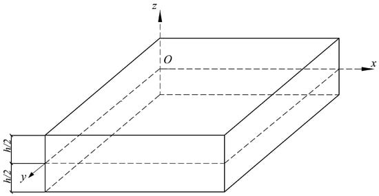
Figure 1. The adopted coordinate system.

The proposed methodology is based on the ideas presented in refs. [31,32]. Compared to work [31], the approach proposed here allows for different heat exchange conditions on surfaces to be taken into account. Unlike the approach given in work [32], information on temperatures at all points along the thickness of the slab is not required. That is, in terms of the level of simplification, the proposed approach occupies an intermediate position between works [31,32]. The following hypotheses are used:

• The temperature in the slab is a function of the coordinate $z$ only; the boundary effects are neglected. This hypothesis is confirmed by the results of three-dimensional finite element analysis of temperature fields: with the exception of the edges, the temperature distribution in the foundation slabs is one-dimensional (Figure 2).
  

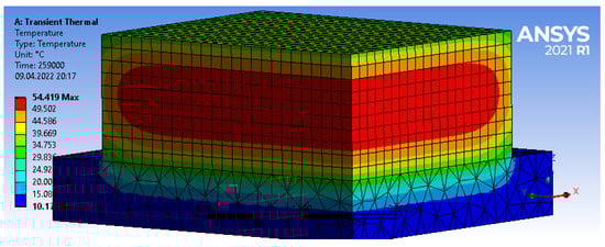  Figure 2. Character of the temperature distribution in a massive monolithic foundation slab obtained by finite element analysis.

2.

Stresses ${\sigma }_z$, ${\tau }_{xy}$, ${\tau }_{xz}$, ${\tau }_{yz}$ and the corresponding deformations are also neglected.

These hypotheses are also based on the results of three-dimensional finite element analysis. Except at the edges, the indicated stress and strain components are close to zero (Figure 3, Figure 4, Figure 5 and Figure 6).

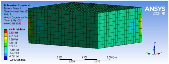
Figure 3. Character of stress ${\sigma }_z$ distribution in a massive foundation slab.

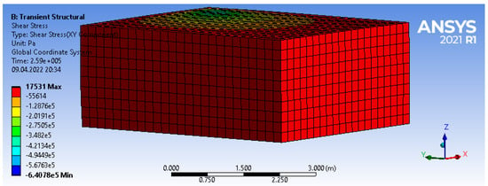
Figure 4. Character of stress ${\tau }_{xy}$ distribution in a massive foundation slab.

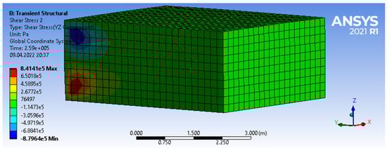
Figure 5. Character of stress ${\tau }_{yz}$ distribution in a massive foundation slab.

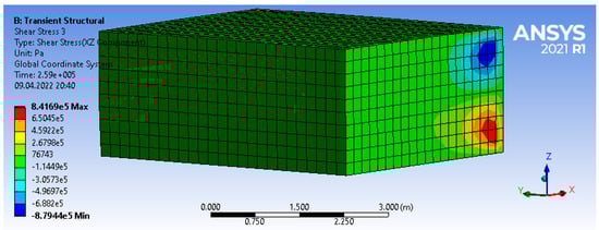
Figure 6. Character of stress ${\tau }_{xz}$ distribution in a massive foundation slab.

3.

Stresses ${\sigma }_x$ and ${\sigma }_y$ are taken to be equal to each other (${\sigma }_x={\sigma }_y=\sigma$), and it is assumed that they depend only on the coordinate $z$. This hypothesis is also based on the results of three-dimensional finite element analysis (Figure 7).

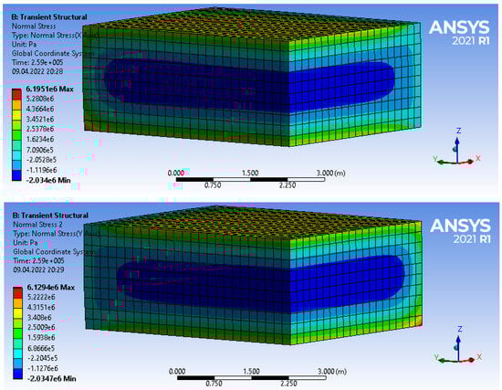Figure 7. The character of the distribution for stresses ${\sigma }_x$ (top) and ${\sigma }_y$ (bottom).

4.

Total deformations ${\epsilon }_x$ and ${\epsilon }_y$ are also taken to be equal to each other and constant in thickness (${\epsilon }_x={\epsilon }_y=\epsilon$). This hypothesis follows from hypotheses 2 and 3.

5.

The concrete modulus of elasticity is assumed to depend only on time; its change across the thickness of the slab is neglected.

Hypothesis 5 was previously used in ref. [31]. Its use allowed us to express thermal stresses through the temperature difference between the center and surface of the structure.

The increments of deformations in concrete over time $\Delta t$ based on hypothesis 2 can be written as:

$$\Delta {\epsilon }_x=\Delta \epsilon ={\displaystyle \frac{1}{E}}\left(\Delta {\sigma }_x-\nu \Delta {\sigma }_y\right)+\alpha \Delta T={\displaystyle \frac{1-\nu }{E}}\Delta \sigma +\alpha \Delta T,$$

(2)

where $E$ is the modulus of elasticity of concrete, $\nu =0.2$ is the Poisson’s ratio of concrete, $\alpha$ is the coefficient of linear thermal expansion of concrete, and $\Delta T=T_t-T_{t-\Delta t}$ is the change in temperature at the point under consideration over time $\Delta t$.

Expressing the stress increment $\Delta \sigma$ from (2) leads to the equation:

$$\Delta \sigma ={\displaystyle \frac{E}{1-\nu }}\left(\Delta \epsilon -\alpha (T_t-T_{t-\Delta t})\right).$$

(3)

Since there are no effects on the slab other than temperature during the construction stage, the increase in axial forces over time $\Delta t$ can be taken to be zero:

$$\Delta N=\underset{-h/2}{\overset{h/2}{\int }}\Delta \sigma dz=0.$$

(4)

Substituting (3) into (4) leads to the equality:

$$\Delta \epsilon \cdot h-\alpha \left(\underset{-{\displaystyle \frac{h}{2}}}{\overset{{\displaystyle \frac{h}{2}}}{\int }}{T}_t\left(z\right)dz-\underset{-{\displaystyle \frac{h}{2}}}{\overset{{\displaystyle \frac{h}{2}}}{\int }}{T}_{t-\Delta t}\left(z\right)dz\right)=0.$$

(5)

To calculate integrals of the type ${\int }_{-h/2}^{h/2}T\left(z\right)dz$ over the slab thickness, the Simpson’s formula is used:

$$\underset{-h/2}{\overset{h/2}{\int }}T\left(z\right)dz={\displaystyle \frac{h}{6}}\left(T^{bot}+4T^{mid}+T^{up}\right),$$

(6)

where $T^{bot}$ is the temperature at the lower surface of the slab, $T^{mid}$ is the temperature in the middle of the thickness, and $T^{up}$ is the temperature at the upper surface of the slab.

Taking into account (6), the expression for the increment of deformation $\Delta \epsilon$ will take the form:

$$\Delta \epsilon ={\displaystyle \frac{\alpha }{6}}\left[\left(T_t^{bot}-T_{t-\Delta t}^{bot} \right)+4\left(T_t^{mid}-T_{t-\Delta t}^{mid} \right)+\left(T_t^{up}-T_{t-\Delta t}^{up} \right)\right].$$

(7)

Substitution of (7) into (3) gives the expressions for the stress increments at three characteristic points (at the lower surface, in the middle of the thickness, and at the upper surface):

$$\Delta {\sigma }_{bot}={\displaystyle \frac{E\alpha \left(-5\left(T_t^{bot}-T_{t-\Delta t}^{bot}\right)+4\left(T_t^{mid}-T_{t-\Delta t}^{mid} \right)+\left(T_t^{up}-T_{t-\Delta t}^{up} \right)\right)}{6\left(1-\nu \right)}},$$

(8)

$$\Delta {\sigma }_{mid}={\displaystyle \frac{E\alpha \left(\left(T_t^{bot}-T_{t-\Delta t}^{bot}\right)-2\left(T_t^{mid}-T_{t-\Delta t}^{mid} \right)+\left(T_t^{up}-T_{t-\Delta t}^{up} \right)\right)}{6\left(1-\nu \right)}},$$

(9)

$$\Delta {\sigma }_{up}={\displaystyle \frac{E\alpha \left(\left(T_t^{bot}-T_{t-\Delta t}^{bot}\right)+4\left(T_t^{mid}-T_{t-\Delta t}^{mid} \right)-5\left(T_t^{up}-T_{t-\Delta t}^{up} \right)\right)}{6\left(1-\nu \right)}}.$$

(10)

The resulting Formulas (8)–(10) are very easy to use for practitioners and require only data on temperatures at three points of the slab (bottom, middle, top) at different moments in time, as well as data on the change in the modulus of elasticity of concrete over time. Since the formulas are written in increments, the more time points, the more accurate the result. Calculations using these formulas can be implemented in spreadsheets, for example, MS Excel.

In the particular case where the heat exchange conditions on the upper and lower surfaces are the same ($T^{bot}=T^{up}=T^{surf}$), Formulas (8)–(10) will take the form:

$$\begin{gathered} \Delta {\sigma }_{mid}={\displaystyle \frac{E\alpha \left(\left(T_t^{surf}-T_{t-\Delta t}^{surf}\right)-\left(T_t^{mid}-T_{t-\Delta t}^{mid} \right)\right)}{3\left(1-\nu \right)}}; \\ \Delta {\sigma }_{surf}={\displaystyle \frac{2E\alpha \left(\left(T_t^{mid}-T_{t-\Delta t}^{mid}\right)-\left(T_t^{surf}-T_{t-\Delta t}^{surf} \right)\right)}{3\left(1-\nu \right)}}=-2\Delta {\sigma }_{mid}. \end{gathered}$$

(11)

Formulas (11) coincide with the formulas obtained in ref. [31].

By introducing the notation $k={\displaystyle \frac{2}{3(1-\nu )}}=0.833$, the following formula can be obtained:

$$\Delta {\sigma }_{surf}=k\alpha E\left[\left(T_t^{mid}-T_t^{surf}\right)-\left(T_{t-\Delta t}^{mid}-T_{t-\Delta t}^{surf}\right)\right].$$

(12)

Formula (12) differs from Formula (1) only by the multiplier $(1+\phi )$, which takes into account creep, and also by the fact that Formula (12) is written in increments, which is more correct for calculations of structures with a time-varying modulus of elasticity.

It should also be noted that if the average value between $T^{up}$ and $T^{bot}$ as $T^{surf}$ as taken in (11), then the formula for the middle of the thickness will coincide with formula (9). However, for the upper and lower surfaces, there will be significant differences from Formulas (8) and (10):

$$\begin{gathered} \Delta {\sigma }_{surf}={\displaystyle \frac{2E\alpha \left(\left(T_t^{mid}-T_{t-\Delta t}^{mid}\right)-\frac{1}{2}\left(T_t^{up}-T_{t-\Delta t}^{up} \right)-\frac{1}{2}\left(T_t^{bot}-T_{t-\Delta t}^{bot} \right)\right)}{3\left(1-\nu \right)}} \\ ={\displaystyle \frac{E\alpha \left(4\left(T_t^{mid}-T_{t-\Delta t}^{mid}\right)-2\left(T_t^{up}-T_{t-\Delta t}^{up} \right)-2\left(T_t^{bot}-T_{t-\Delta t}^{bot} \right)\right)}{6\left(1-\nu \right)}}. \end{gathered}$$

(13)

From Formula (13), it is easy to see that when substituting the average between $T^{up}$ and $T^{bot}$ instead of $T^{surf}$ into Formula (11), the average value of the stress increment on the surface will be obtained:

$$\Delta {\sigma }_{surf}={\displaystyle \frac{\Delta {\sigma }_{up}+\Delta {\sigma }_{bot}}{2}}.$$

(14)

2.2. Formulation of the Test Problem

To test the obtained Formulas (8)–(10), the first stage was a comparison with the results of the experiment to determine the temperature stresses, as well as the results of the calculation by the finite element method in a three-dimensional formulation for a massive foundation slab, given in the work [33]. The characteristics of the slab under consideration are given in Table 1.

Table 1. Characteristics of the slab under consideration.

Cement consumption, kg/m3	240
28-day compressive strength of concrete, MPa	34.2
28-day tensile strength of concrete, MPa	1.83
$\mathrm{Slab} \mathrm{dimensions} a\times b\times h$, m	26.5 × 41.5 × 2
Thickness of the soil massif under the foundation slab in the finite element calculation, m	10
$\mathrm{Concrete} \mathrm{density} \rho$, kg/m3	2.349
$\mathrm{Specific} \mathrm{heat} \mathrm{capacity} \mathrm{of} \mathrm{concrete} c$, kJ/(kg∙°C)	0.979
Concrete modulus of elasticity at the age of 28 days, GPa	34.4
$\mathrm{Concrete} \mathrm{coefficient} \mathrm{of} \mathrm{linear} \mathrm{thermal} \mathrm{expansion} \alpha$, 1/°C	1.2 × 10−5
$\mathrm{Thermal} \mathrm{conductivity} \mathrm{coefficient} \mathrm{of} \mathrm{concrete} \lambda$, W/(m∙°C)	2.67
$\mathrm{Density} \mathrm{of} \mathrm{soil} {\rho }_g$, t/m3	2.070
$\mathrm{Specific} \mathrm{heat} \mathrm{capacity} \mathrm{of} \mathrm{the} \mathrm{soil} c_g,$ kJ/(kg∙°C)	1.039
$\mathrm{Thermal} \mathrm{conductivity} \mathrm{coefficient} \mathrm{of} \mathrm{the} \mathrm{soil} {\lambda }_g$, W/(m∙°C)	1.4
Initial temperature of concrete mix, °C	24
$\mathrm{Initial} \mathrm{soil} \mathrm{temperature} T_{soil}$, °C	16
$\mathrm{Heat} \mathrm{transfer} \mathrm{coefficient} \mathrm{on} \mathrm{the} \mathrm{upper} \mathrm{surface} h_{up}$, W/(m2∙°C)	30

The temperature field was calculated in a one-dimensional formulation using the method given in ref. [34] using the differential equation:

$$\lambda {\displaystyle \frac{{\partial }^{2}T}{\partial z^2}}+W=\rho c{\displaystyle \frac{\partial T}{\partial t}},$$

(15)

where $T$ is the temperature, $W={\displaystyle \frac{\partial Q}{\partial t}}$ is the specific power of internal heat sources (W/m³).

On the upper surface of the slab, the boundary conditions for convective heat exchange with the environment were adopted:

$$\lambda {\displaystyle \frac{\partial T}{\partial z}}+h_{up}\left(T-T_{amb}\right)=0,$$

(16)

where $T_{amb}$ is the ambient temperature.

At the lowest points of the soil massif, the temperature was taken to be equal to $T_{soil}$.

The value $W$ at the current moment in time was assumed to depend on the temperature of the concrete. To take into account the dependence of the heat release intensity on temperature, the formula of S.V. Aleksandrovsky [35] was used:

$$W\left(t\right)=\rho c\omega \left(t\right)\cdot T\left(t\right).$$

(17)

The function $\omega \left(t\right)$ in Equation (14) has the form:

$$\omega \left(t\right)={\displaystyle \frac{B{(\theta }_{\infty }-{\theta }_0)}{({\theta }_{\infty }+{\theta }_0[\exp \left(B{\theta }_{\infty }t\right)-1\left]\right)}},$$

(18)

where ${\theta }_0=20 °\mathrm{C}$ is the initial temperature of the adiabatic heat release process in laboratory tests, $B$ is a constant characterizing the intensity of heat release, and ${\theta }_{\infty }$ is the maximum temperature in adiabatic tests, which is calculated using the formula:

$${\theta }_{\infty }={\theta }_0+{\displaystyle \frac{qC}{\rho c}},$$

(19)

where $C$ is the cement content in concrete (kg/m³), and $q$ is the total amount of heat released by 1 kg of cement during the entire hydration period.

Constants $q$ and $B$ in the calculation were taken as equal to: q = 3.2 × 10⁵ J/kg, B = 7 × 10⁻⁴ 1/(°C∙h). These values of constants were adopted on the basis of literature data [35] on the average heat release of concretes with similar composition.

When calculating temperature stresses, the modulus of elasticity of concrete was determined using the formula [33]:

$$E\left(t_{eq}\right)={\alpha }_1\exp \left[-{\left({\displaystyle \frac{{\tau }_1}{t_{eq}}}\right)}^{{\beta }_1}\right]+{\alpha }_2\exp \left[-{\left({\displaystyle \frac{{\tau }_2}{t_{eq}}}\right)}^{{\beta }_2}\right],$$

(20)

where $t_{eq}$ is the equivalent age of concrete, taking into account the acceleration of concrete strength gain at elevated temperatures, which is determined by the formula:

$$t_{eq}=\underset{0}{\overset{t}{\int }}\exp \left[-{\displaystyle \frac{E_a}{R}}\left({\displaystyle \frac{1}{T\left(\tau \right)+273}}-{\displaystyle \frac{1}{T_{ref}+273}}\right)\right]d\tau ,$$

(21)

where $R$ is the universal gas constant, $E_a$ is the activation energy, and $T_{ref}=20 °\mathrm{C}$ is the standard temperature.

The constants included in Equations (18) and (19) are given in Table 2.

Table 2. Constants included in Equations (18) and (19).

Quantity	Units of Measurement	Value
${\alpha }_1$	GPa	15
${\alpha }_2$	GPa	20
${\beta }_1$	-	1.5
${\beta }_2$	-	1.5
${\tau }_1$	day	2
${\tau }_2$	day	4
${\displaystyle \frac{E_a}{R}}$	J/K	4630

3. Results

Figure 8 shows a comparison of experimental and calculated temperatures for the slab’s bottom surface, midsection, and top surface. The calculated maximum temperature at the midsection was 43.9 °C, which is only 0.9% different from the experimental maximum (44.3 °C). The maximum calculated temperature at the bottom surface was 36.3 °C, which is only 0.1 °C different from the experimental value. A noticeable discrepancy is observed at some points in time between the temperatures at the top surface, which can be explained by additional heating from solar radiation.

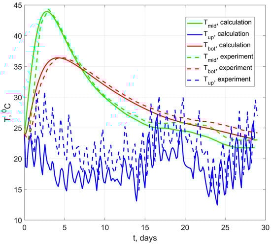
Figure 8. Comparison of experimental temperatures with calculated ones.

Figure 9 shows a comparison of the stress calculations results in the middle of the thickness using Formula (9) with the experimental data and the results of finite element modeling presented in ref. [33]. For comparison, the results using Formula (1) are also provided. It should be immediately noted that the 3D finite element modeling results and the experimental results presented in ref. [33] have only a qualitative coincidence. After 16 days, a drop in stress to approximately zero is observed on the experimental curve, which indicates the possible formation of a crack or failure of the sensor. At the time of 15.75 days, the maximum tensile stress in the experiment is 0.7 MPa, and according to the calculation results of the authors of ref. [33], the stress value at this time is 2.45 MPa.

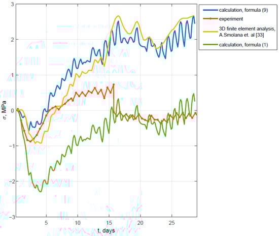
Figure 9. Comparison of calculation results with solutions of other authors and experimental data.

At the same time, our proposed method provides good agreement with the results of three-dimensional finite element analysis. The tensile stress at the final time of 28.5 days using Formula (9) is 2.67 MPa, while in the three-dimensional finite element analysis it is equal to 2.68 MPa.

It should be noted that Formula (1) does not allow even for a qualitative description of the stress–strain state. As noted earlier, this is because Formula (1) does not take into account the entire history of changes in the concrete’s elastic modulus up to the point in time under consideration.

4. Discussion

First, the reasons for the discrepancy between the calculated results and the experimental data should be discussed. In ref. [36], it was previously demonstrated that stresses in hardening massive monolithic structures depend significantly on how the concrete modulus of elasticity changes over time in the early period up to 24 h. At a very early age (several hours), concrete is an unstable substance that, after setting, quite abruptly acquires the properties of a solid, and the moment of this transition can vary significantly. The resulting stresses depend significantly on what is taken as the initial moment of time when the modulus of elasticity of concrete becomes nonzero. Also, concrete at an early age is characterized by rapid creep, which has been little studied. Failure to account for the rapid creep at an early age leads to an overestimation of the calculated stresses, which is precisely what is observed in the problem under consideration.

Accounting for rapid creep and determining the induction period after which concrete can be treated as a solid, as well as determining stresses in it using the equations of elasticity theory, will be the subject of our further research. If data on rapid creep are available, it can be accounted for by underestimating the concrete’s deformation modulus or by introducing a factor $(1+\phi )$ into Formulas (8)–(10), as in Formula (1). According to our preliminary data, taking creep into account can lead to a reduction in stresses by up to 1.6 times.

In the calculation example considered, in addition to rapid creep, autogenous shrinkage deformations were also not taken into account. Given the availability of data on concrete shrinkage at an early age, accounting for this deformation does not present significant difficulties. The most common approach to accounting for shrinkage deformations is to consider them as an equivalent temperature effect [37,38]. The calculated temperature values $T_{calc}$ can be calculated using the formula:

$$T_{calc}=T_{fact}-{\displaystyle \frac{{\epsilon }_{sh}}{\alpha }},$$

(22)

where $T_{fact}$ are the actual temperature values, ${\epsilon }_{sh}$ are the absolute values of shrinkage deformations.

Experiments show that the maximum value of autogenous shrinkage deformation of concrete at the age of 28 days can vary in the range of approximately 20 × 10⁻⁶ to 80 × 10⁻⁶ [39,40]. At a maximum value of 80 × 10⁻⁶ and $\alpha ={10}^{-5} 1/°\mathrm{C}$ the ratio ${\epsilon }_{sh}/\alpha$ is equal to $8 °\mathrm{C}$. With a temperature range in a massive structure from 20 to 80 $°\mathrm{C}$, the contribution of the term ${\epsilon }_{sh}/\alpha$ will be from 40% to 10%. However, it should be noted that the magnitude of stress is not affected by the shrinkage deformation itself, but by the uneven distribution of deformations across the thickness of the slab, and the final contribution of shrinkage can only be determined by modeling. Also, at an early age of 3–5 days, when the risk of early cracking is the greatest, the values of shrinkage deformations will be significantly less than 80 × 10⁻⁶.

Next, it is necessary to discuss another limitation of the approach proposed in this article. When integrating over the slab thickness, the Simpson’s formula was used, which yields an accurate result only when the function varies linearly or quadratically. A square parabola $a{T}^2+bT+c$ is an exact solution of the heat conductivity Equation (15) in the case when ${\displaystyle \frac{\partial T}{\partial \tau }}\to 0$, since the power of heat release $W$ is constant across the thickness of the slab. When the term $\rho c{\displaystyle \frac{\partial T}{\partial t}}$ is small compared to $W$, the temperature distribution will also be close to parabolic. This condition is violated at the initial moments of time, when the temperature changes quite quickly.

Figure 10 shows graphs of the temperature distribution across the slab thickness at various points in time. This figure clearly shows that, at initial points in time, the curves $T\left(z\right)$ deviate significantly from parabolic. There are near-surface layers where the main temperature gradient occurs, and a structural core where the temperature remains virtually constant along the z-coordinate. Subsequently, the temperature distribution becomes more parabolic over time. This may explain why Figure 9 shows a greater deviation between the calculation results obtained using our proposed method and the results of the 3D finite element analysis at initial points in time. The size of the core layer, in which the temperature conditions are close to adiabatic, depends on the thickness of the slab: as it increases, the thickness of the core layer also increases, and Formulas (8)–(10) can give larger errors.

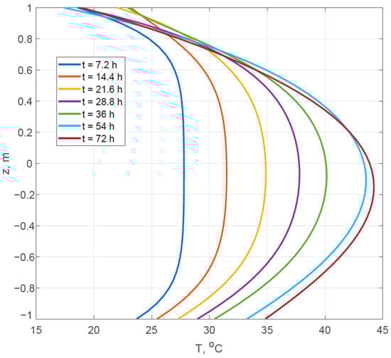
Figure 10. Temperature distribution across the slab thickness at different points in time.

To assess the limits of applicability of Formulas (8)–(10), a series of finite element calculations were performed for slab thicknesses of 1 m, 1.5 m, 2 m, and 2.5 m. For the sake of simplicity, daily changes in the ambient temperature were not taken into account; the value $T_{amb}$ was taken as constant and equal to 17.5 °C. The remaining initial data were taken as in the test problem.

Figure 11, Figure 12 and Figure 13 show graphs of stress changes over time in the middle of the thickness at the lower and upper surfaces. Dashed lines correspond to the calculation results using Formulas (8)–(10), and solid lines correspond to those obtained using the finite element method.

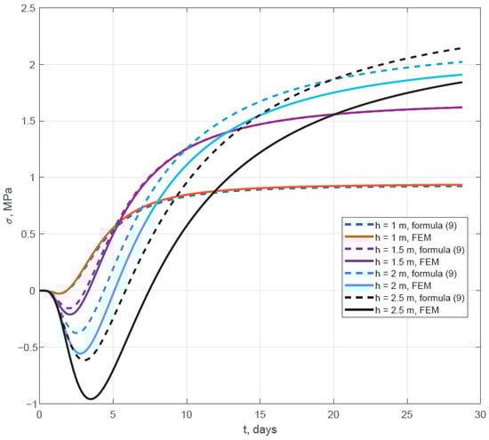
Figure 11. Change in stresses in the middle of the thickness over time.

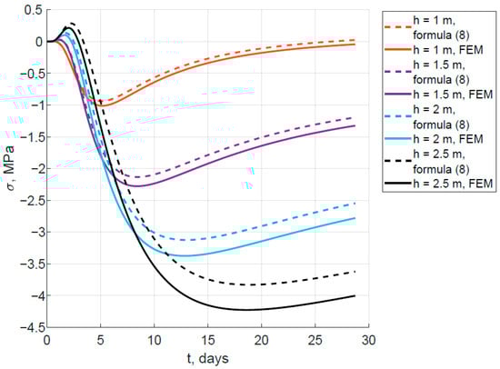
Figure 12. Change in stress at the lower surface over time.

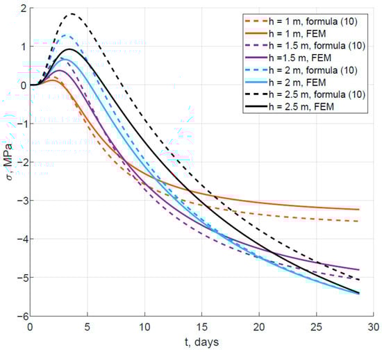
Figure 13. Change in stress at the upper surface over time.

From Figure 11, Figure 12 and Figure 13, it is evident that with increasing slab thickness, the error in determining stresses using Formulas (8)–(10) generally tends to increase. A comparison of the maximum absolute stress values for three calculation points with different slab thicknesses is given in Table 3. For slab thicknesses up to 2 m, the error in determining stresses does not exceed 10%.

Table 3. Comparison of maximum absolute stress values.

		Stresses, kPa		Error, %
		FEM	Simplified Methodology
h = 1 m	bottom	1012	939	7.2
	middle	935	879	6.0
	top	3235	3540	9.4
h = 1.5 m	bottom	2278	2134	6.3
	middle	1620	1562	3.6
	top	4802	5051	5.2
h = 2 m	bottom	3375	3124	7.4
	middle	1909	1994	4.5
	top	5432	5430	0.04
h = 2.5 m	bottom	4226	3830	9.4
	middle	1842	2171	17.9
	top	5404	5062	6.3

Also, to test the proposed method, a series of 125 finite element calculations were performed with different input parameter values. The thickness of the slab varied from 1 to 2 m in steps of 0.25 m. The heat transfer coefficient on the upper surface varied from 5 to 25 W/(m²∙°C) in increments of 5 W/(m²∙°C). The ambient temperature varied from 5 to 25 °C in steps of 5 °C. The initial temperature of the concrete mixture was assumed to be equal to the ambient temperature, but no more than 20 °C. The same was assumed for the initial soil temperature. The remaining parameters, including the heat release function and the dependence of the modulus of elasticity of concrete on time, were taken as before.

For each variant, the maximum value of tensile stresses was determined. In Figure 14, the abscissa axis shows the values ${\sigma }_{FEM}$ obtained using the finite element method, and the ordinate axis shows the values ${\sigma }_s$ obtained using the proposed simplified method. Most of the points lie at a small distance from the straight line ${\sigma }_s={\sigma }_{FEM}$. The deviation is observed in the zone of high stresses, which generally exceed the tensile strength of concrete and are unacceptable. The highest stress levels are observed when three factors are simultaneously at work: large slab thickness, high surface heat transfer coefficient and high ambient temperature. In this case, the simplified method predicts stresses with a certain safety margin compared to the FEM. The average value of the ratio ${\sigma }_s/{\sigma }_{FEM}$ was 1.03; the minimum was 0.95, the maximum was 1.39 and the standard deviation was 0.1.

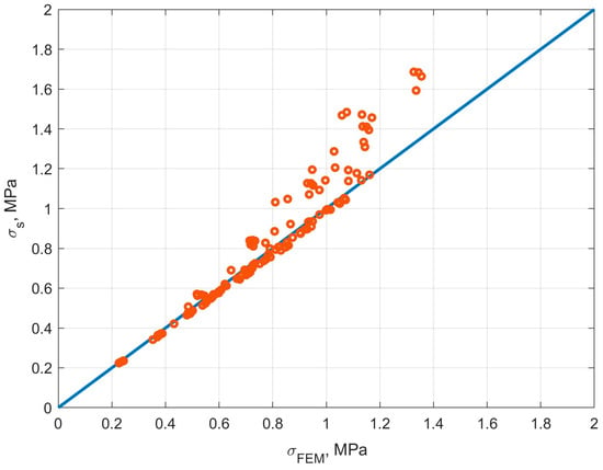
Figure 14. Comparison of the calculation results using a simplified method with the results of finite element modeling.

5. Conclusions

Formulas have been obtained for determining thermal stresses during the construction of massive monolithic foundation slabs based on temperatures at three points: the bottom surface, the center of the slab, and the top surface. Unlike the existing approach, which expresses stresses through the temperature difference between the center and surface of the structure, our proposed approach allows for different heat transfer conditions at the top and bottom surfaces of the foundation slab. The proposed approach has been validated by comparison with experimental data and the results of a three-dimensional finite element analysis presented in A. Smolana et al. [33]. Good agreement with the results of the three-dimensional finite element analysis was established; the difference in the magnitude of the maximum tensile stresses was only 0.01 MPa. Only qualitative agreement with the experimental data was observed, which can be explained by insufficient data on the change in the elastic modulus of concrete over time in the early period up to 1 day, as well as by not taking into account the rapid creep of concrete. Our further research will be aimed at refining the data on changes in the concrete deformation characteristics at an early age, as well as studying the rapid creep that manifests itself during strength gain.

To assess the applicability limits of the obtained formulas, a series of calculations were performed for foundation slab thicknesses ranging from 1 to 2.5 m. Since Simpson’s formula was used to integrate the temperature change function across the slab thickness, our proposed formulas provide accurate results only if the temperature distribution follows the law of a square parabola. During the initial period of curing, the temperature distribution across the thickness deviates from parabolic: there are near-surface layers where the greatest temperature gradient occurs, and a core layer where temperature conditions are close to adiabatic, and the temperature is virtually constant. Over time, the temperature distribution becomes closer to parabolic. The size of the core layer increases with increasing slab thickness, and accordingly, the error in our proposed formulas tends to increase with increasing thickness. The method is recommended for use with slab thicknesses of no more than 2 m. A series of finite element calculations for different values of input parameters showed that for a slab thickness of up to 2 m, the average error in determining the maximum tensile stresses compared to FEM is 3%, and the maximum error is 39%. The greatest error is observed at high stress levels exceeding the tensile strength of concrete, but, in this case, the simplified method predicts stresses with a reserve compared to FEM.

The proposed methodology can be integrated into real-time monitoring systems for massive reinforced concrete structures, such as Maturix [41], Giatec SmartRock [42,43], ConMonity [44], etc., for real-time estimation of early cracking risk. The implementation of real-time stress assessment will allow on-site decisions to be made on the timing of opening structures or on additional insulation of surfaces when stresses approach dangerous levels. This will also eliminate the need for expensive strain gauges, which must be able to adjust readings based on temperature.

Compared to the FEM, the proposed approach does not require information on temperatures at all nodes for calculating stresses and allows for the stress prediction to be adjusted if the actual temperatures in the structure deviate from the precalculated ones.

References

- Mihashi, H.; Leite, J.P.B. State-of-the-Art Report on Control of Cracking in Early Age Concrete. J. Adv. Concr. Technol. 2004, 2, 141–154. [Google Scholar] [CrossRef]
- Safiuddin, M.; Kaish, A.B.M.; Woon, C.-O.; Raman, S.N. Early-Age Cracking in Concrete: Causes, Consequences, Remedial Measures, and Recommendations. Appl. Sci. 2018, 8, 1730. [Google Scholar] [CrossRef]
- Waller, V.; d’Aloïa, L.; Cussigh, F.; Lecrux, S. Using the Maturity Method in Concrete Cracking Control at Early Ages. Cem. Concr. Compos. 2004, 26, 589–599. [Google Scholar] [CrossRef]
- Wu, L.; Farzadnia, N.; Shi, C.; Zhang, Z.; Wang, H. Autogenous Shrinkage of High Performance Concrete: A Review. Constr. Build. Mater. 2017, 149, 62–75. [Google Scholar] [CrossRef]
- Zhang, J.; Han, Y.D.; Zhang, J.J. Evaluation of Shrinkage Induced Cracking in Concrete with Impact of Internal Curing and Water to Cement Ratio. J. Adv. Concr. Technol. 2016, 14, 324–334. [Google Scholar] [CrossRef]
- Mazzoli, A.; Monosi, S.; Plescia, E.S. Evaluation of the Early-Age-Shrinkage of Fiber Reinforced Concrete (FRC) Using Image Analysis Methods. Constr. Build. Mater. 2015, 101, 596–601. [Google Scholar] [CrossRef]
- Do, T.A.; Tia, M.; Nguyen, T.H.; Nguyen, T.T.; Nguyen, T.C. Assessment of Temperature Evolution and Early-Age Thermal Cracking Risk in Segmental High-Strength Concrete Box Girder Diaphragms. KSCE J. Civ. Eng. 2022, 26, 166–182. [Google Scholar] [CrossRef]
- Kuriakose, B.; Rao, B.N.; Dodagoudar, G.R. Early-Age Temperature Distribution in a Massive Concrete Foundation. Procedia Technol. 2016, 25, 107–114. [Google Scholar] [CrossRef]
- Pulkit, U.; Das Adhikary, S. Effect of micro-structural changes on concrete properties at elevated temperature: Current knowledge and outlook. Struct. Concr. J. Fib 2022, 23, 1995–2014. [Google Scholar] [CrossRef]
- Alos Shepherd, D.; Dehn, F. Experimental Study into the Mechanical Properties of Plastic Concrete: Compressive Strength Development over Time, Tensile Strength and Elastic Modulus. Case Stud. Constr. Mater. 2023, 19, e02521. [Google Scholar] [CrossRef]
- Ivashenko, Y.; Ferder, A. Experimental Studies on the Impacts of Strain and Loading Modes on the Formation of Concrete “Stress-Strain” Relations. Constr. Build. Mater. 2019, 209, 234–239. [Google Scholar] [CrossRef]
- Xu, J.; Shen, Z.; Yang, S.; Xie, X.; Yang, Z. Finite Element Simulation of Prevention Thermal Cracking in Mass Concrete. Int. J. Comput. Sci. Math. 2019, 10, 327–339. [Google Scholar] [CrossRef]
- Coelho, N.d.A.; Pedroso, L.J.; Rêgo, J.H.d.S.; Nepomuceno, A.A. Use of ANSYS for Thermal Analysis in Mass Concrete. J. Civ. Eng. Archit. 2014, 8, 860–868. [Google Scholar] [CrossRef]
- Reutov, Y.Y.; Gobov, Y.L.; Loskutov, V.E. Feasibilities of Using the ELCUT Software for Calculations in Nondestructive Testing. Russ. J. Nondestruct. Test. 2002, 38, 425–430. [Google Scholar] [CrossRef]
- Shea, G.; Chen, Y.; Xu, S.; Zhang, T.; Liange, Y. Simulation Research of Foundation Excavation Retaining and Protecting Optimization Based on Midas Structural Analysis Technology. Acad. J. Eng. Technol. Sci. 2022, 5, 13–23. [Google Scholar] [CrossRef]
- Sheng, X.; Xiao, S.; Zheng, W.; Sun, H.; Yang, Y.; Ma, K. Experimental and Finite Element Investigations on Hydration Heat and Early Cracks in Massive Concrete Piers. Case Stud. Constr. Mater. 2023, 18, e01926. [Google Scholar] [CrossRef]
- Xie, Y.; Du, W.; Xu, Y.; Peng, B.; Qian, C. Temperature Field Evolution of Mass Concrete: From Hydration Dynamics, Finite Element Models to Real Concrete Structure. J. Build. Eng. 2023, 65, 105699. [Google Scholar] [CrossRef]
- Chen, H.; Liu, D. Numerical Simulations of Multiple Cracks in Concrete Face Rockfill Dams Coupled Multi-Factor during Construction. Case Stud. Constr. Mater. 2025, 22, e04609. [Google Scholar] [CrossRef]
- Zhang, F.; Liao, L.; Tian, F. Research on Temperature Control Techniques for Mass Concrete in the Pile Cap of the West Tower of Shiziyang Bridge. J. Eng. Appl. Sci. 2025, 72, 138. [Google Scholar] [CrossRef]
- Cao, W.; Liang, N.; Peng, L.; Zhong, Z.; Zhou, X.; Suliman, L. Study the Influence of Basalt Fiber on Temperature Cracks in Mass Concrete Pile Cap. Structures 2025, 80, 109851. [Google Scholar] [CrossRef]
- Yang, F.; Zeng, X.; Xia, Q.; Yang, L.; Cai, H.; Cheng, C. Early Detection and Analysis of Cavity Defects in Concrete Columns Based on Infrared Thermography and Finite Element Analysis. Materials 2025, 18, 1686. [Google Scholar] [CrossRef] [PubMed]
- Zhou, J.; Li, X.; Wang, Z.; Wang, Y.; Yan, C.; Jin, H. Numerical Analysis of Temperature Stress Generated by Hydration Heat in Massive Concrete Pier. Period. Polytech. Civ. Eng. 2025, 69, 461–469. [Google Scholar] [CrossRef]
- Wang, T.; Cai, J.; Feng, Q.; Jia, W.; He, Y. Experimental Study and Numerical Analysis of Hydration Heat Effect on Precast Prestressed Concrete Box Girder. Buildings 2025, 15, 859. [Google Scholar] [CrossRef]
- Smolana, A.; Klemczak, B.; Azenha, M.; Schlicke, D. Early age cracking risk in a massive concrete foundation slab: Comparison of analytical and numerical prediction models with on-site measurements. Constr. Build. Mater. 2021, 301, 124135. [Google Scholar] [CrossRef]
- Li, X.; Yu, Z.; Chen, K.; Deng, C.; Yu, F. Investigation of Temperature Development and Cracking Control Strategies of Mass Concrete: A Field Monitoring Case Study. Case Stud. Constr. Mater. 2023, 18, e02144. [Google Scholar] [CrossRef]
- Mehta, P.K.; Monteiro, P.J.M. Concrete: Microstructure, Properties, and Materials; McGraw-Hill: New York, NY, USA, 2006. [Google Scholar] [CrossRef]
- Liu, L.; Zhao, S.; Xin, J.; Wang, Z. Simplified Analysis of Thermal Cracks in Low-Heat Portland Cement Concrete. Adv. Civ. Eng. 2022, 2022, 7630568. [Google Scholar] [CrossRef]
- Aniskin, N.A.; Nguyen, T.C. Predictive Model of Temperature Regimes of a Concrete Gravity Dam during Construction: Reducing Cracking Risks. Buildings 2023, 13, 1954. [Google Scholar] [CrossRef]
- Nguyen, C.T.; Luu, X.B. Reducing Temperature Difference in Mass Concrete by Surface Insulation. Mag. Civ. Eng. 2019, 88, 70–79. [Google Scholar] [CrossRef]
- Van Lam, T.; Nguen, C.C.; Bulgakov, B.I.; Anh, P.N. Composition Calculation and Cracking Estimation of Concrete at Early Ages. Mag. Civ. Eng. 2018, 82, 13. [Google Scholar] [CrossRef]
- Chepurnenko, A.; Turina, V. Simplified Method for Determining Thermal Stresses during the Construction of Massive Monolithic Foundation Slabs. CivilEng 2023, 4, 740–752. [Google Scholar] [CrossRef]
- Chepurnenko, A.; Nesvetaev, G.; Koryanova, Y.; Yazyev, B. Simplified Model for Determining the Stress-Strain State in Massive Monolithic Foundation Slabs during Construction. Int. J. Comput. Civ. Struct. Eng. 2022, 18, 126–136. [Google Scholar] [CrossRef]
- Smolana, A.; Klemczak, B.; Azenha, M.; Schlicke, D. Thermo-Mechanical Analysis of Mass Concrete Foundation Slabs at Early Age—Essential Aspects and Experiences from the FE Modelling. Materials 2022, 15, 1815. [Google Scholar] [CrossRef] [PubMed]
- Chepurnenko, A.; Nesvetaev, G.; Koryanova, Y. Modeling Non-Stationary Temperature Fields when Constructing Mass Cast-In-Situ Reinforced-Concrete Foundation Slabs. Archit. Eng. 2022, 7, 66–78. [Google Scholar] [CrossRef]
- Aleksandrovsky, S.V. Calculation of Concrete and Reinforced Concrete Structures for Changes in Temperature and Humidity Taking into Account Concrete Creep; NIIZHB: Moscow, Russia, 2004; Available online: https://science.totalarch.com/book/3164.rar (accessed on 3 November 2025).
- Tyurina, V.; Chepurnenko, A.; Akopyan, V. Prediction of Thermal Cracking During Construction of Massive Monolithic Structures. Appl. Sci. 2025, 15, 1499. [Google Scholar] [CrossRef]
- Zheng, X.; Zhang, J. Finite Element Simulation for Bending Behavior of Steel-ECC Composite Slab Considering Shrinkage, Creep and Cracking. Constr. Build. Mater. 2021, 282, 122643. [Google Scholar] [CrossRef]
- Zhu, J.; Wang, C.; Yang, Y.; Wang, Y. Hygro-Thermal–Mechanical Coupling Analysis for Early Shrinkage of Cast In Situ Concrete Slabs of Composite Beams: Theory and Experiment. Constr. Build. Mater. 2023, 372, 130774. [Google Scholar] [CrossRef]
- Nesvetaev, G.; Koryanova, Y.; Yazyev, B. Autogenous Shrinkage and Early Cracking of Massive Foundation Slabs. Mag. Civ. Eng. 2024, 130, 13005. [Google Scholar] [CrossRef]
- Phan, T.V.; Nesvetaev, G.V.; Koryanova, Y.I. Suggestions for Describing the Kinetics of Autogenous Shrinkage of Concrete in the Early Hardening Period. In AIP Conference Proceedings; AIP Publishing LLC: New York, NY, USA, 2024; Volume 3243, p. 020070. [Google Scholar] [CrossRef]
- Maturix—Concrete Temperature, Strength and Maturity Monitoring. Available online: https://maturix.com/ (accessed on 3 November 2025).
- Serrato, C.D. Predicción de la Resistencia del Concreto por el Método de Madurez con el Sensor SmartRock 3, en el Proyecto Altos Rímac—2024. Tesis de Suficiencia Profesional, Universidad Privada del Norte, Lima, Perú, 2025. Available online: https://hdl.handle.net/11537/44284 (accessed on 8 December 2025).
- Julia, R.; Agrela, F.; Rosales, M.; López-Alonso, M.; Cuenca-Moyano, G. Execution of Large-Scale Sustainable Pavement with Recycled Materials and Eco-Hybrid Additions to Cement. Assessment of Mechanical Behaviour and Life Cycle. Constr. Build. Mater. 2025, 453, 139558. [Google Scholar] [CrossRef]
- Namatēvs, I.; Gaigals, G.; Ozols, K. ConMonity: An IoT-Enabled LoRa/LTE-M Platform for Multimodal, Real-Time Monitoring of Concrete Curing in Construction Environments. Sensors 2026, 26, 14. [Google Scholar] [CrossRef]
Disclaimer/Publisher’s Note: The statements, opinions and data contained in all publications are solely those of the individual author(s) and contributor(s) and not of MDPI and/or the editor(s). MDPI and/or the editor(s) disclaim responsibility for any injury to people or property resulting from any ideas, methods, instructions or products referred to in the content. |
© 2026 by the authors. Licensee MDPI, Basel, Switzerland. This article is an open access article distributed under the terms and conditions of the Creative Commons Attribution (CC BY) license.