Research on Long-Term Structural Response Time-Series Prediction Method Based on the Informer-SEnet Model

Abstract

To address the stochastic, nonlinear, and strongly coupled characteristics of multivariate long-term structural response in bridge health monitoring, this study proposes the Informer-SEnet prediction model. The model integrates a Squeeze-and-Excitation (SE) channel attention mechanism into the Informer framework, enabling adaptive recalibration of channel importance to suppress redundant information and enhance key structural response features. A sliding-window strategy is used to construct the datasets, and extensive comparative experiments and ablation studies are conducted on one public bridge-monitoring dataset and two long-term monitoring datasets from real bridges. In the best case, the proposed model achieves improvements of up to 54.67% in MAE, 52.39% in RMSE, and 7.73% in R². Ablation analysis confirms that the SE module substantially strengthens channel-wise feature representation, while the sparse attention and distillation mechanisms are essential for capturing long-range dependencies and improving computational efficiency. Their combined effect yields the optimal predictive performance. Five-fold cross-validation further evaluates the model’s generalization capability. The results show that Informer-SEnet exhibits smaller fluctuations across folds compared with baseline models, demonstrating higher stability and robustness and confirming the reliability of the proposed approach. The improvement in prediction accuracy enables more precise characterization of the structural response evolution under environmental and operational loads, thereby providing a more reliable basis for anomaly detection and early damage warning, and reducing the risk of false alarms and missed detections. The findings offer an efficient and robust deep learning solution to support bridge structural safety assessment and intelligent maintenance decision-making.

1. Introduction

In the operation of bridge health monitoring systems, ensuring stable system performance and enabling timely detection and feedback of structural anomalies has become a prominent research focus. During long-term service, bridges are inevitably subjected to the combined influence of temperature variations, humidity, vehicular loads, and material degradation, resulting in structural responses that exhibit stochasticity, nonlinearity, fluctuation, and nonstationary behavior. With the advancement of digitalization and intelligent technologies, bridge health monitoring has evolved from simple “data acquisition” toward “intelligent perception and prediction”. To achieve real-time awareness of bridge operating conditions and support safety assessment, it is essential to process large-scale monitoring data and accurately characterize the complex coupling between structural responses and multivariate environmental loads, thereby enabling reliable structural prediction and anomaly detection. Structural response data are inherently time series characterized by periodic and staged evolution over time. Depending on forecasting horizons, prediction tasks can be categorized into medium- to long-term forecasting (months to years), short-term forecasting (hours to weeks), and ultra-short-term forecasting (seconds to minutes) [1,2,3]. In the field of Structural Health Monitoring (SHM), many safety-critical tasks—such as structural condition evaluation, threshold setting for early warning, remaining service life estimation, and maintenance planning—depend on accurate short-term and medium- to long-term response prediction. However, due to the combined effects of environmental temperature, traffic loads, and gradual material changes, bridge responses often exhibit pronounced long-period trends, seasonal variations, and nonstationary characteristics. Short-term predictions alone are insufficient to meet engineering demands for long-term trend assessment and safety evaluation. Therefore, conducting long-sequence structural response prediction holds significant engineering importance: accurately forecasting future response trends not only facilitates the early identification of potential anomalies but also provides bridge management authorities with actionable insights for proactive maintenance and risk mitigation, ultimately enhancing the safety and reliability of the entire SHM system.

This study focuses on long-sequence prediction of bridge structural responses, using the previous 24 h of monitoring data to forecast the temperature-induced strain for the subsequent 24 h. By analyzing long-term historical monitoring records, we aim to develop a deep learning model capable of handling multivariate long time series, thereby improving the accuracy and stability of next-day structural response forecasting. A 24 h prediction horizon not only captures the overall trend of structural behavior in the upcoming period but also provides bridge management authorities with a sufficient window for early warning and decision-making. However, long-sequence prediction presents several challenges: (1) substantial feature redundancy within long time series, which can lead to low learning efficiency and model overfitting; (2) complex nonlinear coupling among multiple variables, making it difficult to effectively capture deeper interactions among influencing factors; (3) high fluctuation, strong variability, and multi-source characteristics of monitoring data, under which traditional multivariate prediction models often struggle to maintain accuracy and robustness. These issues directly affect the reliability of prediction results and, consequently, the scientific validity of structural condition assessment and early-warning threshold determination. Early research on time series prediction primarily relied on traditional statistical models. For example, Qu et al. [4] proposed a multivariate ARDL model for structural prediction and early warning; Tan et al. [5] developed a SARIMA model to forecast temperature effects in long-span bridges and dynamically adjust warning thresholds; Qu et al. [6] employed a Bayesian dynamic regression model to predict the performance of cable-stayed bridges under nonstationary sensor data. Although such traditional models show certain advantages when dealing with single-variable data or weakly nonlinear behavior, they generally suffer from limited representational capacity, high computational burden, and poor generalization when applied to high-dimensional, multivariate, strongly nonstationary bridge monitoring data.

With the rapid development of computer technology, the application of deep learning in time-series forecasting has gradually expanded. The earliest Recurrent Neural Network (RNN) [7] models briefly gained prominence due to their strong capability to capture sequential dependencies. Subsequently, innovations based on RNN led to its variants such as Long Short-Term Memory (LSTM) [8] and Gated Recurrent Unit (GRU) [9], which effectively addressed the gradient vanishing problem inherent in RNNs. For instance, Harish et al. [10] conducted a comparative study and proposed a one-dimensional convolutional neural network for short-term composite forecasting; Sun et al. [11,12,13,14] combined the feature extraction capability of Convolutional Neural Networks (CNNs) with the long-sequence modeling ability of LSTM networks to establish a CNN-LSTM hybrid model, which achieved significant performance improvements in time-series forecasting compared to single neural network models. Meng et al. [15] proposed a novel multi-gradient evolutionary deep learning network capable of capturing dynamic temporal correlations in wind data and generating high-quality samples. Tan et al. [16] introduced a clustering-enhanced fine-grained pattern recognition method that improved prediction accuracy under various traffic scenarios. However, although these deep learning models outperform traditional statistical methods in prediction accuracy, they still face limitations in multivariate long-term forecasting: (1) RNN-based and its variant models still struggle with long-term dependency modeling—they perform well in short-term forecasting but inadequately in long-horizon prediction. (2) The training time of such models increases exponentially with sequence length. (3) Local models still suffer from gradient vanishing and poor generalization capability.

Leveraging the Transformer’s powerful self-attention mechanism for capturing long-term dependencies and its highly efficient parallel computing capability [17], the model has shown remarkable success in applications such as natural language processing, large-scale model training, and time-series forecasting. For instance, Suvitha et al. [18] proposed a Transformer-based time-series prediction model for vehicle density forecasting, achieving high accuracy. However, the standard Transformer still faces computational bottlenecks when processing long sequences. To address these issues, several Transformer variants have been proposed. Shi et al. [19] developed the WGformer model, which integrates Weibull-Gaussian transformation for data preprocessing and feature extraction; experimental results demonstrated its superior predictive performance. Wang et al. [20] combined the advantages of Temporal Convolutional Networks (TCN) and the Transformer architecture to propose a new time-series forecasting model. Xu et al. [21] adopted the Informer model to improve the accuracy of reservoir flood flow forecasting. Li et al. [1] introduced a hybrid EEMD-PSO-Informer model for building energy consumption prediction. Li et al. [2] proposed a dual-channel network structure that combines Temporal Convolutional Networks with the Informer model, achieving high accuracy and strong performance in wind power forecasting projects. Cao et al. [22] utilized an improved stacking ensemble algorithm to develop an LSTM-Informer model for photovoltaic power prediction. Yi et al. [23] constructed a Transformer–CNN hybrid model by integrating convolutional layers and residual structures, significantly enhancing deformation prediction accuracy for steep slopes. Although these Transformer-based variants have improved computational efficiency and reduced model complexity to some extent, they still suffer from feature redundancy and insufficient feature extraction capability, leading to limited prediction accuracy. Moreover, challenges in effectively capturing long-term dependencies in time-series forecasting remain unresolved.

To address the challenges of long-term structural response prediction, this study proposes an Informer-SEnet model tailored for bridge health monitoring. Building upon the strengths of the Informer architecture in long-sequence modeling, the proposed approach integrates a Squeeze-and-Excitation (SE) channel attention module to adaptively reweight multivariate input channels. This mechanism enhances the representation of key physical quantities (e.g., temperature, strain, deflection) while suppressing redundant information. In the temporal dimension, sparse attention and a distillation strategy are introduced to reduce computational complexity and improve the capture of long-range dependencies. Together, these components form a dual-attention framework—combining temporal sparse attention with channel-wise feature recalibration—for more refined modeling of bridge monitoring data. The study utilizes temperature and strain measurements from in-service bridges as well as publicly available bridge-monitoring datasets. A sliding-window strategy is applied to construct training, validation, and testing sets, with the task of predicting the next 24 h temperature-induced strain based on the preceding 24 h of data. To comprehensively evaluate model performance, six baseline models and three ablation settings are examined, providing multi-angle validation of the effectiveness and stability of the proposed approach. Furthermore, five-fold cross-validation is conducted to assess generalization capability. The results indicate that Informer-SEnet exhibits substantially lower variation across folds compared with competing models, and its performance remains consistent with the outcomes from comparative and ablation experiments, demonstrating its robustness under different data partitions. Experimental comparisons show that the proposed model achieves up to a 54.67% reduction in MAE, a 52.39% reduction in RMSE, and a 7.73% improvement in R². From a structural engineering perspective, improvements in predictive accuracy signify more than numerical gains—they reflect a more precise understanding of structural behavior evolution. Enhanced prediction performance contributes to increased anomaly detection sensitivity, reduced false alarms and missed detections, more rational early-warning threshold calibration, improved fatigue accumulation assessment, and the provision of a 24 h forecasting window for maintenance decision-making. Therefore, the Informer-SEnet model offers not only methodological innovation but also practical value as an engineering-ready tool for intelligent bridge operation and maintenance.

2. Model Architecture

2.1. Informer Model

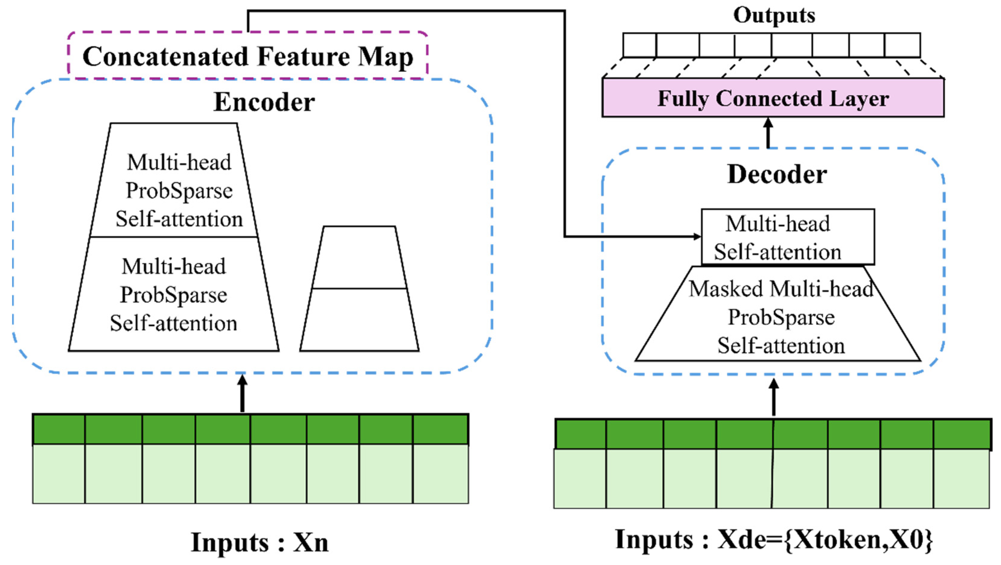
Informer is an improved Transformer model specifically designed for long-term time-series forecasting. While maintaining high prediction accuracy, it achieves efficient computation and better generalization in long-sequence tasks. The overall framework of Informer is similar to that of the Transformer; however, it introduces a sparse self-attention mechanism, hierarchical feature extraction, and a generative decoder to enhance prediction efficiency and accuracy.

The framework of the Informer model is illustrated in the following Figure 1 [24]:

(1)

Sparse Attention Mechanism

Unlike the standard self-attention mechanism, the core idea of sparse attention is to use probabilistic methods to select only the most important attention weights for computation while ignoring those that have minimal impact on the results. Informer introduces the Probsparse Self-Attention mechanism, which employs a probabilistic sampling strategy to select significant Q–K pairs for computation, thereby reducing computational complexity.

In time-series data, only a small portion of query vectors $Q_i$ contribute substantially to the overall attention distribution, while others have relatively uniform distributions and can thus be neglected. To identify these important queries, Informer measures the divergence of each attention distribution using the Kullback–Leibler (KL) divergence. A larger KL divergence value indicates a more significant attention distribution. The sparsity measurement formula for the $i$-th query vector $q_i$ is defined as follows:

$$M\left(q_i,k\right)=\log \left(\sum _{j=1}^L{e}^{{\displaystyle \frac{q_i{k}_j^T}{\sqrt{d_k}}}}\right)-{\displaystyle \frac{1}{L}}\sum _{j=1}^L{\displaystyle \frac{q_i{k}_j^T}{\sqrt{d_k}}}$$

(1)

In this formula, the term $\log \left({\sum }_{j=1}^L{e}^{{\displaystyle \frac{q_i{k}_j^T}{\sqrt{d_k}}}}\right)$ represents the Log-Sum-Exp (LSE) operation, which measures the potential attention intensity generated by the interaction between the query $q_i$ and all keys from an exponential–probability distribution perspective. The term ${\displaystyle \frac{1}{L}}{\sum }_{j=1}^L{\displaystyle \frac{q_i{k}_j^T}{\sqrt{d_k}}}$ denotes the average scaled similarity between the query $q_i$ and all keys ${ k}_j$. The difference between these two terms quantifies the sharpness of the attention distribution of the query vector $q_i$ relative to a uniform distribution. A higher degree of sharpness larger $M$ value indicates that the query $q_i$ is more important, whereas a smaller $M$ value—closer to a uniform distribution—implies that the query contributes less and can even be disregarded.

Further simplifying the above equation yields:

$$\overline{M}\left(q_i,K\right)=\underset{j}{\mathit{max}}\left\{{\displaystyle \frac{q_i{k}_j^T}{\sqrt{d}}}\right\}-{\displaystyle \frac{1}{L_k}}\sum _{j=1}^{L_k}{\displaystyle \frac{q_i{k}_j^T}{\sqrt{d}}}$$

(2)

As shown in the above equation, a set of query vectors $\overline{Q}$ with the highest scores is selected to participate in the attention computation. The calculation formula for the sparse attention mechanism is as follows:

$$Attention\left(Q,K,V\right)=Softmax\left({\displaystyle \frac{\overline{Q}{K}^T}{\sqrt{d_k}}}\right)V$$

(3)

In the formula, $Q$ denotes the query matrix, $K$ the key matrix, $V$ the value matrix, and $d_k$ represents the dimension of the key matrix.

(2)

Hierarchical Feature Extraction

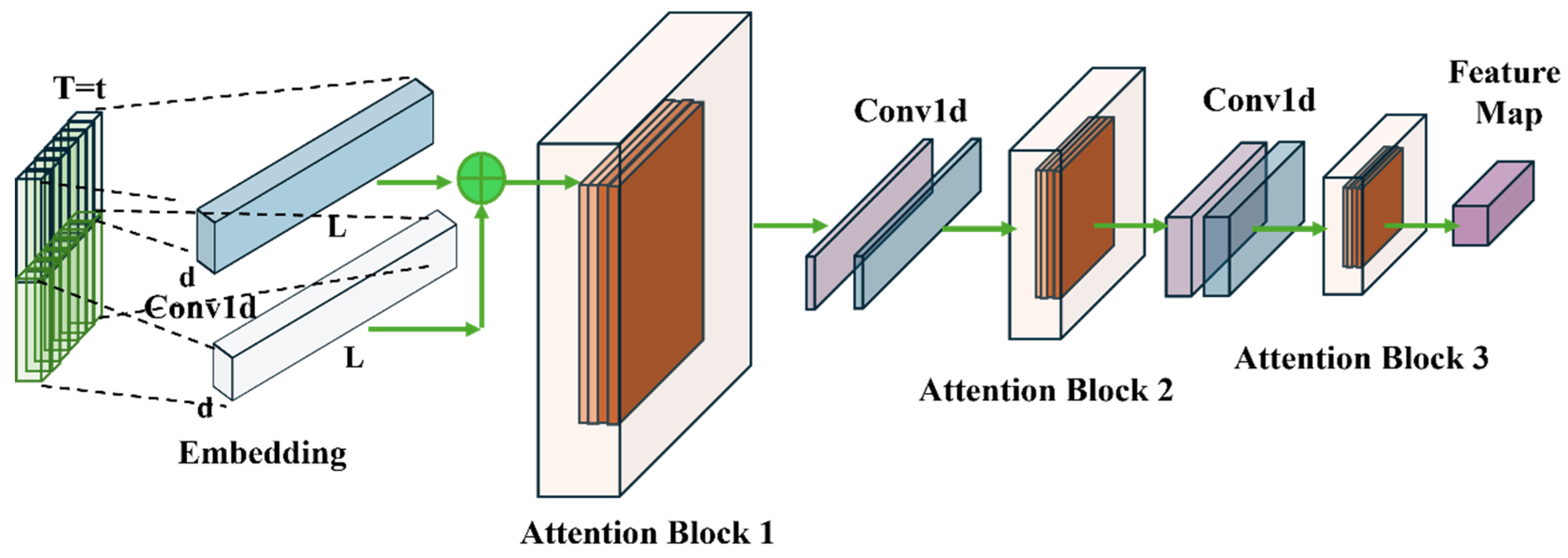
From (1), it can be seen that in the ProbSparse self-attention mechanism, many values are filled using the average of $V$, which can easily lead to severe information redundancy. To address this issue, convolution and pooling operations are applied between adjacent attention modules to perform feature downsampling. Specifically, after each attention layer, an information distillation layer is added to compress the time dimension, extract multi-scale temporal features, remove redundancy, and preserve key trend components.

The workflow of the distillation mechanism is illustrated in the following Figure 2:

As shown in the Figure 2, the steps of the information distillation layer mainly consist of two parts:

(1)

One-dimensional convolution for extracting local multi-scale features

The convolution kernel slides along the time dimension, effectively extracting local patterns within different time windows:

$$Y^{\left(l\right)}=ELU\left(Conv1D\left(LayerNorm\left(X^{\left(l\right)}\right)\right)\right)$$

(4)

where $X^{\left(l\right)}$ represents the input features of the $l$-th layer, $LayerNorm$ denotes layer normalization, $Conv1D$ is the one-dimensional convolution operation, and $ELU$ is the activation function.

By aggregating features from adjacent time steps based on the kernel size, local temporal patterns are captured at various scales. Since different layers use convolution kernels of different sizes, a multi-scale hierarchical structure of temporal features is formed.

(2)

Max-pooling Downsampling

After the convolution operation, a pooling operation is performed. Common pooling methods include average pooling and max pooling. To reduce computational complexity while preserving important feature scales, this study adopts the max-pooling method for downsampling:

$${ X}^{\left(l+1\right)}=Maxpool1D\left(Y^{\left(l\right)},stride=n\right)$$

(5)

In the formula, $stride$ refers to the step size of the convolution kernel along the time dimension, which directly determines the compression ratio of the sequence length. Typically, the stride is set to 2 in the model, allowing the sequence length to be reduced by half, thereby further decreasing computational complexity.

(3)

Generative Decoder

Traditional decoders, such as the Transformer decoder, employ an autoregressive algorithm to generate predictions step by step. However, this approach often leads to error accumulation and limits the model’s ability to capture long-term trends. In contrast, the generative decoder in the Informer model generates the entire future sequence in a single forward pass. By combining multi-layer attention with information from the input sequence, it enables end-to-end multi-step forecasting.

The decoder in Informer mainly consists of two components: One is the real values $X_{token}$ extracted from the tail of the input sequence, and the other is the target values $X_0$ to be predicted. The input sequence of the decoder, $X_{feed\_de}$, is computed as follows:

$$X_{feed\_de}=Concat\left(X_{token}, X_0\right)$$

(6)

2.2. Squeeze-and-Excitation (SE) Module

The SEnet (Squeeze-and-Excitation Network) module explicitly models the inter-channel dependencies and dynamically assigns weights to each feature channel, thereby enhancing the feature representation capability. By effectively integrating the SEnet module with the Informer model, this study leverages Informer’s long-sequence modeling ability together with SEnet’s feature recalibration capability to achieve accurate prediction of temperature-induced strain [25,26].

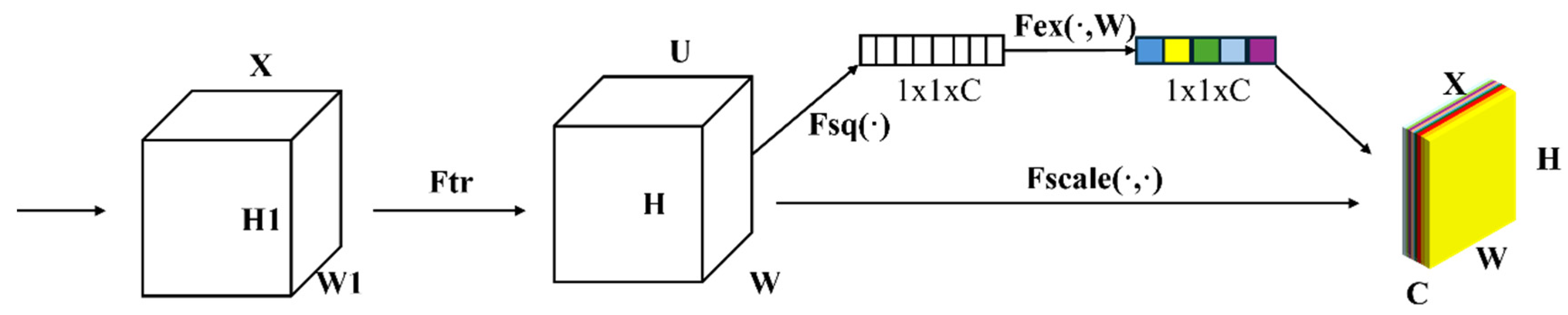
The architecture of the SEnet module is illustrated in the following Figure 3.

As shown in the Figure 3, the SEnet module mainly consists of two parts: Squeeze (global information compression) and Excitation (inter-channel dependency modeling). The underlying principles are as follows:

(1)

Squeeze Module

The purpose of this module is to compress the spatial or temporal dimensional information into a global descriptive vector, enabling the model to focus on global context rather than local features. This is achieved by performing a global average pooling operation on each channel to compress the data information.

The formula for global average pooling is as follows:

$${ z}_c={\displaystyle \frac{1}{H\times W}}\sum _{i=1}^H\sum _{j=1}^W{X}_c\left(i,j\right)$$

(7)

In this formula, $H$ denotes the height of the feature map, $W$ represents its width, $i$ is the index along the height dimension, and $j$ is the index along the width dimension. $X_c\left(i,j\right)$ represents the element at position $\left(i,j\right)$ in the $c$-th channel of the feature map.

(2)

Excitation Module

The purpose of this module is to enable the model to learn the relationships between different channels, allowing it to determine which channels are more important. This is achieved through a two-layer fully connected network, which captures inter-channel dependencies and performs channel-wise feature recalibration. The calculation formula is as follows:

$$s=\sigma \left(W_2\delta \left(W_{1}z\right)\right)$$

(8)

In the formula, $W_1\in {\mathcal{R}}^{{\displaystyle \frac{C}{r}}\times C}$ denotes the compression weight matrix, and $W_2\in {\mathcal{R}}^{C\times {\displaystyle \frac{C}{r}}}$ denotes the expansion weight matrix. The parameter r represents the channel reduction ratio; $\delta \left(·\right)$ refers to the ReLU activation function, and $\sigma \left(·\right)$ represents the Sigmoid activation function. The vector $s\in {\mathcal{R}}^C$ corresponds to the channel-wise attention weights (or sparsity weights) for each channel.

3. Experimental Setup

Based on the architectural introduction of deep learning foundational networks and the subsequent improvements and innovations made upon the Transformer model, a series of experiments and analyses were conducted to further demonstrate the accuracy and reliability of the proposed model in multivariate long-term time-series forecasting. First, the data used in this study were obtained from real bridge structural monitoring datasets and publicly available datasets, collected from different bridge monitoring systems. This diversity ensures the generalizability and robustness of the experimental results. Moreover, three widely used performance metrics—Root Mean Square Error (RMSE), Mean Absolute Error (MAE), and the Coefficient of Determination (R²)—were employed to comprehensively evaluate the model’s performance in time-series prediction tasks. Subsequently, the specific parameter settings of the proposed model are presented, followed by a brief introduction of the baseline models selected for comparison. These baseline models represent the current state-of-the-art methods in the field of time-series forecasting, providing a solid foundation for validating the effectiveness of the proposed Informer-SEnet model.

Through a series of comparative experiments, the superior performance of the Informer-SEnet model in time-series forecasting tasks was verified. Furthermore, to assess the rationality of the model design, a set of ablation experiments was conducted by sequentially removing individual components of the model and analyzing their impacts on overall performance.

3.1. Data Sources

In deep learning research, the performance of models highly depends on both the quality and quantity of data. To ensure the reliability and persuasiveness of the prediction results, this study employs measured data and public datasets as the primary data sources. Both datasets originate from physical data collected by structural health monitoring (SHM) systems installed on real bridges.

(1) Measured Datasets: Two sets of measured data are used in this study, both obtained from different cross-sectional strain monitoring points within the long-term structural health monitoring system of a bridge. The measured dataset 1 originates from data of strain sensor at section 6, while the measured dataset 2 comes from the strain sensor at section 5. 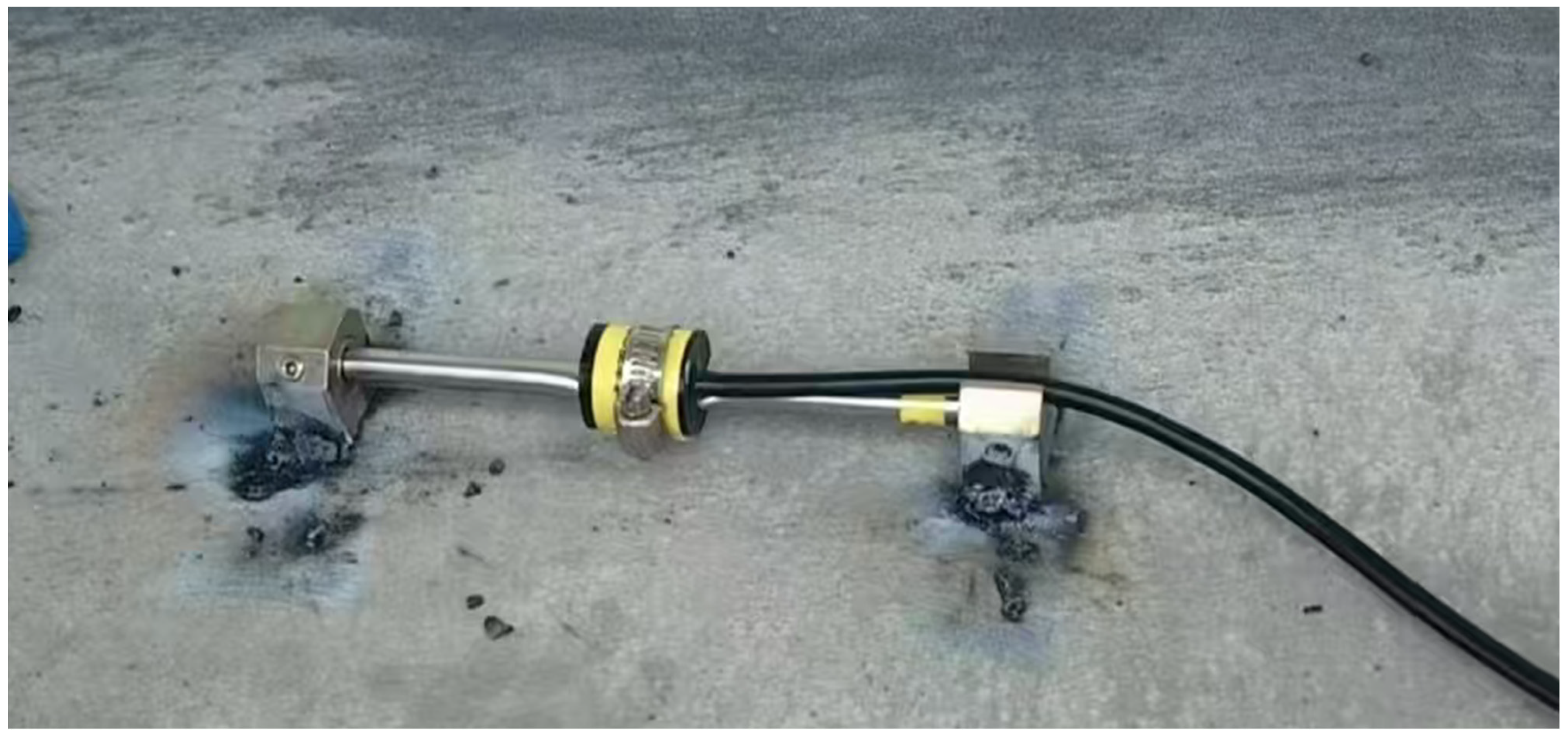The layout diagram of the strain measurement points is shown in Figure 4. The monitoring system is equipped with multiple types of sensors, including strain gauges, temperature sensors, and accelerometers, enabling continuous acquisition of structural responses under varying environmental and loading conditions. The strain sensor used is a vibrating wire strain sensor, as shown in Figure 5. This study focuses primarily on temperature and strain, aiming to investigate the relationship between temperature and temperature-induced strain as a basis for assessing structural safety. In the monitoring system, strain data are collected at a frequency of one sample every 10 min. A total of 4433 data records from November to December 2024 are selected as the dataset. Prior to use, the raw signals underwent outlier removal, missing-data imputation, and temperature-effect separation to ensure the reliability and consistency of the input data.

(2) Public Dataset: The public dataset used in this study originates from a standard open-source resource widely adopted in structural health monitoring research, Bridge-health-monitoring-master. This dataset includes time-series measurements of strain, displacement, temperature, and other structural responses under varying thermal conditions. The deflection sensor records data at a frequency of one sample every 10 min. A total of 4433 data records collected from May to June 2020 are selected as the basis for the present analysis.

3.2. Data Preprocessing

Data quality has a substantial impact on the reliability of experimental results; therefore, ensuring high-quality input data is essential. In this study, an ARIMA-based optimization method is employed to detect and correct abnormal monitoring data. Temperature effects are separated using empirical mode decomposition (EMD), and normalization is applied to enhance prediction accuracy and reduce the risk of model overfitting.

(1)

Handling Anomalous Data

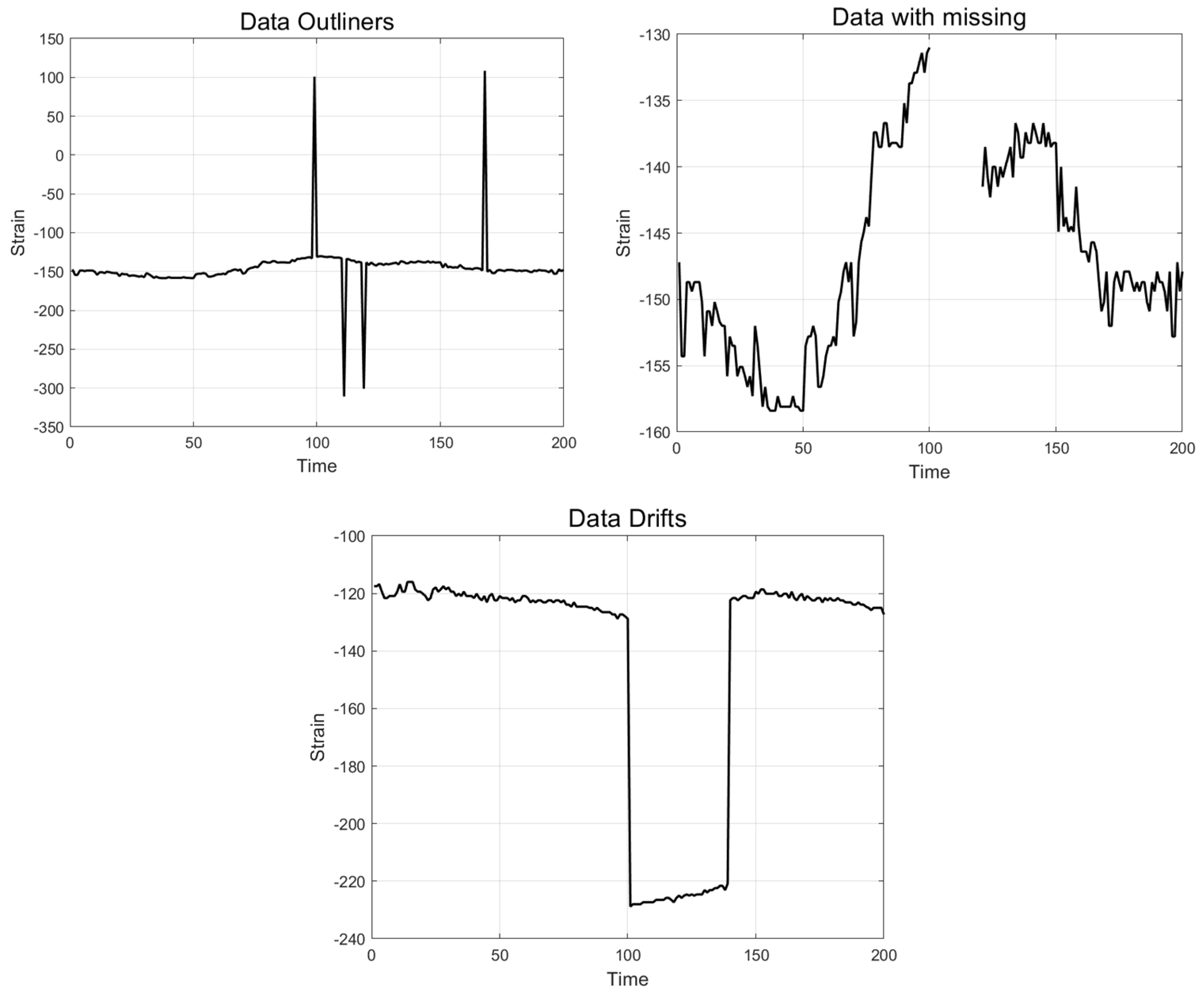
During the long-term data collection process in bridge health monitoring systems, monitoring data may be affected by issues such as equipment malfunctions, data transmission errors, and environmental factors, resulting in data missing, outliners and drift. The common forms of data anomalies are illustrated in Figure 6 below.

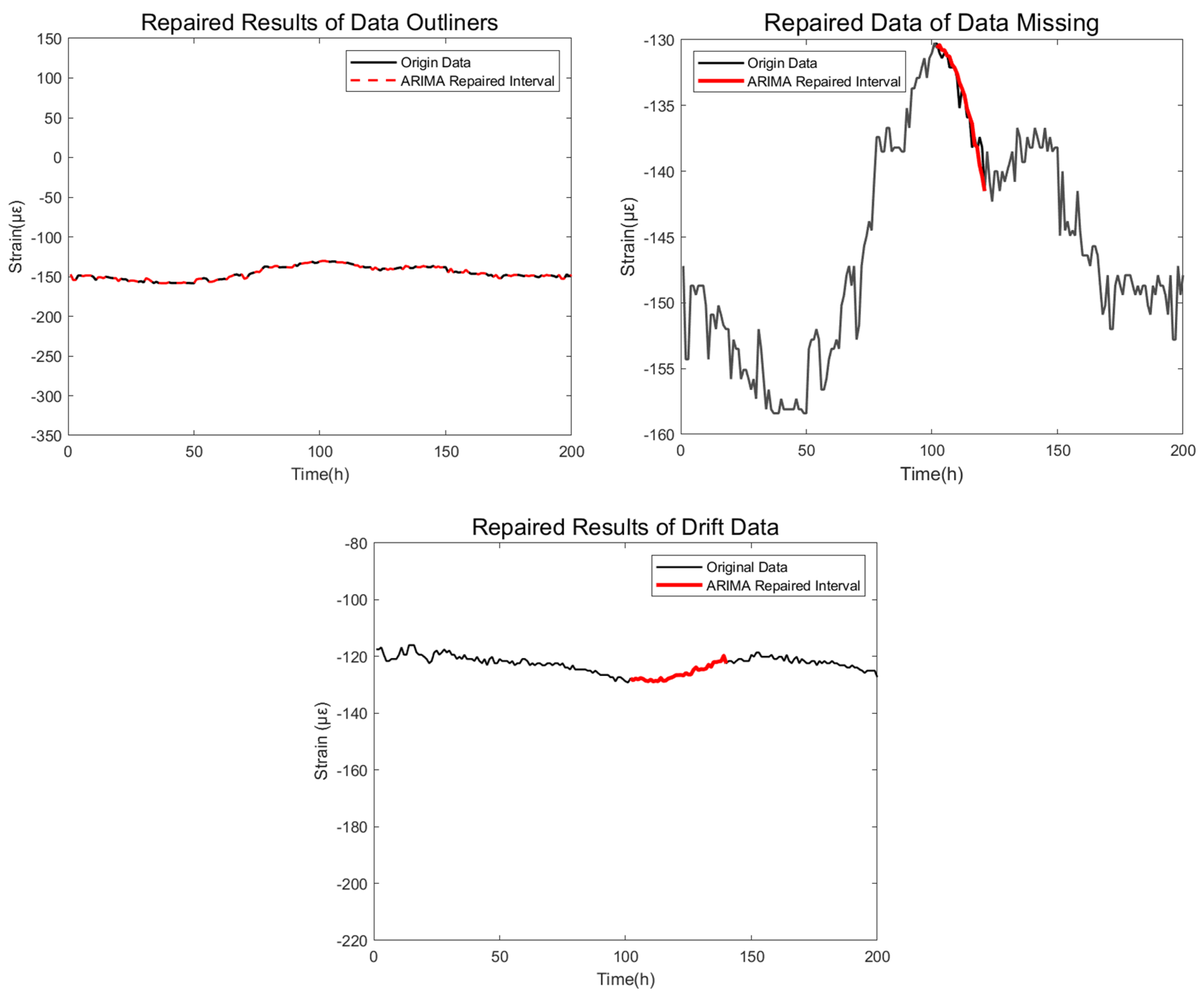
To address data anomalies, this study employs the ARIMA [27] optimization algorithm for anomaly detection and cleaning before conducting experiments. A preliminary data cleaning process is first applied to the raw data, followed by the missing value imputation framework to reasonably complete both the missing data and the cleaned data. ARIMA, which stands for AutoRegressive Integrated Moving Average, is a widely used statistical model for time series data analysis and forecasting. The principle of ARIMA-based data preprocessing involves transforming non-stationary time series data into stationary data through differencing. A model is then established by regressing the dependent variable on its lagged values and the present and lagged values of the random error term. In this study, the ARIMA model is used as a forecasting tool to model time series data. Anomalies are detected by analyzing the model residuals, and the ARIMA-based prediction correction strategy is applied to address different types of anomalous data. This improves the completeness and validity of the data. The data recovery results are shown in Figure 7 below.

(2)

Data Normalization Process

Deep learning models often encounter challenges when dealing with non-standardized data, such as irregular value changes, excessively large data values, and inconsistent data scales, which can affect training speed, convergence efficiency, and overall performance. Data normalization helps accelerate model convergence, prevents gradient vanishing or explosion, improves model performance, and enhances numerical stability. Therefore, in this study, both input and output data are normalized using the Min-Max normalization method, mapping the data to the range of [0, 1]. This approach efficiently handles large datasets while preserving the original relationships between the data. The relevant formulas are as follows:

$$X_t={\displaystyle \frac{X_t-X_{min}}{X_{max}-X_{min}}}$$

(9)

$${ Y}_t={\displaystyle \frac{Y_t-Y_{min}}{Y_{max}-Y_{min}}}$$

(10)

In the formula, $X_t$ and $Y_t$ represent the true values at time $t$; $X_{max}, Y_{max}$ are the maximum values of the input and output data, respectively; $X_{min}$ and $Y_{min}$ are the minimum values of the input and output data.

(3)

Temperature Effect Separation

In bridge health monitoring, strain or deflection data often contain both high-frequency live load effects and low-frequency temperature effects, with the latter being mixed in the data, which can cause interference and affect the scientific accuracy of the evaluation. To enhance the prediction accuracy of structural response in deep learning models, this study employs the Variational Mode Decomposition (VMD) method for temperature effect separation before inputting the data. VMD is an adaptive signal decomposition technique that determines the number of modes based on the actual data and adaptively matches the optimal center frequency and bandwidth for each mode. Compared to Empirical Mode Decomposition (EMD), VMD avoids modal aliasing and endpoint effects and offers a stronger mathematical foundation [28].

VMD can decompose complex signals into several sub-sequences with different frequencies, which are relatively stationary, making it suitable for non-stationary sequences. By using VMD for temperature effect separation, we can effectively extract the structural response data while eliminating the influence of temperature, thus improving the prediction accuracy. The core idea of VMD is to construct and solve a variational problem to achieve effective signal decomposition. The results of the separation are shown in the Figure 8, Figure 9 and Figure 10 below.

3.3. Dataset Construction

This chapter focuses on the multi-step prediction of the bridge’s multivariate structural response ${\widehat{y}}_T\in \mathbb{R}$ at a future time $T$. To achieve this prediction, in addition to the current temperature information at time $T$, historical observation sequences from the past period before time $T$ must also be included in order to capture the cumulative and delayed effects of temperature changes on structural response. To balance between information sufficiency and computational efficiency, this study uses a fixed-length time window for input, avoiding information redundancy and overfitting caused by excessively long historical sequences. Specifically, let the input time window length be $S$, and the time period covered by the window be $\tau =\left\{T-s+1,\dots \dots T\right\},\forall t\in \tau .$ The input feature information for predicting ${\widehat{y}}_T$ is denoted as $X_T=\{X_{T-s+1},\dots ,X_T\}$.

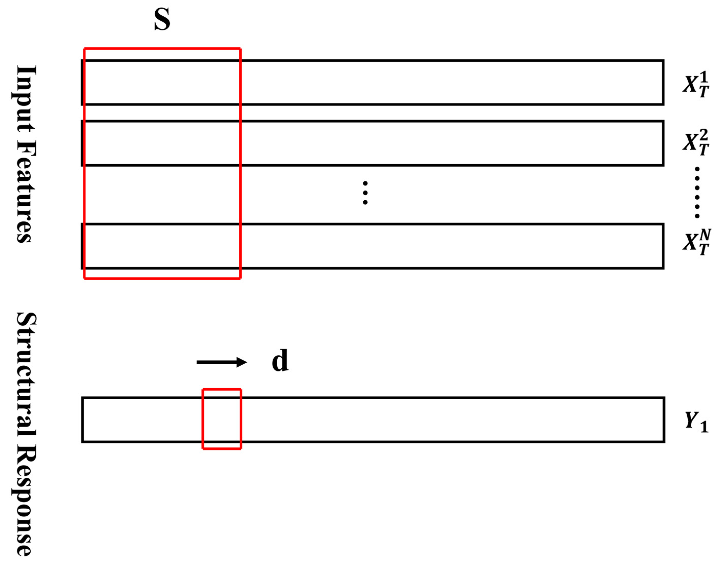
Considering that bridge monitoring data exhibit significant time-series characteristics such as periodicity and trends, to effectively model their dynamic evolution patterns, this study adopts a sliding window approach to construct the dataset. This method uses the observed data from the continuous $S$ historical time steps as the input window and predicts the structural response values for the subsequent $d$ time steps. The data construction method is illustrated in Figure 11 below.

In the specific implementation, the temperature feature sequence and the structural response sequence are simultaneously divided into windows. Let the length of the original sequence be $N$, the window length be $S$, and the sliding step size be $d$. After the division, the input feature matrix $X$ and the corresponding label matrix $Y$ are constructed as follows:

$$X=\left[\begin{array}{ccc}\begin{array}{cc}{x}_1& x_2\\ x_2& x_3\end{array}& \dots & \begin{array}{cc}{x}_{s-1}& x_s\\ x_s& x_{s+1}\end{array}\\ ⋮& \ddots & ⋮\\ \begin{array}{cc}{x}_{N-s}& x_{N-s+1}\\ x_{N-s+1}& x_{N-s+2}\end{array}& \dots & \begin{array}{cc}{x}_{N-2}& x_{N-1}\\ x_{N-1}& x_N\end{array}\end{array}\right],Y=\left[\begin{array}{c}\begin{array}{c}{y}_s\\ y_{s+1}\end{array}\\ ⋮\\ \begin{array}{c}{y}_{N-1}\\ y_N\end{array}\end{array}\right]$$

(11)

where the input of the $t$-th sample is $X_t=[x_t,x_{t+1},\dots ,x_{t+s-1}{]}^T$, and the corresponding label is $Y_t=[y_{t+s},y_{t+s+1},\dots ,y_{t+s+d-1}{]}^T$. That is, the model uses the continuous $S$ observation values starting from time $t$ to predict the structural response for the next $d$ time steps.

In this experiment, based on the data time resolution and the physical characteristics of bridge response changes, after multiple experiments and validation, the window length is set to S = 143 (one day), and the prediction step size d = 143 (the next day), in order to balance capturing long-term trends and short-term fluctuations. After this division, a total of N − S + 1 valid samples are obtained. Finally, all samples are randomly divided into training, validation, and test sets in a 7:2:1 ratio, ensuring that there is no overlap in time across the sets, allowing for an objective evaluation of the model’s generalization ability.

3.4. Evaluation Metrics

To evaluate the prediction performance of the Informer-SEnet model, three commonly used metrics were employed: Root Mean Square Error (RMSE), Mean Absolute Error (MAE), and the Coefficient of Determination (R²). RMSE measures the average magnitude of the difference between the predicted and actual values, providing an intuitive reflection of the model’s prediction accuracy. MAE represents the average of the absolute differences between the actual and predicted values. R² measures the correlation between the predicted and actual values, indicating how well the model fits the data and how closely the predicted results match the true observations. A smaller RMSE and MAE and a larger R² indicate better prediction performance and higher model accuracy. The formulas for these evaluation metrics are as follows:

$$\mathrm{R}\mathrm{M}\mathrm{S}\mathrm{E}=\sqrt{{\displaystyle \frac{1}{n}}\sum _{i=1}^n{\left({\widehat{y}}_i-y_i\right)}^2}$$

(12)

$$\mathrm{M}\mathrm{A}\mathrm{E}={\displaystyle \frac{1}{n}}\sum _{i=1}^n\left|y_i-{\widehat{y}}_i\right|$$

(13)

$${\mathrm{R}}^2=1-{\displaystyle \frac{{\sum }_{i=1}^n{\left(y_i-{\widehat{y}}_i\right)}^2}{{\sum }_n^{i=1}{\left(y_i-\overline{y}\right)}^2}}$$

(14)

In the above formulas: $n$ represents the number of samples, $y_i$ denotes the actual (true) value, ${\widehat{y}}_i$ denotes the predicted value, and $\overline{y}$ represents the mean of the actual values.

3.5. Parameter Settings

The experimental methods in this chapter are implemented in a Python 3.9 development environment using the Pytorch deep learning framework, with the experiments running on a Windows 11 operating system. The hyperparameters used in the experiments are based on the parameter settings commonly found in similar deep learning models.

The Informer architecture consists of encoder and decoder layers. To prevent overfitting caused by excessive layers and to improve the generalization ability of the model, this study sets the decoder layers to 2 and the encoder layers to 3. Each encoder and decoder layer includes multi-head attention mechanisms, feedforward layers, and hidden layers. Since the self-attention mechanism in Informer relies heavily on a large feature space to learn global dependencies, a high number of hidden layers increases the computational load, while too few hidden layers may reduce feature fitting ability. Through multiple experiments, the hidden layer size was set to 256 to balance computational cost and model expressive power. The multi-head attention mechanism allows the model to capture different feature patterns in the sequence from various subspaces, and setting the number of heads to 8 effectively enhances the attention mechanism’s expressive power while avoiding excessive computational burden. The feedforward neural network enhances the model’s ability to fit non-linear relationships and allows the model to extract higher-order features from the attention outputs. The dimension of the feedforward network is typically set to 8 times the size of the hidden layer.

To prevent overfitting, a Dropout regularization layer is added after the fully connected layers in both the encoder and decoder layers, with a dropout rate of 0.1. This mechanism randomly masks 10% of the neurons, preserving important features. The batch size refers to the amount of data input into the network during each iteration. A smaller batch size results in longer training times and slower convergence, and can cause large gradient fluctuations, making training unstable. Increasing the batch size can speed up training but may degrade the model’s generalization ability. After considering both computational speed and model performance, a batch size of 64 was chosen. The ReLU activation function is used, which offers high computational efficiency, alleviates gradient vanishing, accelerates convergence, produces sparse activations, and enhances the model’s generalization ability. The number of training iterations is crucial; too few iterations may lead to underfitting, while too many may cause overfitting. In this study, after observing the loss curves for the training and validation sets, and considering the model’s complexity and learning rate, the final training iterations were set to 120. The parameter settings for the Informer model are shown in

Table 1. Hyperparameter Settings for the Informer Module.

Parameter Name	Parameter Value	Parameter Name	Parameter Value	Parameter Name	Parameter Value
Hidden Features	256	Number of Decoder Layers	2	Batches	64
Multi-Head Attention Mechanism	8	Feed-Forward Layer Dimension	2048	Number of Training Iterations	120
Number of Encoder Layers	3	Activation Function	ReLu	Dropout	0.1
Learning Rate	0.0001	Loss Function	MSE	Time Step Size	24

below:

The SE (Squeeze-and-Excitation) module consists of two main components: First, the Squeeze operation, which uses convolutional pooling to extract global features; second, the establishment of inter-channel dependencies, achieved by a two-layer fully connected network that recalibrates the weights of each channel. A channel size of 64 is commonly used in deep learning as a medium-scale feature channel, providing a good balance of expressiveness and computational efficiency. If the number of channels is too small, the SE module may struggle to learn rich attention weights, while too large a number significantly increases the computational burden. Global average pooling reflects the overall activation strength of each channel and is more stable than max pooling, being less influenced by local anomalies. Therefore, average pooling is selected for convolutional layer pooling computation in this study. The channel compression ratio in the SE module helps to capture the most critical feature information dependencies and improves computational efficiency. In this study, a compression ratio of 16% is chosen to balance the number of parameters, computational efficiency, and model performance. The relevant parameter settings are shown in

Table 2. Hyperparameter Settings for the SEnet Module.

Parameter Name	Parameter Value	Parameter Name	Parameter Value
Number of Channels	64	Activation Function	ReLu, Sigmoid
Channel Reduction Ratio	16%	Pooling Type	Average Pooling

below:

4. Experimental Results and Analysis

In the time-series prediction experiments conducted in this study, to evaluate the generalization performance of the proposed model across different datasets, one public dataset and two real-world bridge monitoring datasets were selected as data sources. Based on the parameter settings of the various modules described previously, both horizontal (cross-model) and vertical (within-model) comparison experiments were designed. Each experimental group was evaluated using multiple statistical performance metrics, including MSE, RMSE, and R², to comprehensively assess the model’s prediction accuracy and reliability from multiple perspectives and dimensions.

4.1. Comparative Experiments

To systematically evaluate the prediction performance of the proposed model, a series of state-of-the-art models in the field of time-series forecasting were selected as baseline models for comparison. These include LSTM, BiLSTM, Transformer, Transformer-Encoder, Informer, and Informer-Encoder, covering both recurrent neural network architectures (RNNs) and their variants, as well as the increasingly popular Transformer-based models and their derivatives.

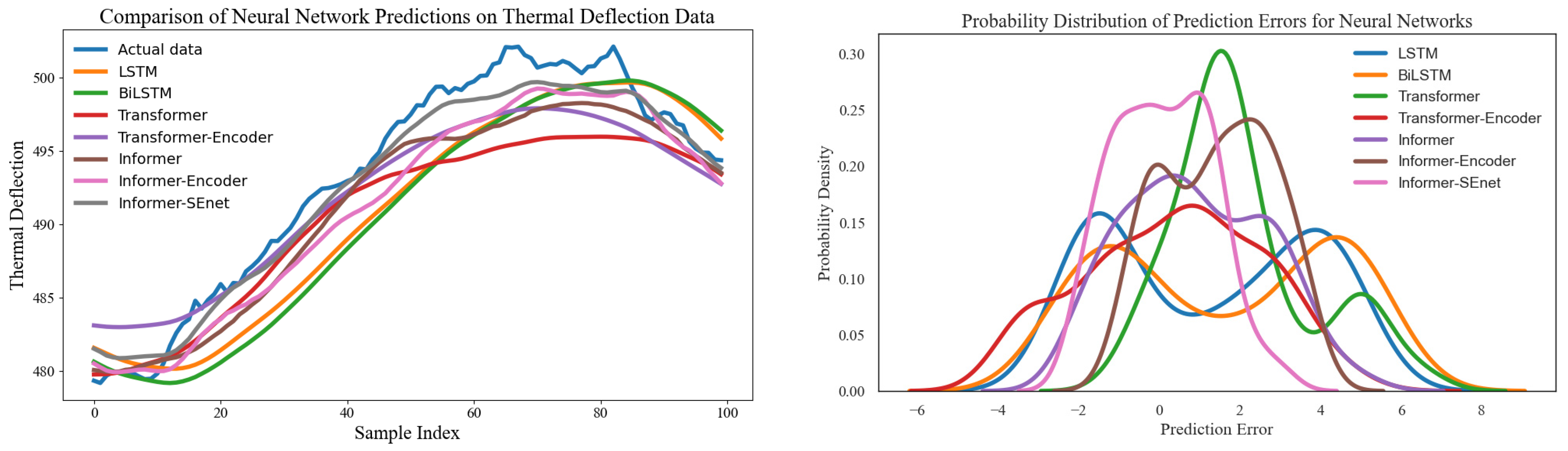
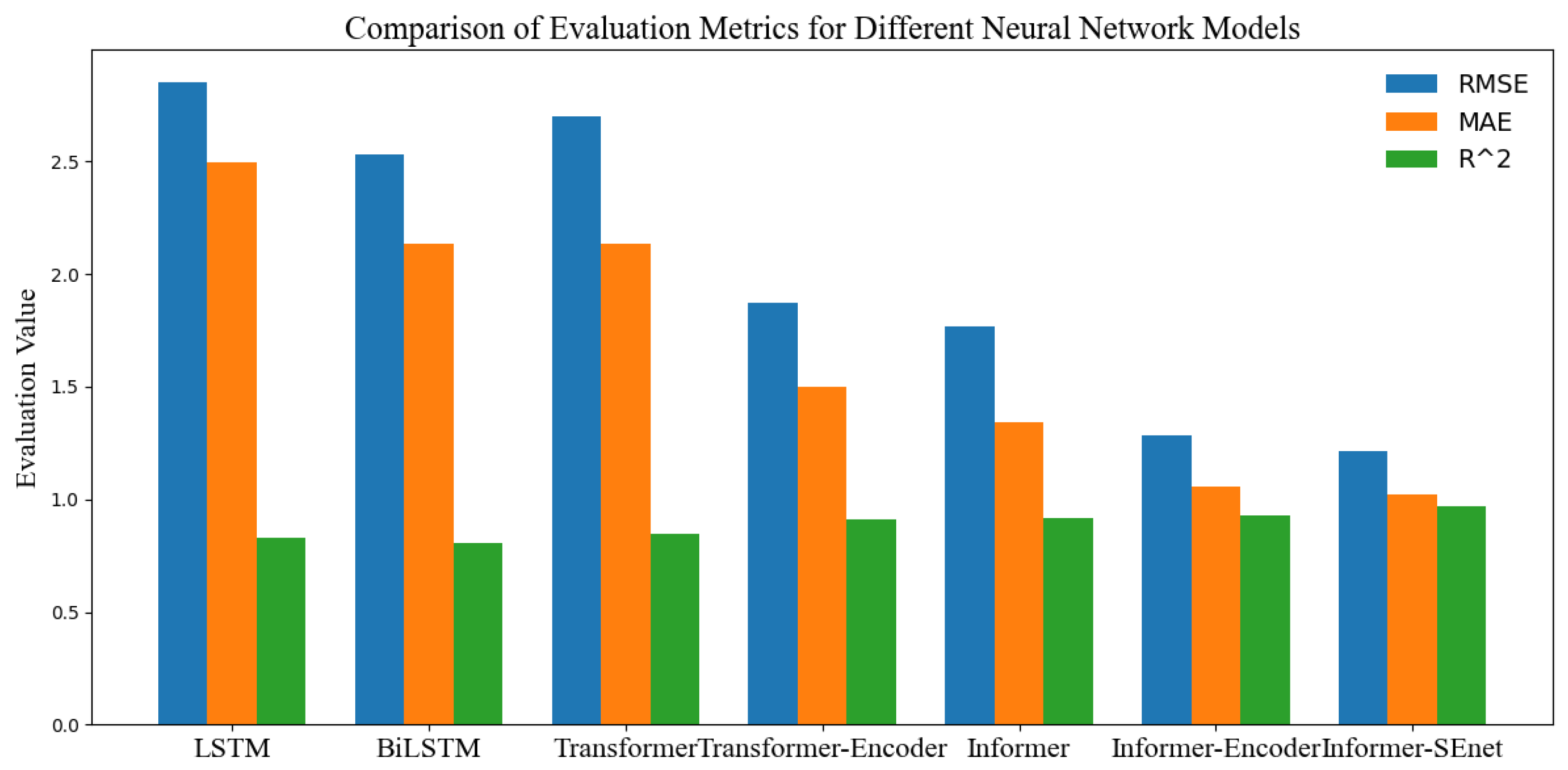
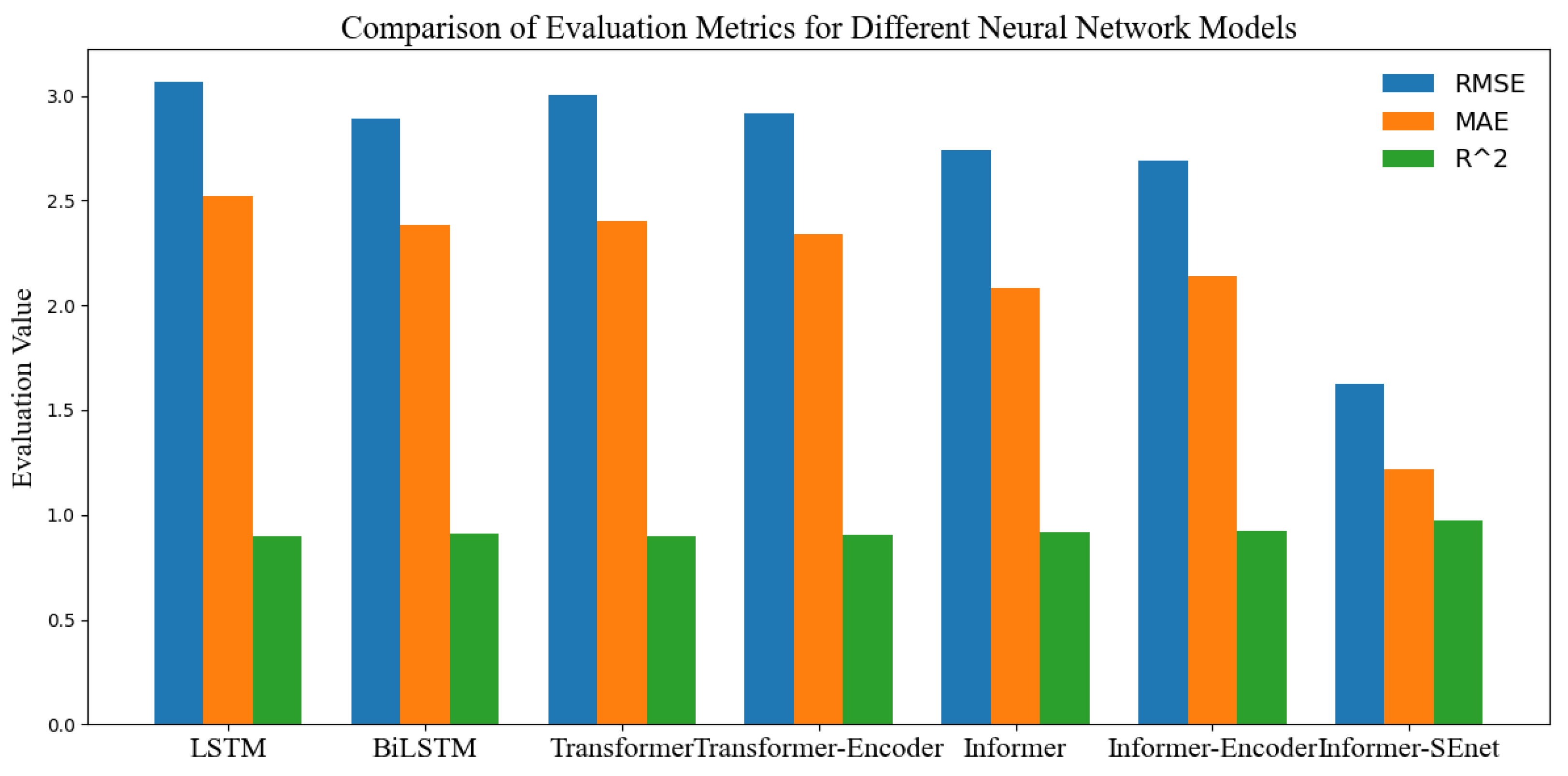
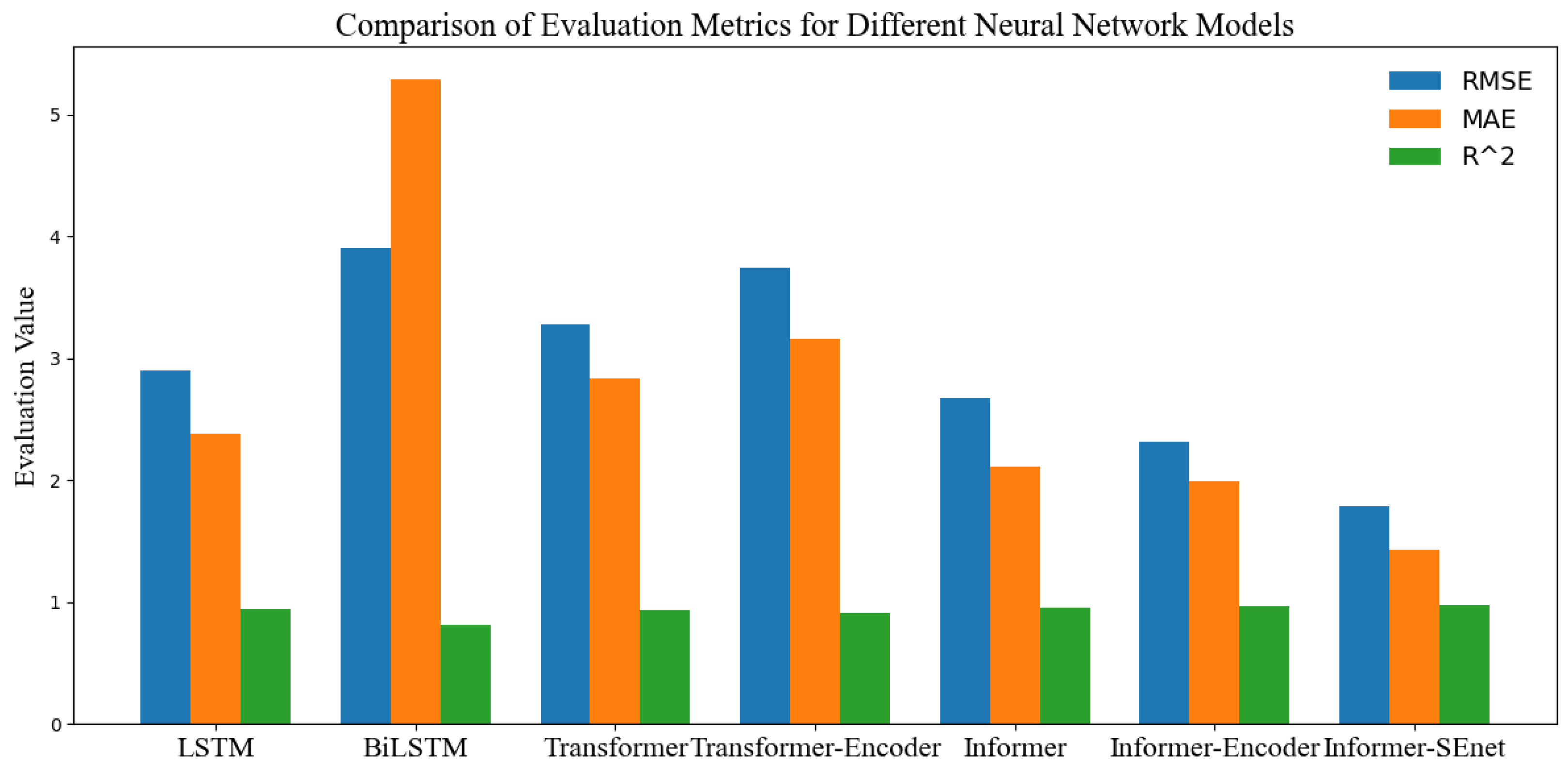
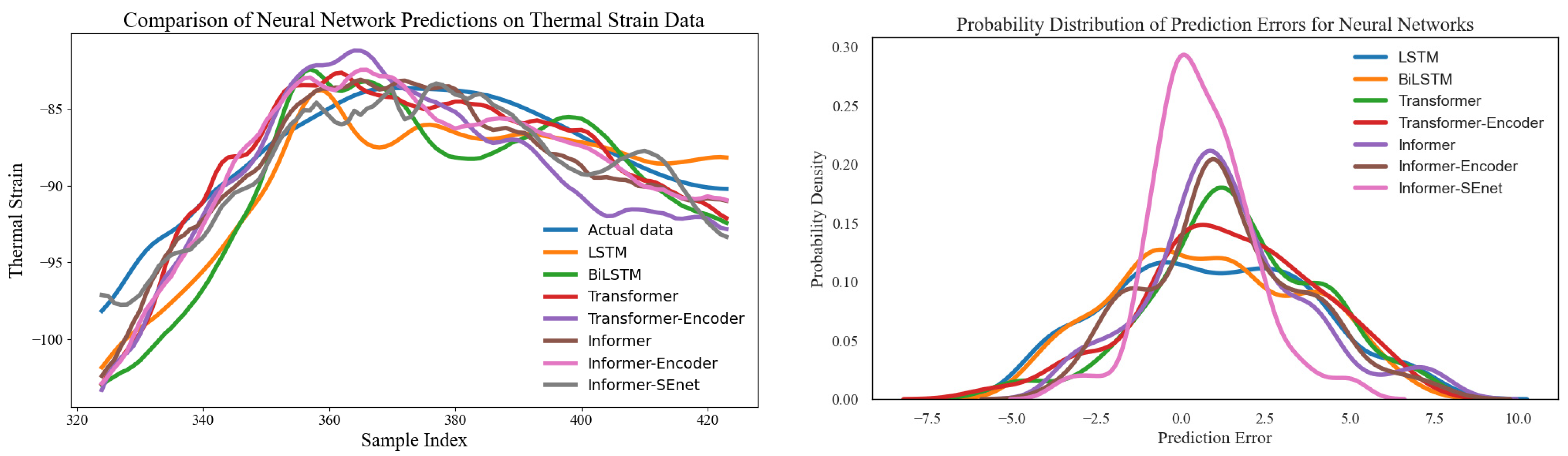
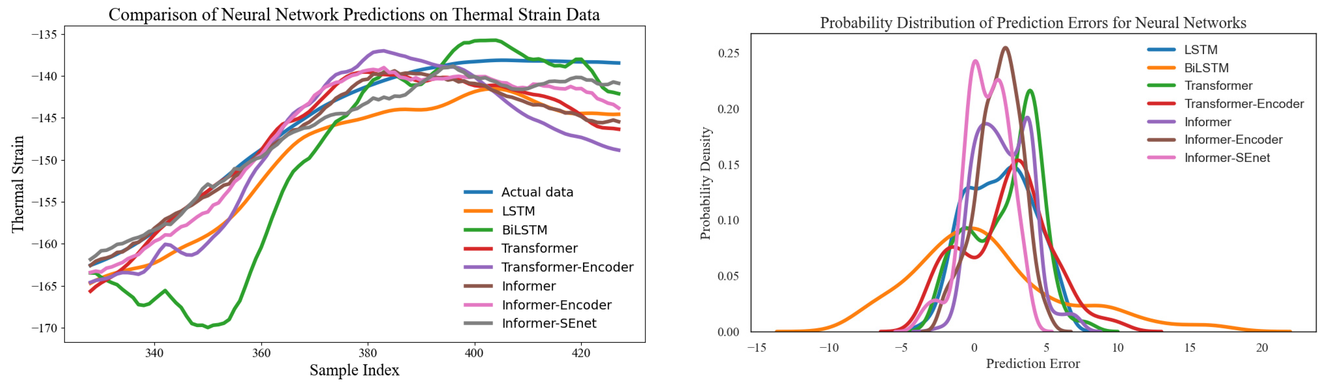
In the comparative experiments, both the public dataset and the measured bridge datasets were used as the data foundation. Based on the periodic variation characteristics of the data, the experimental setup involved using the previous 24 h of data to predict the data trends for the next 24 h. This configuration allows for assessing the accuracy of different models in long-term sequence prediction and evaluating their reliability in capturing long-term temporal dependencies. The experimental comparison results are presented in the following Figure 12, Figure 13, Figure 14, Figure 15, Figure 16 and Figure 17 and

Table 3. Comparative Experimental Results of the Informer-SEnet Model.

Model	Measured Dataset 1			Measured Dataset 2			Open Dataset
	MAE	RMSE	R2	MAE	RMSE	R2	MAE	RMSE	R2
LSTM	2.521	3.068	0.897	2.379	2.904	0.946	2.495	2.854	0.829
BiLSTM	2.386	2.894	0.908	5.293	3.903	0.819	2.137	2.532	0.805
Transformer	2.401	3.002	0.901	2.834	3.283	0.930	2.133	2.699	0.847
Transformer-Encoder	2.338	2.918	0.906	3.165	3.749	0.909	1.498	1.876	0.909
Informer	2.084	2.741	0.917	2.109	2.673	0.953	1.342	1.770	0.915
Informer-Encoder	2.137	2.689	0.921	1.997	2.316	0.965	1.055	1.285	0.926
Informer-SEnet	1.221	1.625	0.971	1.43	1.785	0.979	1.023	1.213	0.969

.

The prediction results of the six comparison models show significant differences in performance across different datasets. The comparison models include traditional LSTM, BiLSTM, and Transformer models and their variants, which have been widely used in time series forecasting in recent years. Traditional recurrent neural networks (such as LSTM and BiLSTM), relying on sequential recursive structures, are prone to issues like gradient vanishing and insufficient long-range dependency capturing, which limits their performance in long-term forecasting tasks like the one in this study. In contrast, Transformer and its variants, using self-attention mechanisms, are better at modeling long-range dependencies, performing overall better than traditional RNN models. However, these baseline models still face issues such as unstable attention distribution, high sensitivity to noise, and insufficient global information compression, resulting in suboptimal performance in engineering data characterized by strong non-stationarity and significant multivariate coupling.

Compared to these baseline models, the proposed Informer-SEnet model integrates sparse self-attention mechanisms and channel attention modules, significantly improving the model’s ability in multi-scale dependency learning, key feature extraction, and noise suppression. In the measured dataset 1, the model outperformed the four comparison models (Transformer, Transformer-Encoder, Informer, Informer-Encoder) with reductions in MAE by 49.16%, 47.78%, 17.05%, and 17.32%, reductions in RMSE by 45.85%, 44.29%, 14.52%, and 15.87%, and increases in R² by 7.73%, 7.07%, 1.13%, and 1.27%, respectively. In the measured dataset 2, MAE was reduced by 49.39%, 54.67%, 31.99%, and 50.61%, RMSE was reduced by 45.63%, 52.39%, 33.21%, and 48.36%, and R² increased by 5.21%, 7.67%, 2.75%, and 6.30%, respectively. On the public dataset, our model also achieved improvements in MAE, RMSE, and R².

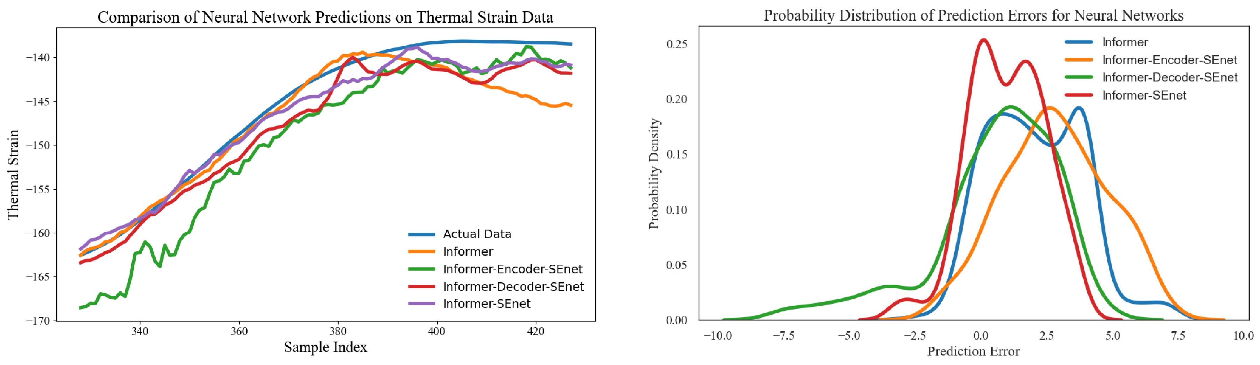
Further analysis of the error distribution shows that all models’ errors approximately follow a normal distribution, but baseline models generally exhibit a “multi-modal” error structure, with larger local errors occurring at trend change points or high-frequency segments. This indicates that the baseline models struggle to capture multi-scale dependencies, sudden changes, and variable coupling relationships. On the other hand, the error distribution of Informer-SEnet is noticeably narrower, with errors mainly concentrated around 0, indicating that the model not only improves overall prediction accuracy but also effectively enhances prediction stability and noise resistance. This phenomenon can be attributed to the following factors: (1) The SE channel attention module strengthens the correlation expression between key variables and suppresses irrelevant or noisy channels. (2) The sparse self-attention mechanism improves the model’s ability to capture global dependencies, preventing excessive distribution of attention over long sequences. (3) The convolutional pooling structure provides local smoothing and feature compression capabilities, making the model more suitable for handling sudden changes and non-stationary characteristics in engineering strain sequences.

In conclusion, whether on measured datasets or public datasets, Informer-SEnet exhibits higher accuracy, stronger stability, and better generalization ability in long-term sequence prediction tasks. Compared to baseline models, the performance advantage of Informer-SEnet is not only reflected in the improvement of metrics but also in its enhanced ability to capture complex non-stationary time series features, fully validating the effectiveness and robustness of the proposed method in multi-variable long-term sequence forecasting.

4.2. Ablation Experiments

To gain a deeper understanding of the contribution and role of each module within the Informer-SEnet model, the model was decomposed into three primary components—Encoder, Decoder, and SEnet—and a series of ablation experiments were conducted. By selectively removing certain components of the model, the study investigated the impact of each module on the overall prediction performance.

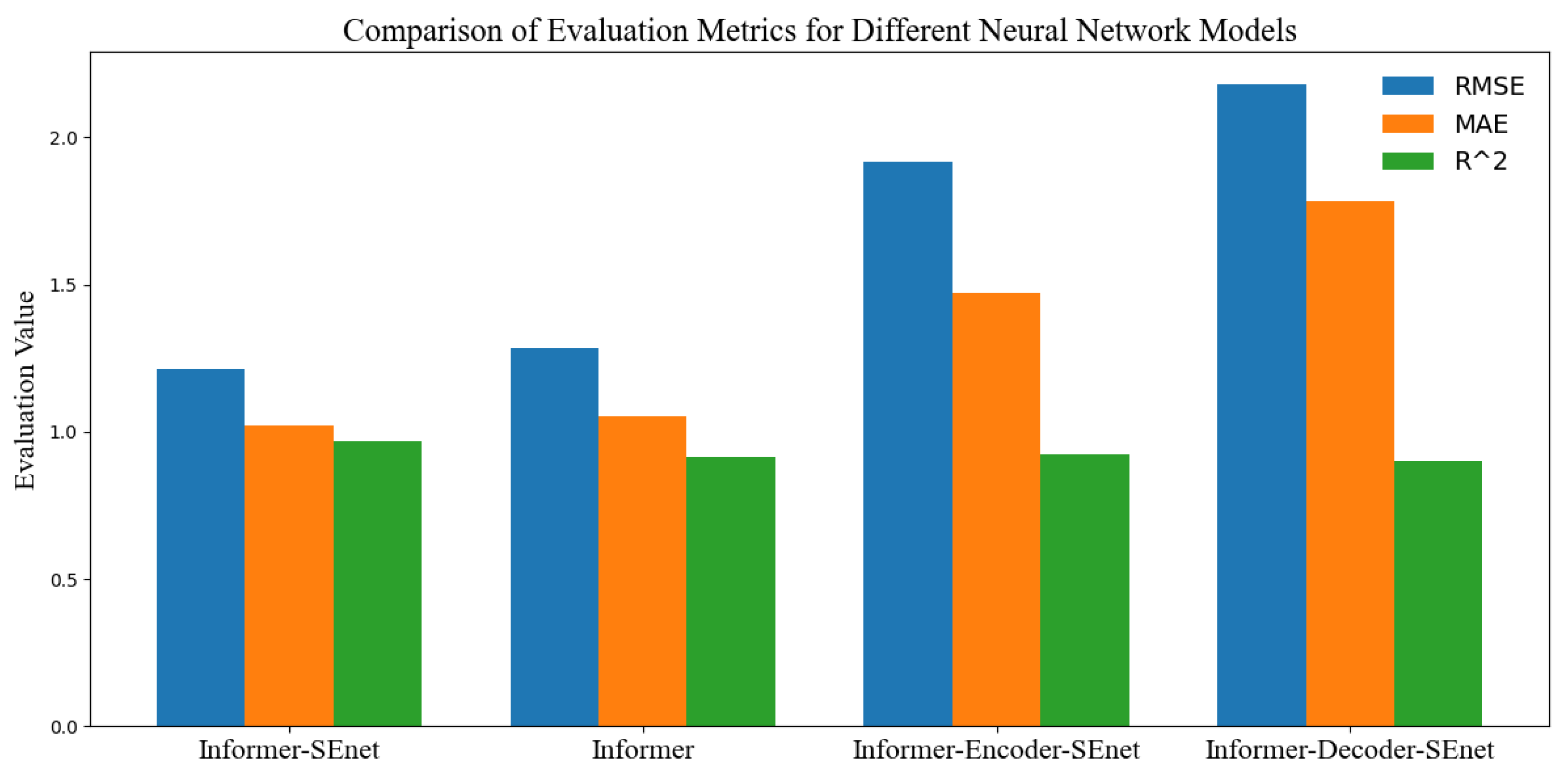
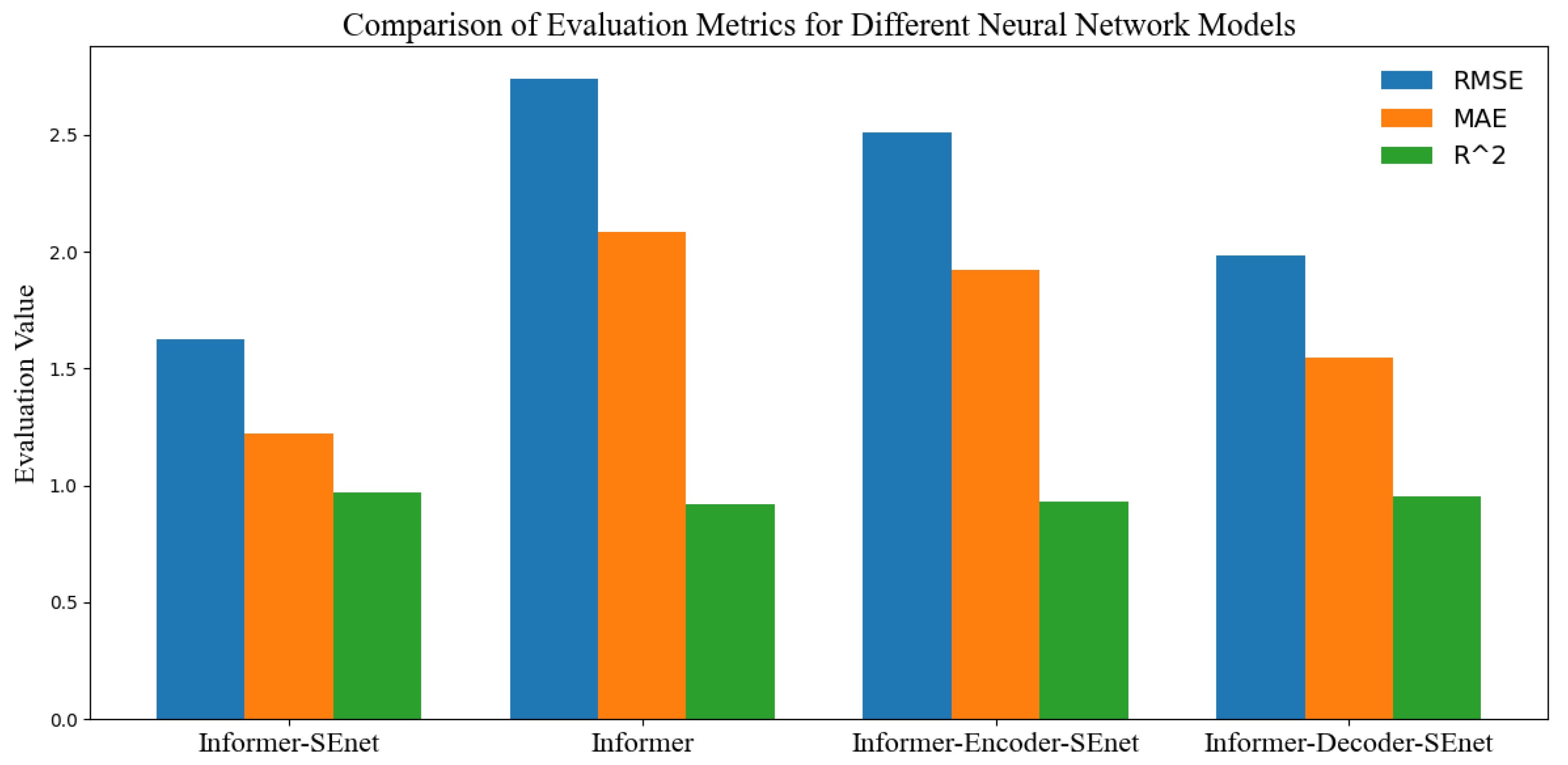
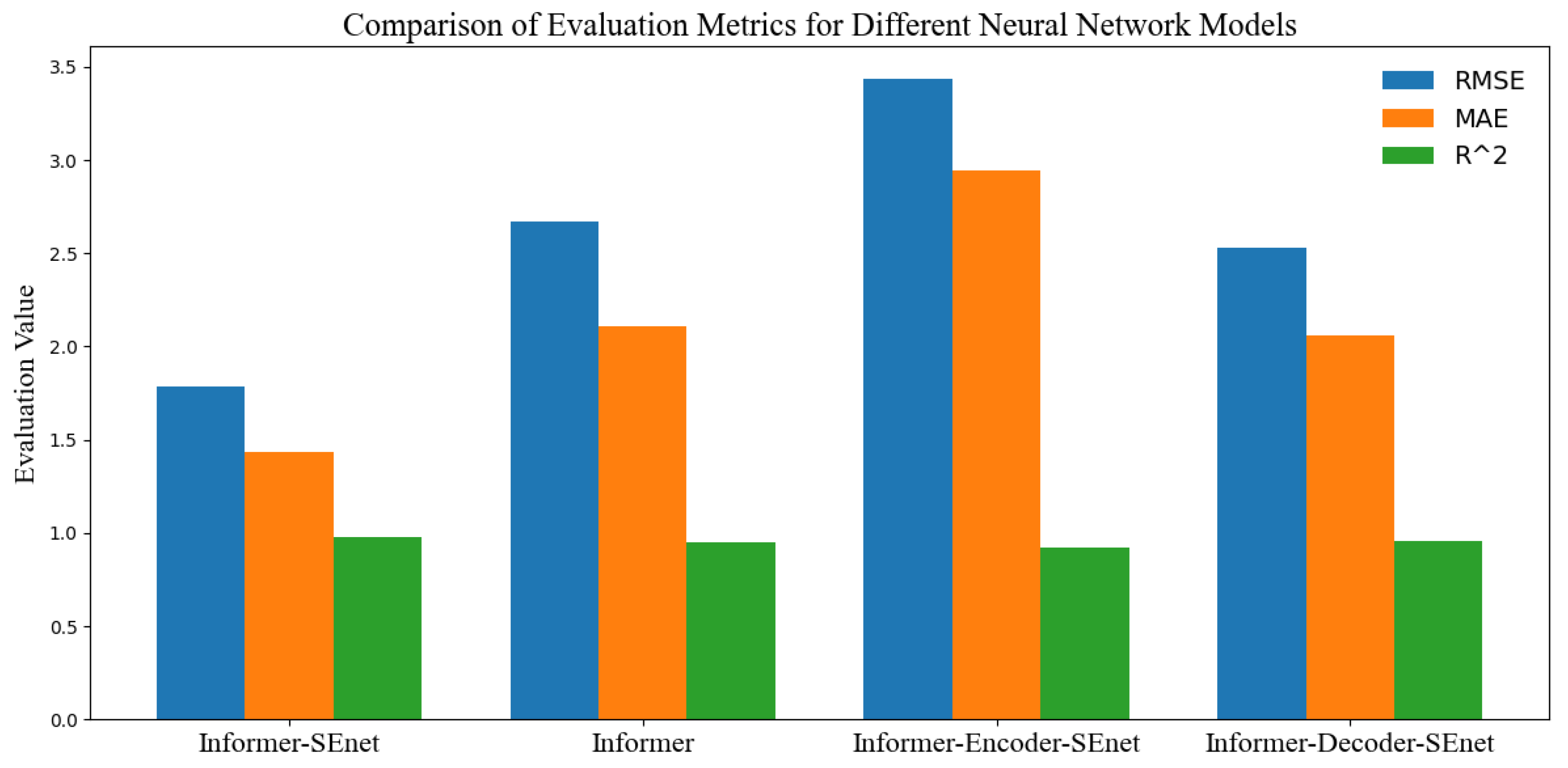
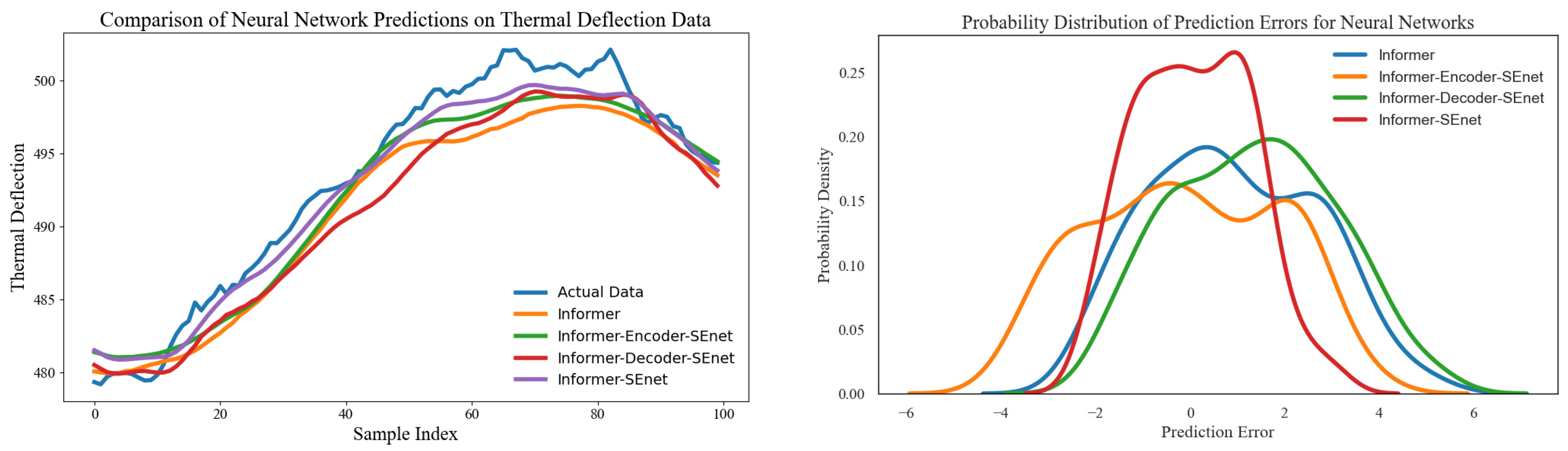
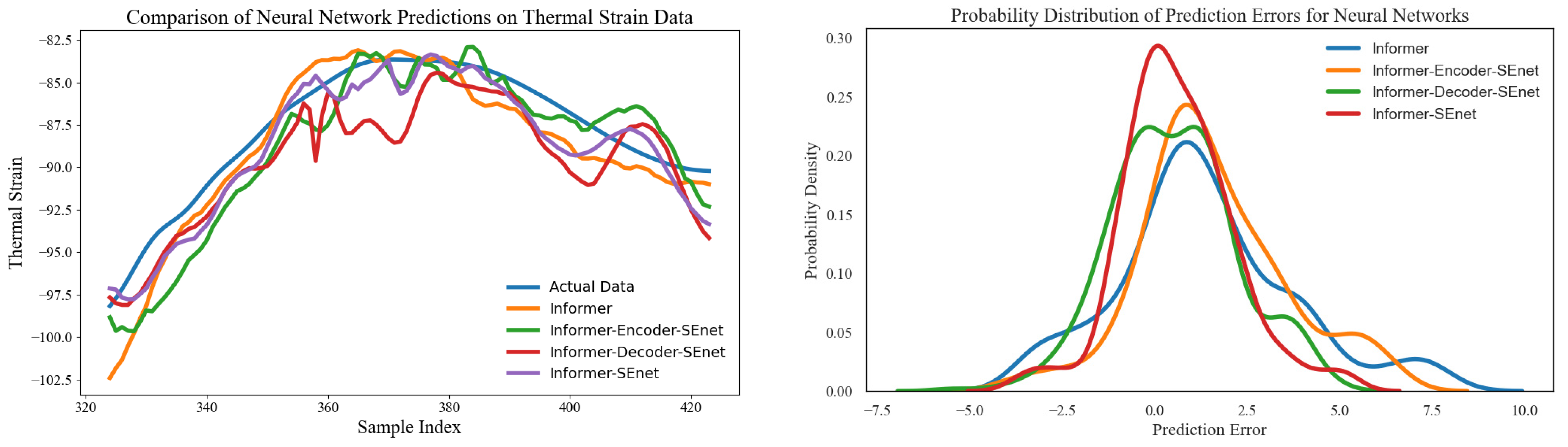
Specifically, three datasets were used to carry out the ablation experiments. The results demonstrate the importance of each component in enhancing the model’s predictive capability. The evaluation metrics used include RMSE, MAE, and R², which provide a comprehensive assessment of model performance. The detailed results of the ablation experiments are presented in the following Figure 18, Figure 19, Figure 20, Figure 21, Figure 22 and Figure 23 and

Table 4. Ablation Experiment Results of the Informer-SEnet Model.

Model	Encoder	Decoder	SEnet	Measured Dataset 1			Measured Dataset 2			Open Dataset
				MAE	RMSE	R2	MAE	RMSE	R2	MAE	RMSE	R2
Basic Model	√	√	√	1.221	1.625	0.971	1.435	1.785	0.979	1.023	1.213	0.969
Variant 1	√	√		2.084	2.741	0.917	2.109	2.673	0.953	1.055	1.285	0.915
Variant 2	√		√	1.921	2.510	0.929	2.944	3.437	0.922	1.474	1.918	0.925
Variant 3		√	√	1.548	1.982	0.956	2.056	2.527	0.958	1.784	2.181	0.900

.

A comprehensive analysis through tables, prediction curves, and error distribution visualizations shows that the proposed Informer-SEnet model performs the best in predicting the future trend of temperature-induced strain, with the smallest errors and the highest stability in fitting. The performance of Variant 1, Variant 3, and Variant 2 decreases sequentially. The differences in performance across models are not only reflected in the changes in metric values but are also closely related to their structural design and the ability to model time-series features.

Firstly, compared to the original Informer, Informer-SEnet introduces a channel attention mechanism and uses the SEnet module to re-weight multivariate time-series features. This allows the model to highlight key features and suppress redundant information. This mechanism effectively enhances the model’s ability to express features in long time series, making it more robust in multi-scale dependency modeling compared to the original Informer. This structural improvement is particularly suitable for handling nonlinear coupling, weak periodicity, and noise interference in temperature-induced strain sequences, which is why its prediction performance is significantly better than the original Informer across all datasets.

Secondly, compared to Informer-SEnet, the predictive performance of the variant model Informer-Decoder-SEnet is slightly weaker, because the removal of the Encoder module weakens two key mechanisms: (1) The absence of the sparse self-attention mechanism makes it difficult for the model to capture long-range dependencies and important contextual relationships; (2) The lack of convolutional pooling reduces the model’s ability to extract local sharp features and smooth background trends.

Therefore, this model shows a significant increase in error at trend turning points, demonstrating that the Encoder plays an irreplaceable role in long-sequence modeling. Similarly, the performance of Informer-Encoder-SEnet further deteriorates, primarily because the Decoder module is removed. The Decoder is a crucial information fusion module in the prediction phase, responsible for mapping the encoded representation to the future prediction space. Without the Decoder, the model can only generate predictions based on the final hidden state of the Encoder, which reduces the capacity to express the prediction space and fails to fully utilize the high-dimensional dynamic features of time series, resulting in significant performance degradation.

In terms of error distribution, all models show errors that approximately follow a normal distribution. However, the baseline variant models generally exhibit a “multi-modal” error characteristic, with large errors occurring at local rapid change segments or trend turning points. This indicates that these models have limited ability to handle non-stationary changes and identify turning points. In contrast, the error distribution of Informer-SEnet is more concentrated, with a narrower range that is primarily focused around zero. This indicates that the model not only achieves higher overall prediction accuracy but also has lower sensitivity to noise, significantly enhancing prediction stability.

4.3. Five-Fold Cross-Validation Experiment

Cross-validation is a powerful model evaluation technique aimed at accurately assessing the model’s generalization ability and avoiding the incidental effects caused by random data splits, further demonstrating the robustness and reliability of the model results. By performing multiple splits and evaluations, cross-validation provides a more stable reflection of the model’s actual performance. Set the dataset as:

$$D=\left\{\left(x_1,y_1\right),\left(x_2,y_2\right),\dots \dots \left(x_n,y_n\right)\right\}$$

(15)

In the equation, $D$ represents the dataset, and $x_n,y_n$ represent the input and output data, respectively.

The basic steps of cross-validation are as follows:

(1)

Divide the dataset $D$ into several non-overlapping subsets: $D_1,D_2,\dots ,D_k$.

(2)

Select one subset as the validation set and the remaining $k-1$ subsets as the training set.

(3)

Train and test the model for each partition, recording performance metrics (such as ${\mathrm{R}}^2$, RMSE, MAE, etc.).

(4)

Take the average of the evaluation results from all rounds as the overall performance estimate of the model:

$$E={\displaystyle \frac{1}{k}}\sum _{i=1}^k{E}_i$$

(16)

In this context, $E_i$ represents the error or performance metric for the $i$-th validation.

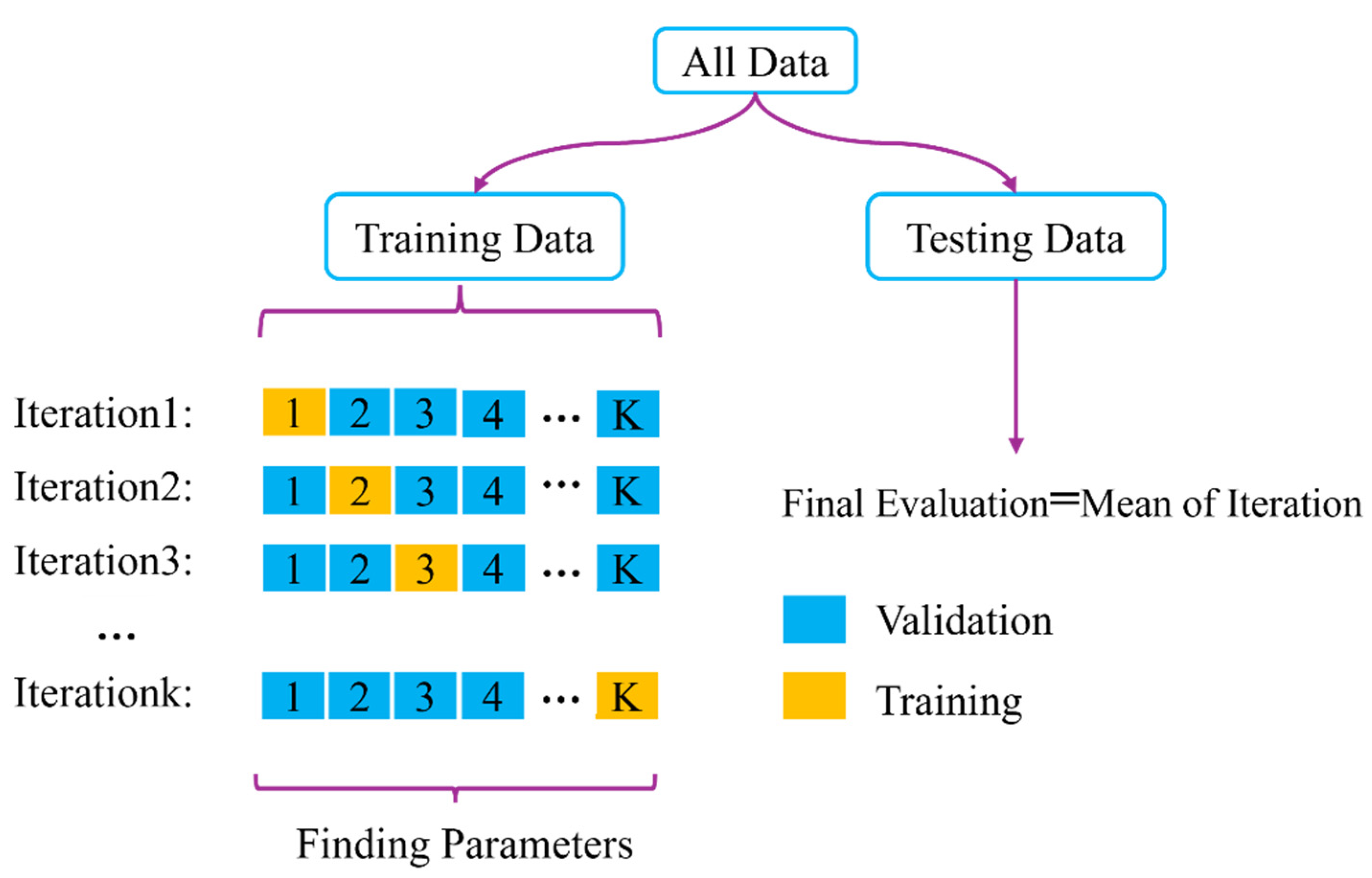
In this experiment, to fully utilize all the data for both training and validation, and to ensure the improved model maintains robust performance under different data splits, a five-fold cross-validation method was chosen. This method divides the data into 5 equal-sized subsets, using one of them as the validation set and the remaining 4 as the training set. The process is repeated 5 times. The final evaluation of the experiment is based on the average of the 5 results. The diagram illustrating the experimental process is shown in Figure 24 below.

In this study, a cross-validation experiment was conducted using measured datasets and public datasets. The data were randomly divided into five subsets, each containing 877 samples. In each iteration, one subset served as the validation dataset while the remaining four were used as the training dataset, with the process repeated five times. The purpose was to evaluate the predictive performance of the model on different datasets or unseen data, thereby demonstrating that the experimental results are not coincidental. According to the principle of five-fold cross-validation, the experimental results of the improved model in this study, Informer-SEnet, are presented in the following

Table 5. Cross-validation results of Informer-SEnet (the proposed method in this paper).

Iteration Number	Measured Dataset 1			Measured Dataset 2			Open Dataset
	MAE	RMSE	R2	MAE	RMSE	R2	MAE	RMSE	R2
1	1.515	1.202	0.985	1.836	1.478	0.970	2.091	1.648	0.964
2	1.442	1.140	0.985	1.632	1.264	0.962	1.960	1.540	0.976
3	1.692	1.355	0.980	2.482	1.952	0.981	2.146	1.681	0.966
4	1.346	1.050	0.988	2.202	1.750	0.986	1.994	1.580	0.968
5	1.501	1.221	0.983	1.991	1.571	0.987	1.943	1.523	0.972
Average	1.499	1.194	0.984	2.029	1.603	0.977	2.027	1.594	0.969
Standard Deviation	0.113	0.100	0.003	0.294	0.234	0.010	0.078	0.061	0.005

:

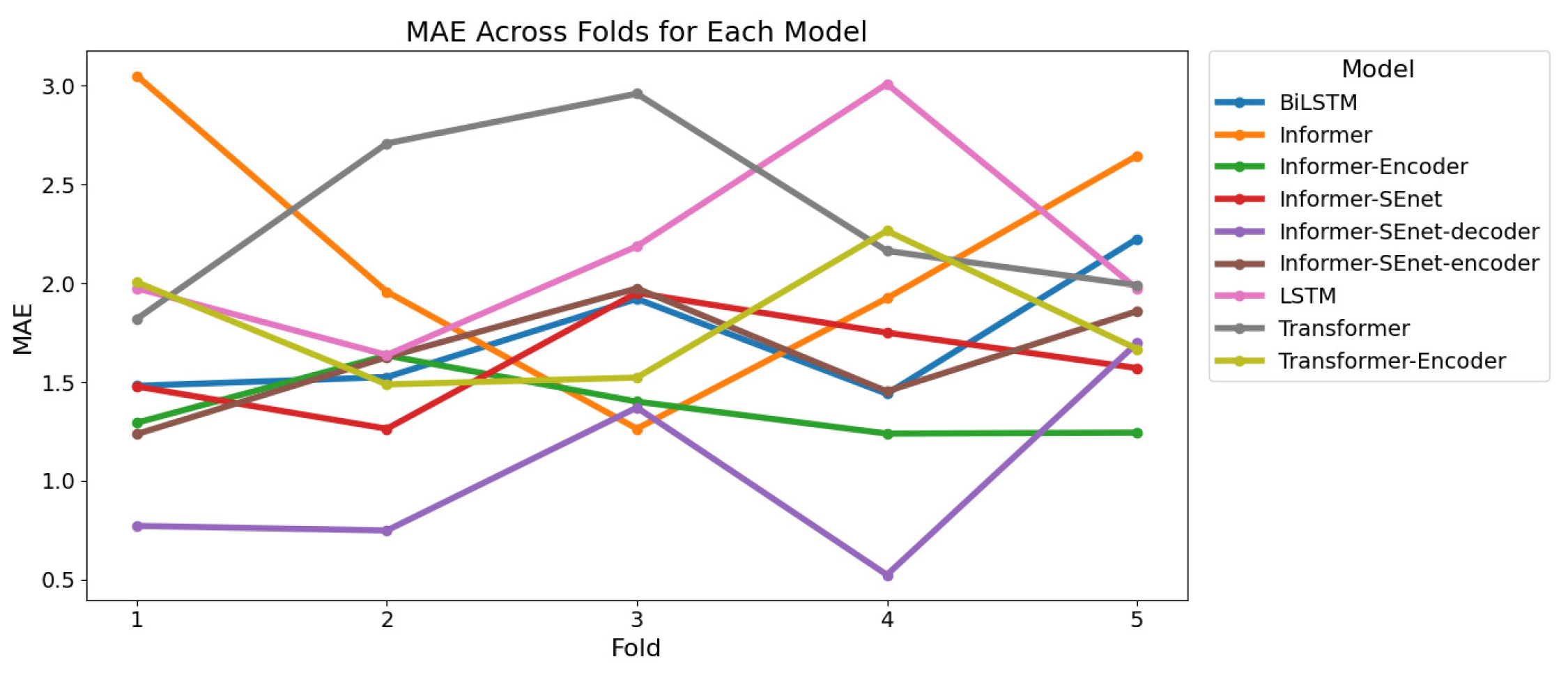
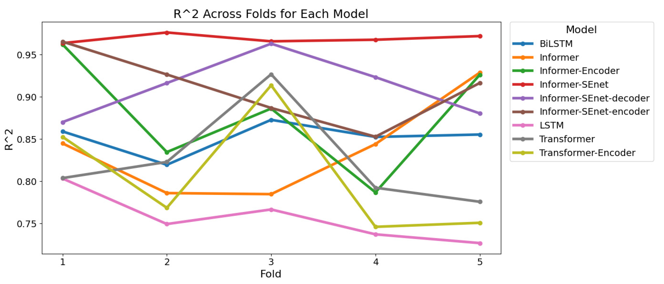
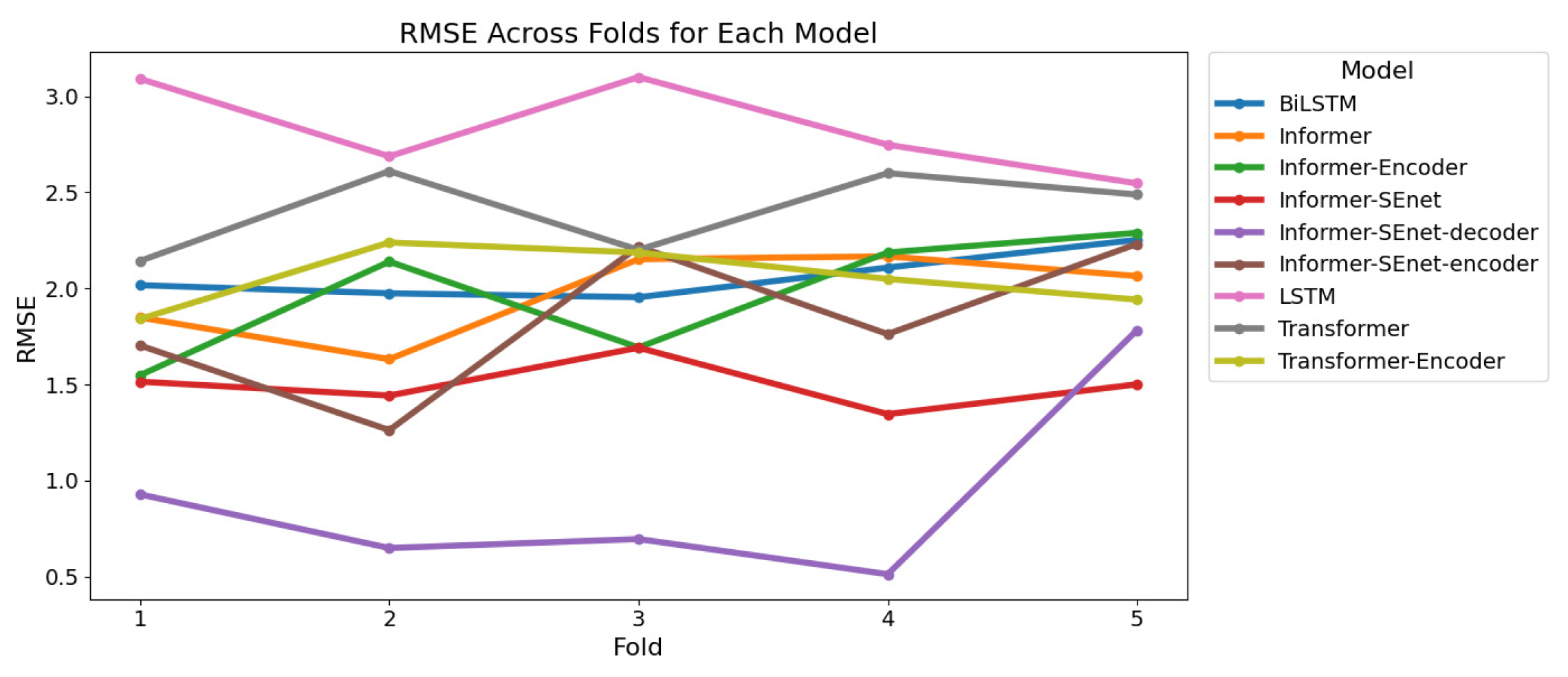
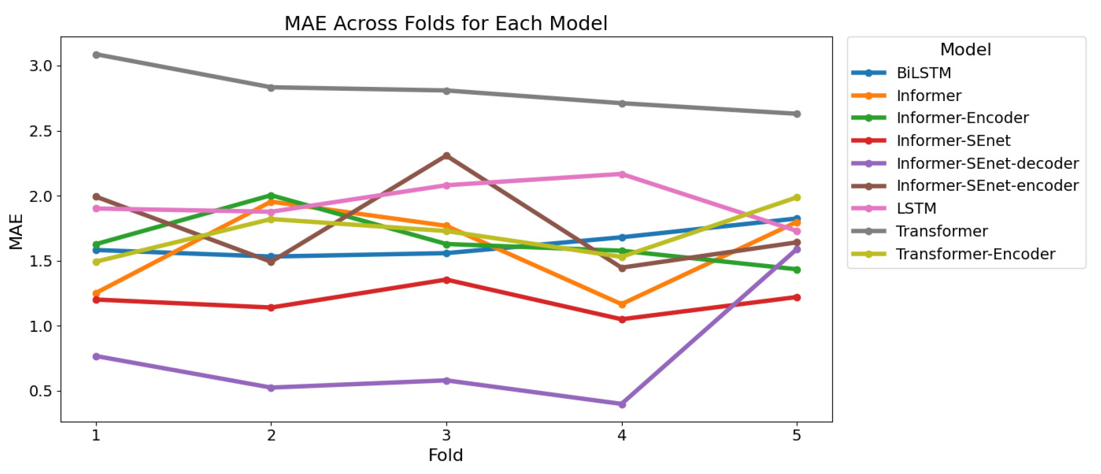
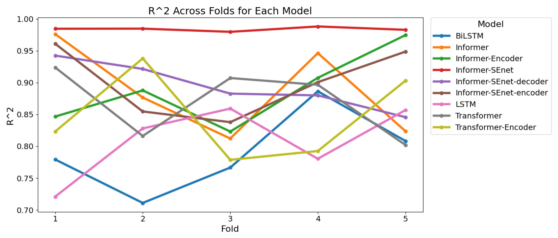
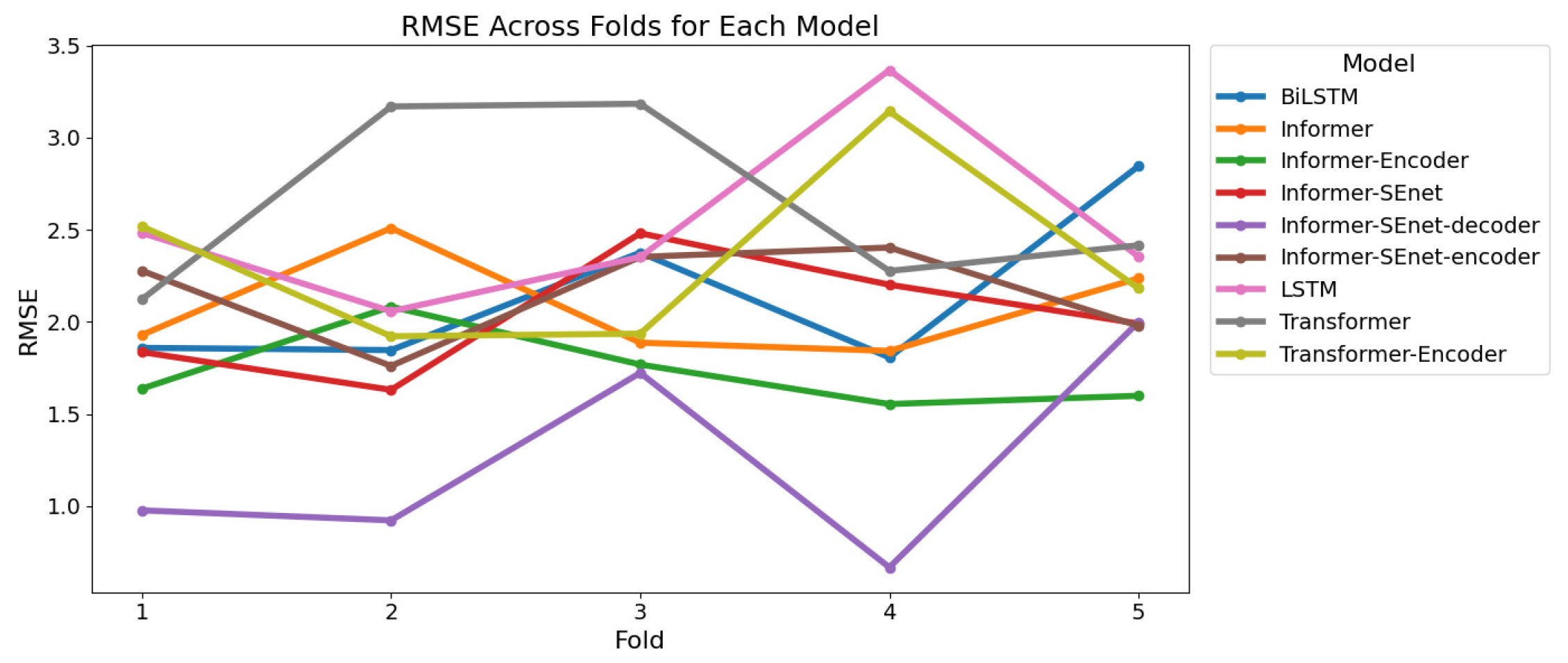
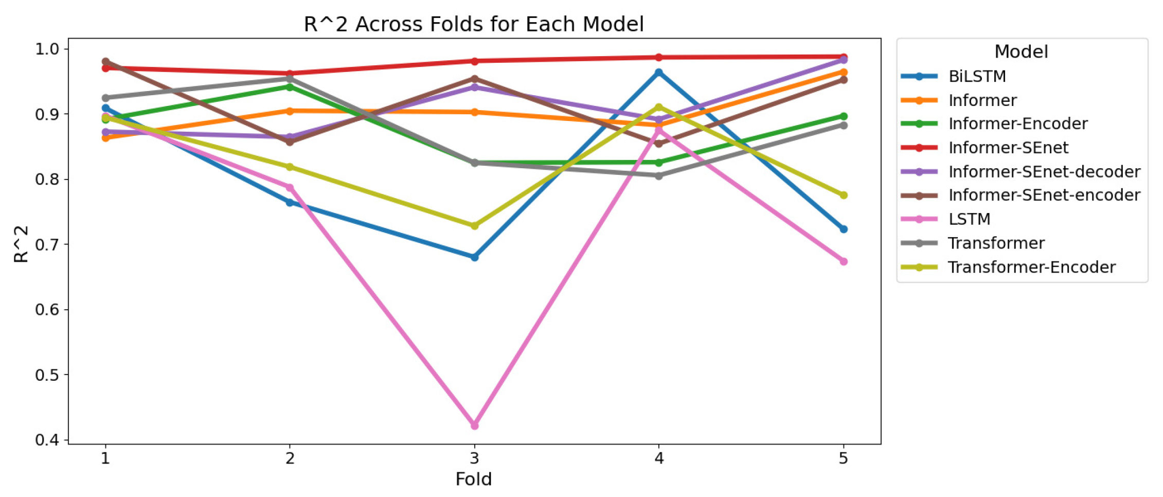
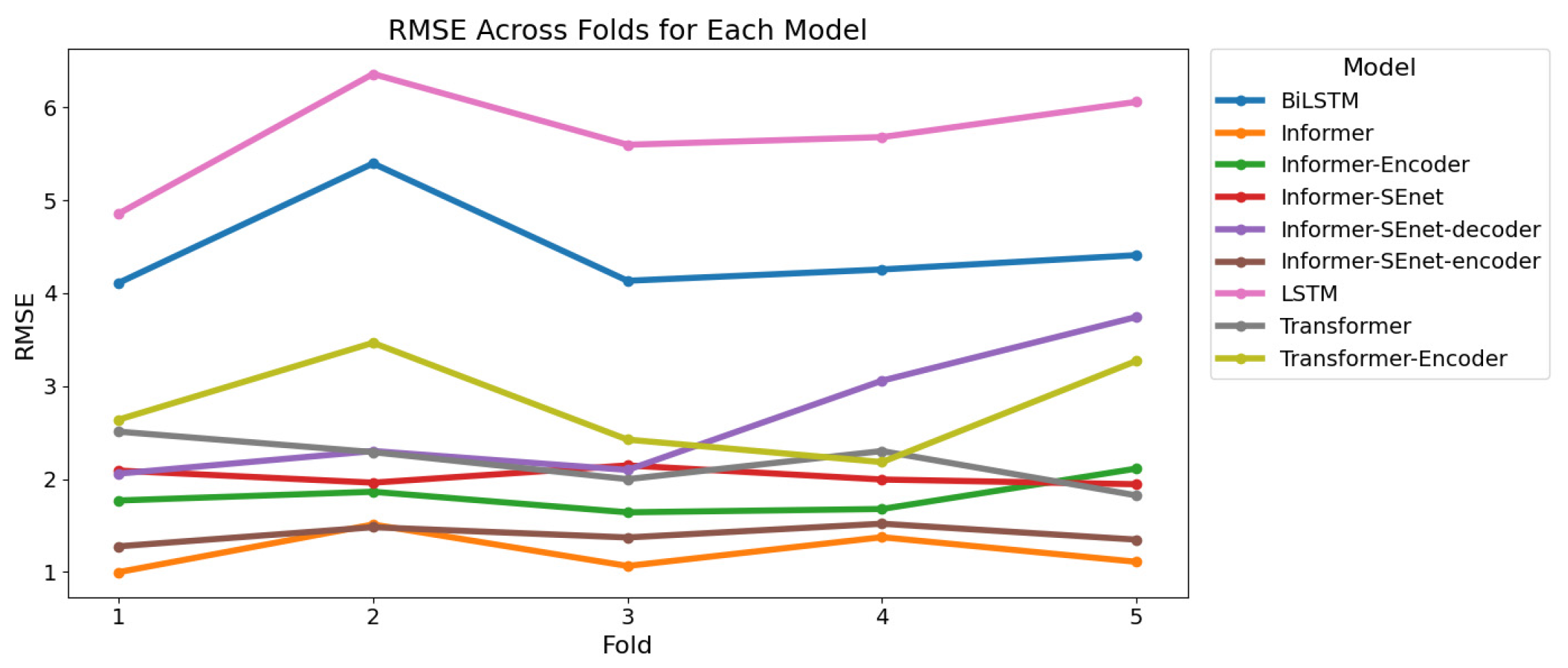
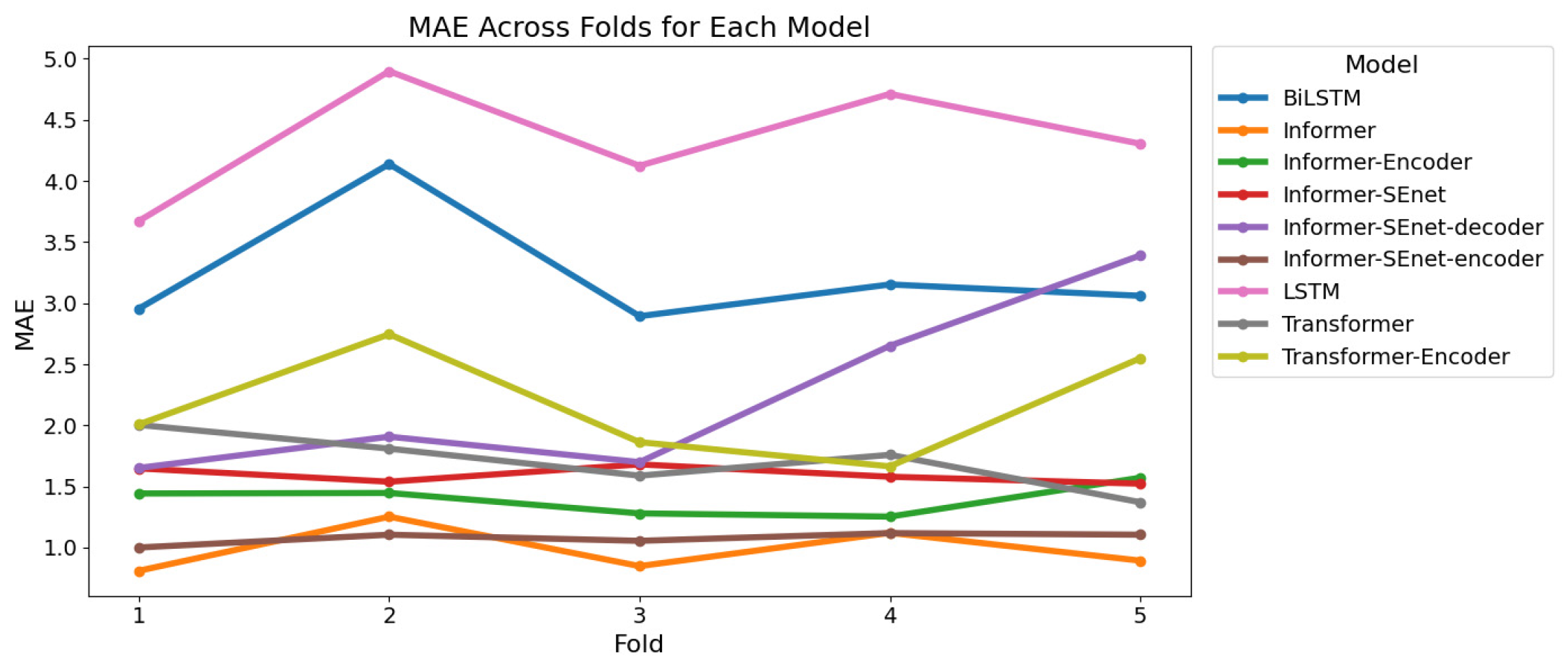
In addition, to further highlight the reliability and accuracy of the improved model proposed in this paper, a five-fold cross-validation experiment was also conducted on the baseline models. Given the large number of baseline models, representative models such as LSTM and Informer were selected as the control experimental groups. Their results are shown in Figure 25, Figure 26, Figure 27, Figure 28, Figure 29, Figure 30, Figure 31, Figure 32 and Figure 33 below.

To evaluate the robustness and reliability of the proposed Informer-SEnet model in structural response prediction tasks, this study employed a five-fold cross-validation method for experimental validation. In each experiment, Informer-SEnet was compared with the other six baseline models (including LSTM, BiLSTM, Transformer, and its variants) under the same training–validation split. Through five complete iterative experiments, the RMSE, MAE, and R² metrics were calculated for the test set of each fold.

The experimental results show that the proposed Informer-SEnet model demonstrated superior and stable performance across all metrics in the five-fold validation. Its average RMSE and MAE were the lowest among all compared models, and the corresponding standard deviations were generally smaller than those of other models. This indicates that the model’s predictions exhibit smaller fluctuations and possess good adaptability to different data partitions. In contrast, although some baseline models performed adequately in certain folds, their metric standard deviations were relatively larger, indicating that their performance is more susceptible to variations in training data distribution and that their robustness is inferior to the proposed model.

In summary, the five-fold cross-validation results statistically confirm that Informer-SEnet not only significantly outperforms the selected baseline models in prediction accuracy but also exhibits better robustness and generalization capability. This further supports the reliability of the proposed model for practical applications in engineering time-series prediction.

5. Conclusions

The chapter proposes a multivariate long-term structural response prediction method based on Informer-SEnet, and the main conclusions are as follows:

(1) To address the characteristics of multivariate structural response sequences, such as strong nonlinearity, significant long-term dependencies, and complex feature coupling, this chapter constructs a deep learning model that combines the long-sequence modeling capability of Informer with the channel attention mechanism of SEnet. The SE module can adaptively adjust the importance of different feature channels, enhancing the representation of key structural response physical quantities (e.g., temperature, strain) and thereby effectively improving the model’s feature extraction capability in multi-source coupled monitoring data.

(2) The chapter introduces targeted optimizations to the original Informer architecture: incorporating a sparse attention mechanism to reduce computational burden in long sequences; utilizing convolutional pooling to enhance multi-scale feature extraction; and integrating channel recalibration mechanisms into the encoder and decoder to improve feature representation effectiveness and overall model stability. These improvements work synergistically, enabling the model to more fully capture long-term trends and periodic features of structural responses and enhancing its adaptability to complex, non-stationary sequences.

(3) Comparative experiments based on monitoring data from two actual bridges and publicly available datasets demonstrate that Informer-SEnet significantly outperforms traditional RNN-based models (e.g., LSTM, BiLSTM) and certain Transformer variants in terms of prediction stability and generalization capability. Further ablation experiments validate the effectiveness of the sparse attention, convolutional pooling, and channel attention modules. Additionally, five-fold cross-validation results show that the model maintains consistent performance improvements under different data partitioning conditions, with smaller fluctuations in MAE, RMSE, and R² compared to baseline models, indicating good robustness and generalizability.

(4) From a structural engineering perspective, the improvement in prediction accuracy and stability of structural responses holds significant engineering implications: high-quality predictions of response trends over the next 24 h enable more timely and reliable identification of abnormal structural changes, reducing false alarms and missed detections, and enhancing the scientific basis for early warning threshold settings. Simultaneously, advance prediction provides maintenance departments with sufficient intervention windows, facilitating preventive maintenance, traffic organization adjustments, or risk assessments, thereby supporting decision-making for the long-term safe operation of bridges. In summary, the Informer-SEnet model proposed in this chapter provides an efficient, robust, and engineering-applicable method for long-term response prediction and intelligent early warning in bridge structural health monitoring.