Comparative Study on Internal and External Damage Imaging Using Ultrasonic Guided Waves Within a Variational Bayesian PCA Framework

Abstract

This study presents a comparative analysis of the novel guided-wave-based imaging method that integrates variational Bayesian principal component analysis with time-delay strategy for detecting internal and external defects in plate-like structures. The performance of the conventional delay-and-sum imaging method deteriorates when the signal-to-noise ratio of signals is low or when other wave packets overlap with the defect scattering signal. The imaging method based on variational Bayesian principal component analysis analyzes the principal components and corresponding singular values of the time-delayed signal array, and the maximum singular value represents the contribution of the most principal component, serving as an indicator of the coherent defect-related wave packets. Thus, the defect can be highlighted by accounting for the effect of noise and wave packet interference on the time-delayed signal array. However, when defects are located outside the sensor network, the limited information available may reduce the imaging performance. Numerical simulations and experimental studies conducted on plate-like structures demonstrate the proposed method achieves higher imaging clarity and localization accuracy for the internal defect compared with the external defect, with the former exhibiting mm-level absolute localization errors.

1. Introduction

Over the past few decades, metal thin-plates have been widely used in building construction to reduce structural weight and enhance load bearing capacity, such as the orthotropic steel decks in bridges, and steel plate-concrete composite walls in high buildings. However, these plate-like structures in service are susceptible to corrosion, cracking, impact, etc. These damages gradually develop and eventually compromise structural safety. Implementing real-time non-destructive testing is essential to ensure the integrity and reliability of these structures [1]. Among the available non-destructive testing methods, the guided wave detection technique has been extensively applied due to its high sensitivity to minor defects [2], wide inspection area [3], and economic feasibility [4]. Nevertheless, guided wave signals are difficult to interpret because of multiple modes, mode conversion and dispersion [5]. To address these challenges, two main research approaches have been developed. The first focuses on utilizing non-dispersive guided wave modes to reduce the signal complexity [6], while the second aims to employ the imaging methods to simplify signal processing, including delay-and-sum (DAS) [7], the reverse time migration method and its improvements [8,9], multiple signal classification algorithm [10], tomography [11], a reconstruction algorithm for probabilistic inspection of damage algorithm [12], unsupervised data-driven method [13], deep-learning-assisted localization algorithm [14], etc.

These aforementioned imaging methods are deterministic without considering uncertainty during defect localization, including the measurement noise [15], the imprecise group velocity of the employed Lamb mode [16], and the inherent limitations of signal processing [17], etc. To quantify the uncertainty, Khurjekar et al. [18] proposed a mixture density network to generate the probabilistic distribution of the damage location based on the training data. Subsequently, they developed a deep learning framework for estimating uncertainty in damage identification [19]. Lu et al. [20] proposed an uncertainty quantification framework based on Flipout probabilistic convolutional neural network, which separates uncertainty in guided-wave-based detection into aleatoric and epistemic components. Zhang et al. [21] proposed a Bayesian method fusing the time-of-flight and damage index of the valid path to improve the stability and robustness of localizing results. Hu et al. [22] proposed a hierarchical hyper-Laplacian prior in the Bayesian framework to localize corrosion defects in pipes. Another important means for uncertainty quantification is the Bayesian approach, which can make full use of the collected data and prior knowledge to derive the posterior probability density function of unknown parameters within the approximate physical model [23,24]. Yue and Aliabadi [25] proposed a novel hierarchical Bayesian approach to estimate the uncertainty of damage sensitive features, providing a rational basis for setting a reasonable threshold to achieve reliable location of damage. Xue et al. [26] employed multitask complex hierarchical sparse Bayesian learning to infer the dispersion curves of guided waves and optimize the sensor placement. Wu et al. [27,28] utilized sparse Bayesian learning to reconstruct multiple dispersive Lamb modes from the received signals and identify the wave packet features via a Gabor pulse model. Song and Yang [29] proposed a Bayesian deep learning approach to quantify and interpret various uncertainties in super-resolution guided wave array imaging. These studies demonstrate that the Bayesian approach can be introduced to guided-wave-based damage detection to improve the identification performance by considering uncertainty.

Among various imaging techniques, the DAS method is widely adopted due to its simplicity, flexibility in sensor placement, and robust imaging performance [30]. The pixel value of the DAS imaging method is obtained by summing the amplitudes of all time-delayed signals at the reference time-of-flight (ToF). However, when applied to small or complex structures, the pixel value may change due to wave packet overlapping or phase cancelation, thereby degrading imaging quality unless the first wave packet is accurately captured. Hence, a hybrid method of DAS imaging and variational Bayesian principal component analysis (VBPCA) is proposed to improve the resolution and contrast of guided-wave-based defect recognition [31]. VBPCA-based imaging method utilizes the maximum singular value of the principal components extracted from the time-delayed signal array as an indicator of defect, because the principal component associated with the largest singular value corresponds to the coherent defect scattering wave packet, thereby enabling effective suppression of complex wave packet interference, measurement noise, and other backgrounds. In addition, this method only requires multi-point time-series wavefield measurements, which can be realized using adhesive-bonded and non-contact sensing technologies, and then this method is a generalizable signal-decomposition and feature-separation framework that can be integrated with a wide range of sensing schemes. In contrast to the DAS imaging method, which captures local features, the VBPCA-based imaging method focuses on the characteristics of the entire reflected wave packet, offering a more detailed representation of the guided wave signal. Thus, this method demonstrates excellent imaging performance for the defects located within the sensor network. Nevertheless, the limited defect information available when the defect is located outside the sensor network may restrict the effectiveness of the VBPCA-based imaging method, thereby motivating the present study.

The remainder of this paper is organized as follows. Section 2 briefly introduces the conventional DAS and VBPCA-based imaging algorithms for defect detection in the plate-like structures. Section 3 validates the performance of these two imaging methods using numerical simulation, including cases where defects are located both inside and outside the sensor network. Section 4 presents an experimental study to further validate the proposed method under both conditions. Finally, the conclusions are summarized in Section 5.

2. Materials and Methods

The DAS imaging method localizes the damage by delaying all signals according to the ToF differences in ultrasonic guided wave signals propagating along all transmitter-position-receiver paths, as shown in Figure 1, and then summing the Hilbert transform coefficients [32] of the time-delayed signals based on the ToF of the reference transmitter–position–receiver path. The ToF difference corresponds to the distance difference divided by group velocity, which can be expressed as:

$$\begin{array}{c}{∆t}_{h,g}={\displaystyle \frac{∆s_{h,g}}{v}}={\displaystyle \frac{\sqrt{{\left(x_h^t-x_g\right)}^2+{\left(y_h^t-y_g\right)}^2}+\sqrt{{\left(x_h^r-x_g\right)}^2+{\left(y_h^r-y_g\right)}^2}}{v}}\\ -\underset{h}{\min }\left({\displaystyle \frac{\sqrt{{\left(x_h^t-x_g\right)}^2+{\left(y_h^t-y_g\right)}^2}+\sqrt{{\left(x_h^r-x_g\right)}^2+{\left(y_h^r-y_g\right)}^2}}{v}}\right)\end{array}$$

(1)

where v represents the group velocity of the used Lamb mode; $\left(x_h^t,{ y}_h^t\right)$ and $\left(x_h^r,{ y}_h^r\right)$ are the coordinates of transmitter and receiver sensors in the h-th transmitter–receiver pair, respectively; (x_g, y_g) is the coordinate of the g-th position. However, the DAS imaging method directly sums the time-delayed array and is therefore sensitive to overlapping wave packets and noise.

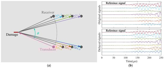
Figure 1. Diagram of time-delay strategy: (a) the locations of sensors and a crack located outside the sensor network; (b) original signals and the time-delayed signals. The gray dashed lines denote Hilbert transform coefficients.

Instead of using the average amplitude of the time-delayed arrivals as the pixel value, the VBPCA-based imaging approach [31] employs the maximum singular value associated with the principal component of each time-delayed signal array, as shown in Figure 2. The process begins by applying a smoothing rectangular window with a length of the excitation pulse to segment the time-delayed residual signals into multiple subarrays, as shown in Figure 2b. Each residual signal in the column of the subarray is normalized. Subsequently, a phase coherence factor is applied to each row of the normalized subarray to reduce the amplitude of the signals with poor phase consistency [33], which can be expressed as:

$$\mathrm{P}\mathrm{C}\mathrm{F}\left(t_c\right)={\displaystyle \frac{1}{\mathrm{V}\mathrm{a}\mathrm{r}\left({\phi }_1\left(t_c\right),{\phi }_2\left(t_c\right),\dots ,{\phi }_h\left(t_c\right)\right)}}$$

(2)

where PCF is the phase coherence factor at the corresponding time $t_c$, ${\phi }_1\left(t_c\right),{\phi }_2\left(t_c\right),\dots ,{\phi }_h\left(t_c\right)$ represent the phases of the residual signals at the corresponding time $t_c$, and $\mathrm{V}\mathrm{a}\mathrm{r}\left(·\right)$ denotes the variance of these phases. After phase correction, the VBPCA algorithm decomposes the preprocessed subarray into low-rank and sparse components, which can be expressed as follows:

$$\mathbf{Y}=\mathbf{X}+\mathbf{S}+\mathbf{N}$$

(3)

where Y is the preprocessed subarray; X is the low-rank component matrix, corresponding to coherent wave packets; S is the sparse noise matrix; and N is the normal noise matrix. The low-rank component matrix X is further factorized into A and B, which share the same sparsity profile and are governed by a hierarchical prior structure, consisting of a zero-mean Gaussian prior in the inner layer and a Gamma hyperprior in the outer layer that controls the inverse variance of the Gaussian prior. In the following studies, the shape and scale parameters of this Gamma hyperprior are set as 10⁻⁵. The sparse noise matrix adopts the hierarchical prior that combines zero-mean Gaussian prior with noninformative Jeffreys hyperprior to govern the inverse variance of the Gaussian prior, and the initial value of the Jeffreys parameter is set to the root mean square of the subarray Y. The normal noise matrix is also employed the same hierarchical prior structure, with the initial Jeffreys parameter set to the mean square of the subarray Y. And then the posterior probability distributions of these matrices can be derived [31]. The VBPCA algorithm iteratively estimates the posterior distributions of the principal components, under a hierarchical Bayesian framework until convergence. The convergence criterion is defined by $‖{\mathbf{X}}^p-\mathbf{X}‖/‖\mathbf{X}‖<{10}^{-5}$, where ${\mathbf{X}}^p$ denotes the result from the previous iteration. The singular values associated with these principal components are then extracted, and the largest singular value representing the dominant defect scattering wave packets is used as the primary indicator of defect presence. In addition, the sum of the maximum singular values of the subarrays centered at the reference ToF is finally adopted as the pixel value at each spatial position. This VBPCA-based imaging method effectively separates coherent, defect-induced responses from overlapping wave packets and measurement noise. As a result, VBPCA algorithm provides a clearer distinction between defect and undamaged positions, yielding higher imaging resolution and contrast.

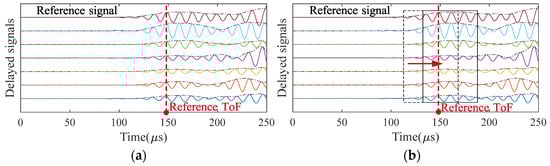
Figure 2. Comparison of imaging principles between: (a) the conventional DAS imaging method; (b) the VBPCA-based imaging method. The dashed and solid rectangular boxes indicate the smoothing rectangular window, and the red dashed lines denote the locations of the reference ToF.

3. Numerical Studies

3.1. Setup of Numerical Simulations

To study the effectiveness of VBPCA used for defect imaging, ultrasonic guided wave signals reflected from a crack in a plate with free boundary conditions obtained by ANSYS software (version 18.0) simulation were first imaged. The plate has a length of 1 m, a width of 0.6 m, and a thickness of 0.12 m, as shown in Figure 3. The material of this plate is steel with a density of 7890 kg/m³, an elastic modulus of 209 G Pa, and Poisson’s ratio of 0.269. Based on these properties of this steel plate, the propagation velocities of transverse wave and longitudinal wave in isotropic media can be calculated as 3200 m/s and 5790 m/s according to the theoretical equations in [34], respectively. The center frequency of the employed five-cycle Hanning-windowed sinusoidal signal without noise is 70 kHz, and the amplitude of this excitation signal is 10 V. Therefore, the propagation velocity of S₀ mode was 5216 m/s based on theoretical dispersion curves [34] when the thickness of the plate was 12 mm.

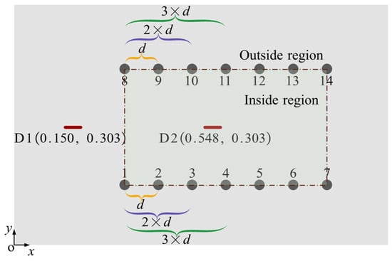
Figure 3. The locations of sensors and the cracks inside and outside the sensor network (unit: m). The short red lines are cracks, and the gray dots denote the sensors.

Figure 3 shows the locations of cracks and sensors in numerical simulations, in which the gray squares represent piezoelectric lead zirconate titanate (PZT) sensors. PZT can provide stable excitation and high-quality measured signals, allowing the performance of the proposed algorithm to be evaluated with precision and confidence. In addition, the wavefield data can also be acquired using non-contact techniques such as laser Doppler vibrometers, which provide flexible and high-resolution surface vibration measurements. Table 1 exhibits the locations of PZT sensors, whose physical properties are identical to those reported in [35]. There are 14 sensors in total, and each sensor acts as an exciter in turn, and the remaining sensors act as receivers; thus, there are 91 transducer pairs. To assess the identification performance of the VBPCA-based imaging method under various operating conditions, two representative cases were examined. Case 1 corresponds to crack D1 situated outside the sensor network, and Case 2 involves crack D2 located within the sensor network. Specifically, D1 and D2 are cracks that do not occur simultaneously. The center positions of D1 and D2 are (0.150, 0.303) m and (0.548, 0.303) m, respectively. And the size of each crack is 0.021 m in length, 0.003 m in width, and 0.009 m in depth.

Table 1. The sensor locations relative to the coordinate origin shown in Figure 3 (unit: m).

Number	Location	Number	Location
1	(0.360, 0.225)	8	(0.360, 0.375)
2	(0.435, 0.225)	9	(0.435, 0.375)
3	(0.510, 0.225)	10	(0.510, 0.375)
4	(0.585, 0.225)	11	(0.585, 0.375)
5	(0.660, 0.225)	12	(0.660, 0.375)
6	(0.735, 0.225)	13	(0.735, 0.375)
7	(0.810, 0.225)	14	(0.810, 0.375)

Firstly, baseline signals are obtained in a plate without defect. Secondly, unhealthy signals reflected from the defect in each condition are received to study the imaging performance. By subtracting the baseline signal from the corresponding unhealthy signal, the residual signal only related to the defect is obtained. Finally, all residual signals are processed by the conventional DAS and VBPCA-based imaging methods to localize the defect.

3.2. Defect Imaging Results and Analysis Based on Numerical Signals

Because multiple reflections and Lamb modes in the residual signals often overlap, the amplitudes at undamaged locations can exceed that at the crack location based on the DAS method, as shown in Figure 4. In addition, the amplitude canceling caused by the phase misalignment also affects the imaging effect. Therefore, the first wave packet in residual signal is roughly isolated by applying a rectangular window with its start point determined by a specified threshold indicating a sudden amplitude increase and its length corresponding to the excitation signal duration. The Hilbert coefficients outside this window are set to zero. And then all isolated first wave packets are used to image the defect.

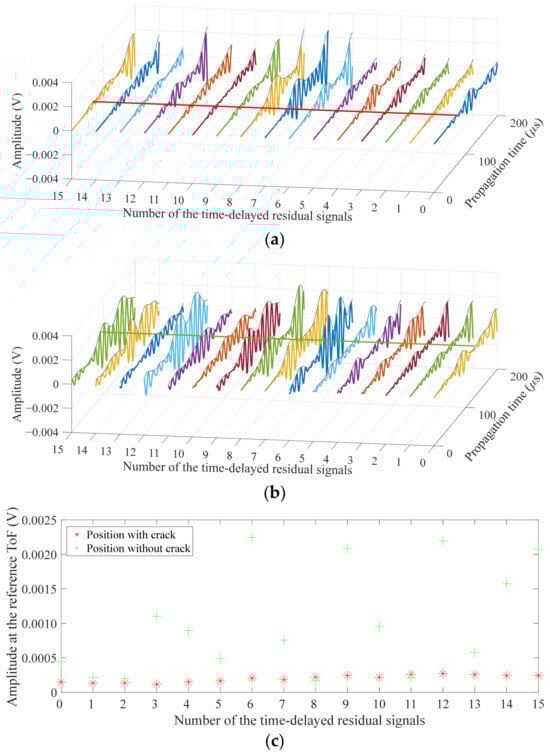
Figure 4. Amplitudes of time-delayed signals: (a) signals focused on the position with crack; (b) signals focused on position without crack; (c) comparison of the amplitudes at the reference ToF.

Figure 5 illustrates D1 and D2 imaging results obtained by the conventional DAS method using the entire signals and the first wave packets. When the entire signals are utilized, the defect location cannot be clearly identified. This is primarily because the Hilbert coefficient of the subsequent wave arrivals may exceed that of the first defect scattering wave packet. At the defect grid, although the selected coefficients are all related to the defect scattering wave packet, these Hilbert coefficients are very small, as shown in Figure 4, causing the superposed coefficient at defect position to be smaller than those at undamaged regions. As a result, the location of the defect cannot actually be highlighted. Figure 5c,d presents the conventional DAS imaging results utilizing the first wave packets of all residual signals. It can be observed that utilizing the first wave packets enables a rough identification of defects D1 and D2. However, relatively large highlighted regions remain around the defect areas, indicating limited localization accuracy. The main reason is that some of the first wave packets still overlap with subsequent arrivals, which increases the superposed amplitude. Moreover, the imaging quality is highly sensitive to the threshold employed to determine the start point of the first wave packet.

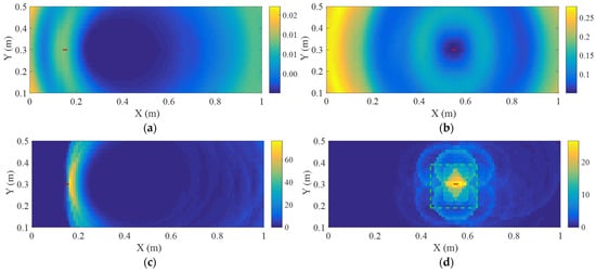
Figure 5. DAS imaging results based on Hilbert coefficients: (a) D1 image using the entire signals; (b) D2 image using the entire signals; (c) D1 image using the first wave packets; (d) D2 image using the first wave packets. Red lines denote cracks, and green dashed box indicates the identified region used to calculate the contrast.

To improve the resolution and contrast of defect imaging, the VBPCA algorithm is employed to process the time-delayed signal array. When each signal in some windowed subarray contains too many small amplitudes, as shown in the left dotted black window in Figure 2, it indicates that no complete defect scattering wave packet is present. In such cases, the pixel value of the corresponding gird is set to zero. Figure 6 presents the imaging results of D1 and D2 using VBPCA-based imaging method. It can be found that this method effectively reduces the region of defect and then obviously highlights the defect, thereby improving the efficiency and accuracy of defect localization. The identified D1 and D2 are almost perfectly consistent with the actual defects, for example, the identified location of internal defect is (0.55, 0.30) m with a posterior variance of 10⁻¹², indicating an extremely high level of confidence. Table 2 presents the absolute errors obtained by five methods for internal defect imaging, which validates the effectiveness of the proposed method. In addition, the resolution of D2 located within the sensor network is much better than that of D1, which is outside the sensor network. This difference arises because the sensor network surrounding D2 provides more comprehensive information, effectively constraining the defect boundary, whereas the unilateral sensor configuration near D1 refines only the boundary on the sensor side. Therefore, for external defect, the absolute error is defined as the distance from the identified location to the nearest defect boundary, whereas for internal defect, it is defined as the distance between the identified location and the defect center. Four defect lengths are considered to investigate the influence of defect length on the imaging performance of the proposed method. The internal defect imaging results obtained by DAS and VBPCA-based methods are presented in Figure 7 and Figure 8, and the absolute errors for defects with different lengths are shown in Figure 9. These absolute errors exhibit strong stability, and the errors of internal defects are slightly smaller than those of some external defects. Consequently, the VBPCA-based imaging method is more effective for the defects inside the sensor network.

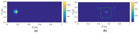
Figure 6. Defect imaging results based on VBPCA-based imaging method: (a) D1; (b) D2. Red lines denote cracks, and green dashed box indicates the identified region used to calculate the contrast.

Table 2. Comparison of absolute errors obtained by five methods for internal defect imaging.

Unsupervised Data-Driven Method [13]	Deep-Learning-Assisted Localization Method [14]	Bayesian Fusion Method [21]	Bayesian Framework with Hierarchical Priors [22]	The Proposed Method
0.008 m	0.007 m	0.007 m	0.0008 m	0.004 m

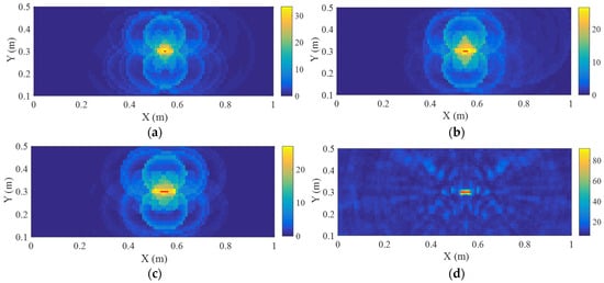
Figure 7. D2 imaging results based on DAS method for four lengths: (a) 0.009 m; (b) 0.021 m; (c) 0.033 m; (d) 0.045 m. Red lines denote cracks.

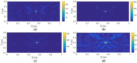
Figure 8. D2 imaging results based on VBPCA-based method for four lengths: (a) 0.009 m; (b) 0.021 m; (c) 0.033 m; (d) 0.045 m. Red lines denote cracks.

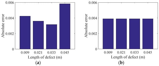
Figure 9. Absolute errors for defects with different lengths based on VBPCA-based imaging method: (a) D1; (b) D2.

The contrast ratios of the identified regions enclosed by green dotted lines in Figure 5d and Figure 6b, defined as the standard deviation of pixel intensities divided by their mean, are 0.64 and 1.97 for the DAS and VBPCA-based imaging results, respectively, demonstrating the significantly enhanced clarity achieved by the proposed method. In addition, the imaging results obtained from sensor networks with different sensor spacings are shown in Figure 10. Compared with the imaging results in Figure 6b, it can be observed that sensor spacing has minimal influence on imaging accuracy.

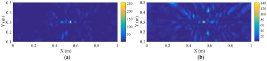
Figure 10. Internal defect imaging results using sensor subsets to obtain sensor spacings of: (a) 2 × d; (b) 3 × d. Red lines denote cracks.

The VBPCA-based imaging method requires approximately 0.02 s to process the time-delayed subarray focused on each position, as illustrated in Figure 11, which is considered acceptable for engineering applications. Figure 12 shows the number of iterations required for convergence. Typically, about 100 iterations are needed to process the numerical signals.

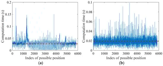
Figure 11. Computation time of VBPCA-based imaging method: (a) D1; (b) D2. Red dashed line in each subfigure denotes the mean value of the data.

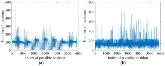
Figure 12. Number of iterations of VBPCA-based imaging method: (a) D1; (b) D2. Red dashed line in each subfigure denotes the mean value of the data.

4. Experimental Studies

4.1. Setup of the Experiment

To further validate the performance of the VBPCA-based imaging method, an experimental test was conducted under laboratory conditions, in which a bolt bonded to an aluminum plate was used to simulate a defect. The material of this plate was Aluminum 6061-T6, with a density of 2700 kg/m³, an elastic modulus of 70 G Pa, and Poisson’s ratio of 0.33. Based on these parameters, the theoretical longitudinal and transverse wave velocities were calculated as 6198 m/s and 3122 m/s, respectively. Considering the plate thickness of 4 mm and an excitation center frequency of 200 kHz, the group velocity of the employed S₀ mode was determined to be 5288 m/s.

Figure 13 presents the layout of PZTs marked by blue circles and the defect marked by a red asterisk, whose center location is (0.61, 0.59) m. Twenty circular PZTs were utilized to investigate the case where the defect was located inside the sensor network. Table 3 lists all PZT locations relative to the coordinate origin. Each PZT had a diameter of 7 mm and a thickness of 1 mm. In this setup, each PZT sequentially acted as an exciter while the remaining PZTs acted as receivers, resulting in a total of 190 transducer pairs. For the case where the defect was located outside the sensor network, only the first ten PZT sensors numbered 1 to 10 were utilized, and then there were 45 transducer pairs in total.

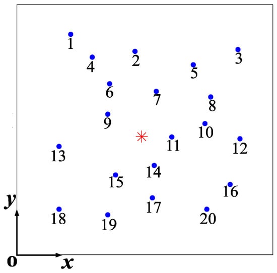
Figure 13. The layout of PZT sensors and the defect in the experimental studies. Red asterisk (*) denotes the defect, and blue dots are sensors.

Table 3. The PZT locations relative to the coordinate origin shown in Figure 13 (unit: m).

Number	Location	Number	Location
1	(0.264, 1.100)	11	(0.758, 0.587)
2	(0.578, 1.015)	12	(1.091, 0.578)
3	(1.081, 1.024)	13	(0.207, 0.540)
4	(0.369, 0.986)	14	(0.672, 0.445)
5	(0.863, 0.948)	15	(0.483, 0.397)
6	(0.454, 0.853)	16	(1.043, 0.350)
7	(0.682, 0.815)	17	(0.663, 0.283)
8	(0.948, 0.787)	18	(0.207, 0.226)
9	(0.445, 0.701)	19	(0.445, 0.198)
10	(0.920, 0.654)	20	(0.929, 0.226)

An arbitrary waveform generator (Tektronix, Beaverton, OR, USA, AFG3252), a power amplifier (Agitek, Xi’an, China, ATA-6610) and an oscilloscope (Tektronix, USA, DPO2004B) were employed to generate, magnify and record the guided wave signals, respectively. Baseline and unhealthy signals were received by each PZT and then subtracted to obtain the corresponding defect scattering residual signal.

4.2. Defect Imaging Results and Analysis Based on Experimental Signals

Figure 14 shows the residual signals received by all transducer pairs when the defect is located outside the sensor network, and the signals for the case of inside defect are not presented here due to the large number of signals. As shown in Figure 15, the signal-to-noise ratio (SNR) of each residual signal is relatively low, making it difficult to clearly distinguish the wave packets from noise. Therefore, filtering is an indispensable preprocessing step. The wavelet coefficients of a residual signal are shown in Figure 16, where the red-boxed region, centering at the excitation frequency with a 200 kHz bandwidth, fully encompasses all wave packets. Then, each residual signal was subsequently filtered within this bandwidth to isolate the target frequency component from low-frequency noises, as indicated by the red waveform in Figure 14. Subsequently, both the conventional DAS and VBPCA-based imaging methods were employed to localize the defects located inside and outside the sensor network.

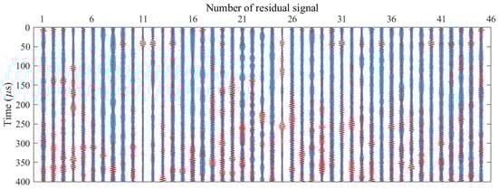
Figure 14. A comparison of the residual signals before and after filtering when the defect is located outside the sensor network.

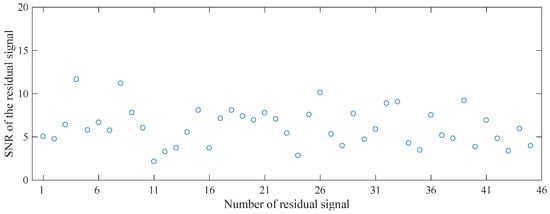
Figure 15. SNR of the residual signal when the defect is located outside the sensor network.

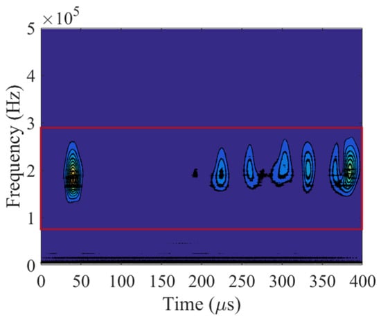
Figure 16. The wavelet coefficients of a residual signal. Red box denotes the bandpass filter.

Because the DAS method provides poor imaging performance when processing the entire signals in simulation studies, the first wave packets in these experimental residual signals are employed to identify the external and internal defect, as shown in Figure 17. It can be seen that the areas of defect identified by DAS imaging method are relatively large, as shown in the purple box that is circled by choosing the pixel value larger than a preset threshold. In addition, the area of the identified external defect is slightly larger than that of the identified internal defect, resulting from the limited defect information. And the locations of the largest pixel values for the external and internal defect identification are (0.64, 0.59) m and (0.61, 0.58) m, respectively. Compared with the actual defect position (0.61, 0.59) m, the absolute errors are 0.02 m from the defect boundary to the identified location and 0.01 m from the defect center to the identified location, where the performance of external defect imaging is inferior to that of internal defect imaging.

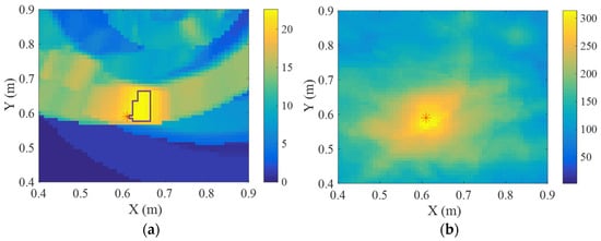
Figure 17. DAS imaging results based on Hilbert coefficients of the first wave packets: (a) external defect; (b) internal defect. Red asterisk (*) in each subfigure denotes the defect, and the purple box indicates the identified region with pixel values exceeding a preset threshold.

Figure 18 shows the imaging results of external and internal defects by using the VBPCA-based imaging method. Due to the small SNR of the residual signals, although the singular values of the defective and undamaged grids are not much different, it can still be clearly seen that the singular values of the defect grid are larger than those of undamaged grid. The identified region of the VBPCA-based imaging method becomes extremely small, as shown in Figure 18b. Specifically, the area ratio of the highlight regions circled by both methods is around 1:65 for identifying the external defect, which means the proposed method significantly simplifies the decision-making process for defect identification. The positions corresponding to the maximum pixel values obtained by the VBPCA-based imaging method for external and internal defects are (0.64, 0.59) m and (0.61, 0.58) m, respectively, with absolute errors of 0.02 m and 0.01 m. As same with the DAS imaging results, the performance of external defect imaging is also poorer than internal defect imaging. The inferior imaging performance of the proposed method for external defect identification is fundamentally attributed to the intrinsic scattering behavior of the S₀ mode. For external defect, the scattering angles of the S₀ mode are mainly distributed within the range of 20–120°, where the amplitudes of the scattered wave packets are relatively low, resulting in poorer imaging performance. In addition, the function of some sensors employed in this experiment is not good due to poor adhesion between sensor and plate, and then the corresponding residual signal exhibits wave packets with low amplitude, for instance, the 11th signal in Figure 14, which may adversely affect the imaging performance. But the VBPCA-based imaging method can still accurately identify the defect position, indicating its better performance than the DAS imaging method. It is worth noting that although the proposed method is demonstrated on a plate with an area of around 1.5 m², from a methodological perspective, it can be extended to larger structures when longer signal propagation times are recorded.

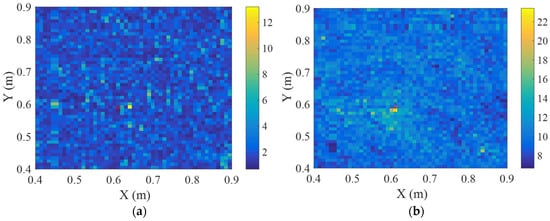
Figure 18. VBPCA-based imaging results of experimental signals: (a) external defect; (b) internal defect. Red asterisk (*) in each subfigure denotes the defect.

5. Conclusions

In this study, a hybrid method combining the time-delay strategy with variational Bayesian principal component analysis (VBPCA) is employed to identify defects located inside and outside the sensor network. When the received signals are time-delayed to focus on a defect, the damage scattering wave packets are highly coherent. As a result, the principal component extracted from the windowed subarray using the VBPCA algorithm predominantly represents the defect scattering wave packet, and its corresponding singular value is the largest. In contrast, when the wave packets are focused on a position without defect, the singular value is relatively small. Thus, the magnitude of the singular value can be used as an indicator for defect detection. By applying VBPCA to the time-delayed signal array, the strongly correlated principal component associated with the defect can be effectively extracted, while noise and interfering wave packets are suppressed, thereby enhancing the clarity and contrast of the imaging results.

The applicability of the VBPCA-based imaging method was first investigated using the guided wave signals obtained from numerical simulations of a steel plate containing defects. The conventional delay-and-sum (DAS) and VBPCA-based imaging methods were separately applied to localize the defects inside and outside sensor network. The comparison results indicate that the VBPCA-based imaging method effectively reduces the identified defect area, and the detected location coincides with the actual defect, meaning that the imaging clarity and localization accuracy are greatly improved. Furthermore, the highlight area corresponding to the internal defect is much smaller than that of the external defect, primarily because the internal defect is fully surrounded by sensors, allowing the whole boundary information to be captured, whereas only one-side information of the external defect is available to the unilateral sensor network. Another reason is that the scattering coefficients of the external defect are rather small, resulting in lower scattered wave packet amplitudes. Additionally, both imaging methods are applied to process the experimental signals obtained from an Aluminum plate. The imaging results indicate that the DAS and VBPCA-based imaging methods can identify the external defect with small absolute error of 0.02 m. This error sometimes arises from the large distance between the possible positions for rapid computation. This limitation can be addressed through a two-step discretizing strategy, which begins with a coarse grid for fast localization, followed by a second step that applies a much finer grid focused exclusively on the region identified in the first step, thereby reducing the absolute error by up to 0.01 m while maintaining computational efficiency. However, the area ratio of the identified regions is around 65:1, which demonstrates that the proposed method has better performance in the aspect of clarity. In addition, the absolute error of internal defect imaging is smaller than that of external defect imaging. Therefore, the VBPCA-based imaging method is more suitable for detecting defects located within the sensor network. Further investigations will be carried out to evaluate the performance of the proposed method for external and internal defects under specific engineering scenarios, such as identifying cracks in orthotropic steel bridge decks.

References

- Le, B.T.; Nguyen, T.T.; Truong, T.D.N.; Nguyen, C.T.; Phan, T.T.V.; Ho, D.D.; Huynh, T.C. Crack detection in bearing plate of prestressed anchorage using electromechanical impedance technique: A numerical investigation. Buildings 2021, 13, 1008. [Google Scholar] [CrossRef]
- Abbas, M.; Shafiee, M. Structural health monitoring (SHM) and determination of surface defects in large metallic structures using ultrasonic guided waves. Sensors 2018, 18, 3958. [Google Scholar] [CrossRef] [PubMed]
- Zhang, X.; Zhou, W.; Li, H.; Zhang, Y. Guided wave-based bend detection in pipes using in-plane shear piezoelectric wafers. NDT E Int. 2020, 116, 102312. [Google Scholar] [CrossRef]
- Yang, Z.; Yang, H.; Tian, T.; Deng, D.; Hu, M.; Ma, J.; Gao, D.; Zhang, J.; Ma, S.; Yang, L. A review on guided-ultrasonic-wave-based structural health monitoring: From fundamental theory to machine learning techniques. Ultrasonics 2023, 133, 107014. [Google Scholar] [CrossRef]
- Li, L.; Fromme, P. Mode conversion of fundamental guided ultrasonic wave modes at part-thickness crack-like defects. Ultrasonics 2024, 142, 107399. [Google Scholar] [CrossRef]
- Zhang, Z.; Li, B.; Gao, G.; Li, M. Measurement of wave structures of non-dispersive guided waves in opaque media. Meas. Sci. Technol. 2021, 32, 115601. [Google Scholar] [CrossRef]
- Lu, G.; Li, Y.; Wang, T.; Xiao, H.; Huo, L.; Song, G. A multi-delay-and-sum imaging algorithm for damage detection using piezoceramic transducers. J. Intell. Mater. Syst. Struct. 2017, 28, 1150–1159. [Google Scholar] [CrossRef]
- He, J.; Rocha, D.C.; Leser, P.E.; Sava, P.; Leser, W.P. Least-squares reverse time migration (LSRTM) for damage imaging using Lamb waves. Smart Mater. Struct. 2019, 28, 65010. [Google Scholar] [CrossRef]
- He, J.; Leckey, C.A.C.; Leser, P.E.; Leser, W.P. Multi-mode reverse time migration damage imaging using ultrasonic guided waves. Ultrasonics 2019, 94, 319–331. [Google Scholar] [CrossRef]
- Zuo, H.; Yang, Z.; Xu, C.; Tian, S.; Chen, X. Damage identification for plate-like structures using ultrasonic guided wave based on improved MUSIC method. Compos. Struct. 2018, 203, 164–171. [Google Scholar] [CrossRef]
- Huthwaite, P.; Simonetti, F. High-resolution guided wave tomography. Wave Motion 2013, 50, 979–993. [Google Scholar] [CrossRef]
- Park, J.; Cho, Y. A study on guided wave tomographic imaging for defects on a curved structure. J. Vis. 2019, 22, 1081–1092. [Google Scholar] [CrossRef]
- Lomazzi, L.; Junges, R.; Giglio, M.; Cadini, F. Unsupervised data-driven method for damage localization using guided waves. Mech. Syst. Signal Process. 2024, 208, 111038. [Google Scholar] [CrossRef]
- Wang, J.; Schmitz, M.; Jacobs, L.J.; Qu, J. Deep learning-assisted locating and sizing of a coating delamination using ultrasonic guided waves. Ultrasonics 2024, 141, 107351. [Google Scholar] [CrossRef]
- Zhang, Z.; Pan, H.; Wang, X.; Lin, Z. Machine Learning-Enriched Lamb Wave Approaches for Automated Damage Detection. Sensors 2020, 20, 1790. [Google Scholar] [CrossRef] [PubMed]
- Draudviliene, L.; Meskuotiene, A.; Raisutis, R.; Ait-Aider, H. The capability assessment of the spectrum decomposition technique for measurements of the group velocity of Lamb waves. J. Nondestruct. Eval. 2018, 37, 29. [Google Scholar] [CrossRef]
- Ng, C.T. On the selection of advanced signal processing techniques for guided wave damage identification using a statistical approach. Eng. Struct. 2014, 67, 50–60. [Google Scholar] [CrossRef]
- Khurjekar, I.D.; Harley, J.B. Uncertainty Aware Deep Neural Network for Multistatic Localization with Application to Ultrasonic Structural Health Monitoring. arXiv 2020, arXiv:2007.06814. [Google Scholar] [CrossRef]
- Khurjekar, I.D.; Harley, J.B. Reliability assessment of guided wave damage localization with deep learning uncertainty quantification methods. NDT E Int. 2024, 144, 103099. [Google Scholar] [CrossRef]
- Lu, H.; Farrokhabadi, A.; Mardanshahi, A.; Rauf, A.; Talemi, R.; Gryllias, K.; Chronopoulos, D. Uncertainty quantification for damage detection in 3D-printed auxetic structures using ultrasonic guided waves and a probabilistic neural network. Thin-Walled Struct. 2024, 205, 112466. [Google Scholar] [CrossRef]
- Zhang, H.; Yang, Z.; Lv, S.; Jiang, M.; Jia, L. Damage identification method based on ultrasonic guided wave sensor network and path optimization Bayesian fusion algorithm. IEEE Sens. J. 2024, 24, 8661–8673. [Google Scholar] [CrossRef]
- Hu, Y.; Jiang, X.; Zhu, Y.; Cao, S.; Cui, F.; Li, F.; Gao, Y.; Xuan, F. Bayesian hierarchical hyper-Laplacian priors for high-resolution defect imaging in pipe structures. Mech. Syst. Signal Process. 2024, 214, 111351. [Google Scholar] [CrossRef]
- Huang, Y.; Beck, J.L.; Wu, S.; Li, H. Robust bayesian compressive sensing for signals in structural health monitoring. Comput. -Aided Civ. Infrastruct. Eng. 2014, 29, 160–179. [Google Scholar] [CrossRef]
- Huang, Y.; Beck, J.L.; Li, H. Hierarchical sparse Bayesian learning for structural damage detection: Theory, computation and application. Struct. Saf. 2017, 64, 37–53. [Google Scholar] [CrossRef]
- Yue, N.; Aliabadi, M.H. Hierarchical approach for uncertainty quantification and reliability assessment of guided wave-based structural health monitoring. Struct. Health Monit. 2021, 20, 2274–2299. [Google Scholar] [CrossRef]
- Xue, S.; Zhou, W.; Huang, Y.; Fai, L.H.; Li, H. Outlier-resistant guided wave dispersion curve recovery and measurement placement optimization base on multitask complex hierarchical sparse Bayesian learning. Mech. Syst. Signal Process. 2025, 224, 112137. [Google Scholar] [CrossRef]
- Wu, B.; Huang, Y.; Chen, X.; Krishnaswamy, S.; Li, H. Guided-wave signal processing by the sparse Bayesian learning approach employing Gabor pulse model. Struct. Health Monit. 2017, 16, 347–362. [Google Scholar] [CrossRef]
- Wu, B.; Li, H.; Huang, Y. Sparse recovery of multiple dispersive guided-wave modes for defect localization using a Bayesian approach. Struct. Health Monit. 2019, 18, 1235–1252. [Google Scholar] [CrossRef]
- Song, H.; Yang, Y. Uncertainty quantification in super-resolution guided wave array imaging using a variational Bayesian deep learning approach. NDT E Int. 2023, 133, 102753. [Google Scholar] [CrossRef]
- Sharif-Khodaei, Z.; Aliabadi, M.H. Assessment of delay-and-sum algorithms for damage detection in aluminium and composite plates. Smart Mater. Struct. 2014, 23, 75007. [Google Scholar] [CrossRef]
- Zhao, M.; Zhou, W.; Huang, Y.; Li, H. Imaging cracks in orthotropic steel decks based on guided wave and variational Bayesian robust principal component analysis. Struct. Health Monit. 2025. [Google Scholar] [CrossRef]
- Zhao, G.; Wang, B.; Wang, T.; Hao, W.; Luo, Y. Detection and monitoring of delamination in composite laminates using ultrasonic guided wave. Compos. Struct. 2019, 225, 111161. [Google Scholar] [CrossRef]
- Lang, Y.F.; Tian, S.H.; Yang, Z.B.; Zhang, W.; Kong, D.T.; Xu, K.L.; Chen, X.F. Focusing phase imaging for Lamb wave phased array. Smart Mater. Struct. 2021, 31, 025001. [Google Scholar] [CrossRef]
- Rose, J.L. Ultrasonic Guided Waves in Solid Media; University Press: Cambridge, UK, 2014; pp. 1–154. [Google Scholar]
- Zhao, M.; Xue, S.; Zhou, W.; Huang, Y.; Li, H. Complex sparse Bayesian learning for guided wave dispersion curve estimation in plate-like structures. Ultrasonics 2023, 135, 107138. [Google Scholar] [CrossRef]
Disclaimer/Publisher’s Note: The statements, opinions and data contained in all publications are solely those of the individual author(s) and contributor(s) and not of MDPI and/or the editor(s). MDPI and/or the editor(s) disclaim responsibility for any injury to people or property resulting from any ideas, methods, instructions or products referred to in the content. |
© 2025 by the authors. Licensee MDPI, Basel, Switzerland. This article is an open access article distributed under the terms and conditions of the Creative Commons Attribution (CC BY) license.