Two-Stage Dam Displacement Analysis Framework Based on Improved Isolation Forest and Metaheuristic-Optimized Random Forest

Abstract

Dam displacement monitoring is crucial for assessing structural safety; however, conventional models often prioritize single-task prediction, leading to an inherent difficulty in balancing monitoring data quality with model performance. To bridge this gap, this study proposes a novel two-stage analytical framework that synergistically integrates an improved isolation forest (iForest) with a metaheuristic-optimized random forest (RF). The first stage focuses on data cleaning, where Kalman filtering is applied for denoising, and a newly developed Dynamic Threshold Isolation Forest (DTIF) algorithm is introduced to effectively isolate noise and outliers amidst complex environmental loads. In the second stage, the model’s predictive capability is enhanced by first employing the LASSO algorithm for feature importance analysis and optimal subset selection, followed by an Improved Reptile Search Algorithm (IRSA) for fine-tuning RF hyperparameters, thereby significantly boosting the model’s robustness. The IRSA incorporates several key improvements: Tent chaotic mapping during initialization to ensure population diversity, an adaptive parameter adjustment mechanism combined with a Lévy flight strategy in the encircling phase to dynamically balance global exploration and convergence, and the integration of elite opposition-based learning with Gaussian perturbation in the hunting phase to refine local exploitation. Validated against field data from a concrete hyperbolic arch dam, the proposed DTIF algorithm demonstrates superior anomaly detection accuracy across nine distinct outlier distribution scenarios. Moreover, for long-term displacement prediction tasks, the IRSA-RF model substantially outperforms traditional benchmark models in both predictive accuracy and generalization capability, providing a reliable early risk warning and decision-support tool for engineering practice.

1. Introduction

As critical infrastructures in hydraulic engineering, dams profoundly impact public safety and regional economic development, with their performance directly dependent on structural integrity and operational reliability. High-quality monitoring data is therefore essential for accurately assessing the structural health of these systems [1,2]. Among various monitoring metrics, dam displacement serves as a vital indicator of structural condition. Continuous monitoring and scientific prediction of displacement trends facilitate the early detection of potential risks, thereby effectively mitigating the likelihood of catastrophic failures [3]. Nevertheless, throughout their long-term service, dams undergo material aging and are simultaneously exposed to complex environmental factors, including variations in hydraulic pressure, seasonal temperature fluctuations, and geological activities. The interplay of these dynamic loads presents substantial challenges to displacement monitoring systems, wherein delayed warnings could potentially initiate cascading engineering disasters [4,5]. Consequently, the development of intelligent displacement monitoring and early-warning systems, supported by high-precision predictive models, has emerged as a crucial technological priority for ensuring dam safety over their entire lifecycle.

Raw dam displacement monitoring data often contain extraneous information, or noise, uncorrelated with actual structural characteristics, due to technical limitations, random external disturbances, and error accumulation during data transmission. Such noise and outliers can obscure genuine deformation trends and potentially mask incipient structural damage, thereby compromising the timeliness of safety warnings [6,7]. Consequently, data cleaning constitutes an indispensable preliminary step for enhancing monitoring data quality and ensuring the reliability of subsequent predictive models.

To address noise suppression in dam monitoring signals, wavelet threshold denoising [8]—noted for its multi-scale time-frequency analysis capabilities—and decomposition techniques based on intrinsic mode reconstruction [9] have been widely employed as core solutions for nonlinear signal processing. However, wavelet denoising is susceptible to signal distortion stemming from basis function selection and threshold dependency. Similarly, empirical mode decomposition (EMD) is prone to mode mixing and end effects, which undermine its stability. Although hybrid approaches leveraging their complementary strengths have been proposed [10], high computational complexity and intricate parameter tuning continue to constrain their practical engineering applicability. In contrast, Kalman filtering has gained widespread adoption for real-time data denoising owing to its dynamic updating mechanism [11]. Through state estimation and residual correction, it effectively suppresses Gaussian noise and demonstrates high accuracy in scenarios involving gradual deformations [12]. Nevertheless, a notable limitation of this algorithm is its response lag to abrupt deformations and its limited adaptability under highly complex working conditions.

Meanwhile, outliers in monitoring data can significantly distort model predictions [13]. Isolation Forest (iForest), as an unsupervised anomaly detection algorithm [14], rapidly identifies sparse anomalies in high-dimensional data through random feature partitioning, garnering widespread attention and continuous improvements across various fields. Karczmarek et al. [15] enhanced iForest’s capability in processing multimodal and geospatial-temporal data by incorporating K-means clustering to construct multi-branch search trees. Hariri et al. [16] proposed Extended Isolation Forest (EIF), which improves anomaly score heatmaps and algorithm robustness by introducing random-slope hyperplane partitioning. Lesouple et al. [17] developed Generalized Isolation Forest (GIF), addressing empty branch issues in EIF through optimized sampling thresholds while maintaining performance and computational efficiency. Despite these advancements, iForest still faces challenges such as fixed thresholds and insufficient local anomaly detection when processing complex monitoring data. To address these limitations, this study proposes an improved iForest scheme based on dynamic thresholds, employing adaptive optimization mechanisms to enhance the algorithm’s adaptability to uncertain anomaly proportions and local anomalies, thereby providing a more reliable solution for anomaly detection under complex working conditions.

Traditional dam displacement prediction models can be classified into three main categories: statistical models, deterministic models, and hybrid models. Statistical models, such as multiple linear regression (MLR) [18], rely on historical data to establish empirical relationships but struggle to handle nonlinear coupling effects. Deterministic models, like the finite element method (FEM) [19], simulate structural responses based on physical mechanisms, yet they suffer from high computational complexity and dependence on precise boundary conditions. Hybrid models, such as the EEMD-LSTM model [20], combine signal decomposition with deep learning to improve prediction accuracy, but their interpretability and generalization capabilities remain limited [21]. Random Forest (RF), with its ensemble learning framework and resistance to overfitting, has demonstrated unique advantages in dam displacement prediction. However, like most machine learning models [22], RF’s performance heavily depends on appropriate hyperparameter configuration. Wang et al. [23] optimized the hyperparameters of RF and extreme gradient boosting decision tree models using Bayesian optimization to generate high-quality landslide susceptibility maps. Zhu et al. [24] proposed an improved grid search algorithm to optimize RF hyperparameters for an intrusion detection model in industrial control systems. Gu et al. [25] employed an enhanced salp swarm algorithm to optimize RF hyperparameters in a deformation prediction model for ultra-high arch dams. Additionally, most existing AI-based prediction models lack importance analysis of displacement feature factors [26], leading to insufficient transparency in decision-making and limited prediction accuracy.

Hyperparameter optimization is essentially a high-dimensional non-convex search problem, for which metaheuristic algorithms provide efficient solutions by simulating natural phenomena-based search mechanisms [27,28]. The Reptile Search Algorithm (RSA), inspired by crocodile hunting behavior, employs a two-phase strategy—encircling (global exploration) and hunting (local exploitation)—to balance search capabilities [29], demonstrating high convergence speed and accuracy in optimization problems. Adnan et al. [30] proposed an RSA-tuned extreme learning machine and validated its feasibility in river flow prediction. Almotairi and Abualigah [31] combined RSA with the Remora optimization algorithm, achieving superior performance on 23 benchmark functions and eight data clustering problems. However, RSA still faces risks of premature convergence and local optima when handling high-dimensional complex problems. To address these limitations, this study proposes an Improved RSA (IRSA), which introduces Tent chaotic mapping and Lévy flight strategies during the encircling phase to enhance population diversity and search scope. Additionally, an adaptive parameter adjustment mechanism dynamically tunes control parameters α and β based on iteration counts, effectively balancing global exploration and local exploitation. During the hunting phase, elite opposition-based learning and Gaussian perturbation are employed to accelerate convergence and fine-tune hyperparameters.

Based on the above analysis, this study proposes a two-stage dam displacement analysis framework, named Data Engineering-IRSA-RF (DE-IRSA-RF). In the first stage, Kalman filtering is applied to denoise monitoring data, while a dynamic threshold isolation forest algorithm isolates noise and outliers to complete data cleaning. In the second stage, the LASSO algorithm first evaluates the importance of displacement feature factors to select an optimal subset as model inputs. Then, the improved RSA optimizes RF hyperparameters to enhance prediction accuracy and robustness. The subsequent sections are organized as follows: Section 2 elaborates on the Kalman filtering denoising method and the dynamic threshold improvement for iForest; Section 3 discusses displacement feature selection, RF principles, and introduces the IRSA to optimize RF hyperparameters for establishing the dam displacement prediction model; Section 4 evaluates the data-cleaning effectiveness of DE-IRSA-RF and validates its displacement prediction capability through engineering case studies; Section 5 compares DE-IRSA-RF with classical models to verify its improvements and generalization ability; Section 6 summarizes the research findings and outlines future directions.

2. Data Cleaning Strategy Based on Kalman Filter-Dynamic Threshold Isolation Forest

In the processing of dam displacement monitoring data, data cleaning is a crucial step for improving data quality and subsequent model prediction accuracy. Long-term monitoring data inevitably contain noise and outliers, which can obscure genuine structural deformation trends and potentially lead to critical misjudgments. To address these issues, collaborative data processing employing effective denoising and anomaly detection methods is essential. The Kalman filter (KF), a classic dynamic system denoising algorithm, effectively suppresses random noise through its recursive estimation and inherent capability for Gaussian noise suppression. Complementarily, the isolation forest (iForest), an unsupervised anomaly detection algorithm, excels at rapidly identifying sparse anomalies within datasets. This study integrates the KF with an enhanced iForest variant to propose a novel data cleaning strategy termed Kalman Filter-Dynamic Threshold Isolation Forest (KF-DTIF). The proposed KF-DTIF strategy is designed to effectively remove both noise and outliers while faithfully preserving the underlying characteristics of the monitoring data.

2.1. Principle of Kalman Filter Denoising

The KF is a recursive algorithm used to estimate the state of a system from noisy observations. By leveraging the system’s dynamic model and sensor measurements, KF iteratively re-fines state estimates through alternating prediction and update phases, thereby suppressing noise and extracting useful signals. KF is based on two fundamental equations: the state equation and the observation equation.

The state equation describes the evolution of the system state and is typically expressed as:

$${\mathit{x}}_k={\mathit{F}}_k{\mathit{x}}_{k-1}+{\mathit{B}}_k{\mathit{u}}_k+{\mathit{w}}_k$$

(1)

where ${\mathit{x}}_k$ is the system state prediction at time $k$; ${\mathit{F}}_k$ is the state transition matrix at time $k$; ${\mathit{B}}_k$ is the control gain coefficient matrix at time $k$; ${\mathit{u}}_k$ is the control input vector at time $k$; and ${\mathit{w}}_k$ is the process noise at time $k$.

The observation equation is used to describe the relationship between observation data and system state, typically expressed as:

$${\mathit{z}}_k={\mathit{H}}_k{\mathit{x}}_k+{\mathit{v}}_k$$

(2)

where ${\mathit{z}}_k$ is the observation vector describing the observed value at time $k$; ${\mathit{H}}_k$ is the observation matrix at time $k$; and ${\mathit{v}}_k$ is the observation noise at time $k$.

The Kalman filter recursively estimates the system state through prediction and update steps. The prediction step derives the current state prediction value based on the previous state estimate and state equation, while simultaneously calculating the prediction error covariance matrix to quantify prediction uncertainty. The specific expressions are:

$${\mathit{x}}_{k\left|k-1\right.}={\mathit{F}}_k{\mathit{x}}_{k-1\left|k-1\right.}+{\mathit{B}}_k{\mathit{u}}_k$$

(3)

$${\mathit{P}}_{k\left|k-1\right.}={\mathit{F}}_k{\mathit{P}}_{k-1\left|k-1\right.}{\mathit{F}}_k^T+{\mathit{Q}}_k$$

(4)

where ${\mathit{x}}_{k\left|k-1\right.}$ is the state prediction at time $k$; and ${\mathit{P}}_{k\left|k-1\right.}$ is the prediction error covariance prediction matrix at time $k$; and ${\mathit{Q}}_k$ is the process noise covariance matrix at time $k$.

In the update phase, the Kalman filter fuses the current sensor measurement data with prediction results, dynamically adjusting the trust weights of predicted and measured values through the Kalman gain matrix, thereby updating the state estimate and state covariance. The specific expressions are:

$${\mathit{K}}_k={\mathit{P}}_{k\left|k-1\right.}{\mathit{H}}_k^T{\left({\mathit{H}}_k{\mathit{P}}_{k\left|k-1\right.}{\mathit{H}}_k^T+{\mathit{R}}_k\right)}^{-1}$$

(5)

$${\mathit{x}}_{k\left|k\right.}={\mathit{x}}_{k\left|k-1\right.}+{\mathit{K}}_k\left({\mathit{z}}_k-{\mathit{H}}_k{\mathit{x}}_{k\left|k-1\right.}\right)$$

(6)

$${\mathit{P}}_{k\left|k\right.}=\left(\mathit{I}-{\mathit{K}}_k{\mathit{H}}_k\right){\mathit{P}}_{k\left|k-1\right.}$$

(7)

where ${\mathit{K}}_k$ is the Kalman gain matrix at time $k$, used to adjust the weight of state estimation; ${\mathit{x}}_{k\left|k\right.}$ is the updated state estimation at time $k$; and ${\mathit{P}}_{k\left|k\right.}$ is the updated prediction error covariance matrix at time $k$.

2.2. Anomaly Detection Based on Isolation Forest

2.2.1. Principle of Isolation Forest Algorithm

The isolation forest (iForest) is a tree-structure-based anomaly detection algorithm. Its core idea defines anomalies as those outlier points that are easily isolated—sparsely distributed and distant from high-density clusters—thereby distinguishing them from normal points. Unlike traditional methods, iForest adopts a bottom-up construction approach, where subtrees are first built and then merged into a forest. This design enables efficient identification of anomalies in the data. In the iForest model, each isolation tree is generated through a random partitioning mechanism. By repeatedly and randomly selecting a feature and its split value, the dataset is divided into two subsets until termination conditions are met. Figure 1 illustrates this random partitioning mechanism during anomaly search, where the normal point x₁ requires 7 splits to be isolated, while the anomalous point x₂ is isolated after only 3 splits. Leveraging the characteristic that anomalies are quickly isolated, iForest efficiently accomplishes anomaly detection tasks.

Figure 1. Random partitioning mechanism of Isolation Forest.

The anomaly detection process in iForest consists of two phases: the training phase and the evaluation phase. The training phase constructs multiple isolation trees (iTrees) to form the iForest for subsequent anomaly detection, while the evaluation phase uses the trained iForest to calculate anomaly scores and identify anomalies. Assuming the dataset is $X=\left\{x_1,x_2,\dots ,x_n\right\},\forall x_i\in X,x_i=\left(x_{i1},x_{i2},\dots ,x_{i1}\right)$ where each sample has $d$ dimensions, and the maximum depth of an iTree is set as $l={\log }_2\left(\psi \right)$, the algorithm proceeds as follows:

(1)

Training Phase

Step 1: Initialize sample subspace. Randomly select $\psi$ samples from the original dataset $X$ to form a sample subspace $X_1$, which serves as the root node of the current iTree.

Step 2: Randomly select feature and split point. From the current sample subspace $X_1$, randomly choose a feature $f$ from $d$ dimensions as the partitioning criterion, and randomly select a split point $p$ within the value range of this feature.

Step 3: Partition sample subspace. Generate a hyperplane based on split point $p$ to divide subspace $X_1$ into two parts. Specifically, data points with values less than $p$ in the specified dimension are assigned to the left subtree of the current node, while those greater than or equal to $p$ are assigned to the right subtree.

Step 4: Recursively build isolation tree. Repeat Steps 2 and 3 for the left and right subtrees of the current node until any termination condition is met: (i) the current node contains only one sample; (ii) all samples in the current node have identical feature values; or (iii) the iTree reaches the preset maximum depth $l$.

Step 5: Construct isolation forest. Repeat Steps 1–4 to build $L$ iTrees, ultimately forming the iForest:

$$\mathrm{iForest}=\left\{T_1,T_2,\dots ,T_L\right\}$$

(8)

where each isolation tree $T_i$ is generated by randomly partitioning the sample subspace.

(2)

Evaluation Phase

Step 6: Calculate path length. For each sample point $x$, generate a path from the root node to a leaf node in each iTree. The number of edges traversed in each path represents the path length $h\left(x\right)$ of sample $x$ in the corresponding iTree.

Step 7: Compute average path length. Average the path lengths across all iTrees to obtain the average path length $E\left(h\left(x\right)\right)$.

Step 8: Calculate anomaly score. The anomaly score $s\left(x,\psi \right)$ is computed as:

$$s\left(x,\psi \right)=2^{-{\displaystyle \frac{E\left(h\left(x\right)\right)}{c\left(\psi \right)}}}$$

(9)

where $c\left(\psi \right)$ is the normalization factor for path length, which maps path lengths to a standardized range to ensure comparability of anomaly scores. The formula for $c\left(\psi \right)$ is:

$$c\left(\psi \right)=2H\left(\psi -1\right)-{\displaystyle \frac{2\left(\psi -1\right)}{\psi }}$$

(10)

where $H\left(k\right)$ is the harmonic number, $H\left(k\right)=\ln \left(k\right)+\xi$ and $\xi$ is Euler’s constant (0.5772156649).

Step 9: Identify anomalies. As shown in Equation (9), the anomaly score $s\left(x,\psi \right)$ ranges from $\left[0,1\right]$. A value closer to 1 indicates a higher likelihood of being an anomaly, while a value closer to 0 suggests a normal sample. Typically, a threshold of 0.5 is set, where scores above this threshold are considered anomalies. Figure 2 illustrates this anomaly detection principle, showing that shorter path lengths correspond to higher anomaly scores. Note that in Python’s Scikit-learn library, the anomaly score is modified such that negative values typically indicate anomalies, while positive values denote normal data points.

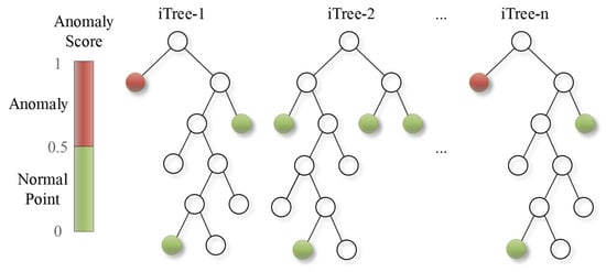
Figure 2. Schematic diagram of iForest anomaly detection principle and results.

2.2.2. Dynamic Threshold Isolation Forest

While the iForest algorithm has demonstrated satisfactory performance in previous outlier detection tasks, the standard iForest still exhibits certain limitations in practical applications, particularly in threshold selection. When detecting outliers, iForest typically employs a fixed threshold to determine whether a data point is anomalous. This setup leads to the following issues: (i) When the data distribution is uneven or the boundary between outliers and normal values is ambiguous, iForest may produce false positives or false negatives; (ii) A fixed threshold cannot adapt to dynamic changes in the data, resulting in poor model generalization; (iii) During the execution of the iForest algorithm, the calculation of anomaly scores relies on preset parameters, and a fixed threshold cannot correct subjective errors in parameter configuration, thereby leading to misjudgments. To address these limitations, this paper proposes a Dynamic Threshold Isolation Forest (DTIF) algorithm, which introduces the Otsu method to improve the threshold selection mechanism, thereby enhancing the accuracy and robustness of anomaly detection.

Otsu’s Method, originally proposed by Nobuyuki Otsu [32] in 1979, is a classical adaptive thresholding technique from image processing. This algorithm is based on the grayscale distribution characteristics of an image. By calculating the inter-class variance statistic under different segmentation thresholds, it selects the critical value that maximizes the difference between the foreground and background regions as the optimal segmentation threshold. The specific steps for threshold determination are as follows:

Step 1: For a given dataset or image, compute its grayscale histogram, representing the frequency of occurrence for each grayscale value.

Step 2: Normalize the histogram into a probability distribution, where the probability of each grayscale value is $p_i={\displaystyle \frac{n_i}{N}}$, with $n_i$ being the frequency of grayscale value $i$ and $N$ being the total number of pixels or samples.

Step 3: Iterate through all possible thresholds. For each candidate threshold $t$, divide the data into Class 1 (grayscale value $\le t$) and Class 2 (grayscale value $> t$).

Step 4: For each threshold $t$, compute the inter-class variance ${\sigma }_B^2\left(t\right)$ using the following formula:

$${\sigma }_B^2\left(t\right)={\mathit{w}}_0\left(t\right)·{\mathit{w}}_1\left(t\right)·{\left({\mathsf{\mu }}_0\left(t\right)-{\mathsf{\mu }}_1\left(t\right)\right)}^2$$

(11)

where ${\mathit{w}}_0\left(t\right)$ and ${\mathit{w}}_1\left(t\right)$ are the probability weights of Class 1 and Class 2, respectively, and ${\mathsf{\mu }}_0\left(t\right)$ and ${\mathsf{\mu }}_1\left(t\right)$ are the mean values of Class 1 and Class 2. Their calculation formulas are given by Equations (12) and (13):

$${\mathit{w}}_0\left(t\right)={\displaystyle \sum _{i=0}^t{p}_i}, {\mathit{w}}_1\left(t\right)={\displaystyle \sum _{i=t+1}^{L-1}{p}_i}$$

(12)

$${\mathsf{\mu }}_0\left(t\right)={\displaystyle \frac{{\displaystyle \sum _{i=0}^{t}i·p_i}}{{\mathit{w}}_0\left(t\right)}}, {\mathsf{\mu }}_1\left(t\right)={\displaystyle \frac{{\displaystyle \sum _{i=t+1}^{L-1}i·p_i}}{{\mathit{w}}_1\left(t\right)}}$$

(13)

where $L$ is the total number of grayscale levels. For example, in an 8-bit image, $L$= 256.

Step 5: Select the threshold $t^{*}$ that maximizes the inter-class variance ${\sigma }_B^2\left(t\right)$ as the optimal threshold:

$$t^{*}=\arg \underset{t}{\max }{\sigma }_B^2\left(t\right)$$

(14)

The DTIF algorithm proposed in this paper employs Otsu’s method to automatically determine the optimal threshold from the anomaly score histogram generated by iForest, thereby establishing a dynamic criterion for anomaly detection. The implementation steps of DTIF are as follows:

Step 1: iForest model training. The iForest model is applied to the preprocessed dataset to compute anomaly scores for all data points.

Step 2: Anomaly score histogram construction. The algorithm generates a histogram of the anomaly scores produced by iForest, recording both the frequency count (histogram height) and bin boundaries (histogram x-axis) for each interval. The central value of each bin serves as input for subsequent Otsu threshold calculation.

Step 3: Optimal threshold determination using Otsu’s method. The histogram frequencies are normalized to create a probability distribution by dividing each bin count by the total frequency. For each potential threshold (represented by bin centers), the algorithm calculates the inter-class variance between two groups: normal data points and anomalies. The threshold yielding maximum inter-class variance is selected as the optimal cutoff, achieving adaptive threshold adjustment for iForest’s anomaly scores.

The core algorithm flow of DTIF is as follows Algorithm 1:

Algorithm 1. The core algorithm flow of DTIF.

(1) Input: Time-series displacement monitoring data with timestamps and displacement values (2) Initialization Phase: Load dataset: Excel file containing ‘Monitoring Date (Y/M)’ and ‘Displacement (mm)’ Preprocess data: Convert timestamps to datetime format Extract feature vector: Displacement values as primary feature (3) Isolation Forest Training Phase: Initialize Isolation Forest model with parameters:   n_estimators = 100   contamination = ‘auto’   random_state = 42 Train model on displacement data Calculate anomaly scores using decision_function() (4) Dynamic Threshold Calculation Phase: Generate histogram of anomaly scores with 30 bins Apply Otsu’s method to find optimal threshold: For each possible threshold t in histogram bins:   Calculate class probabilities: w0, w1   Compute class means: μ0, μ1   Calculate between-class variance: σ2_B(t) = w0·w1·(μ0 − μ1)2 Select final_threshold t* that maximizes σ2_B(t) (5) Anomaly Detection Phase: Label anomalies: anomaly = −1 if anomaly_score < final_threshold, else 1 Extract detected anomalies based on dynamic threshold (6) Performance Evaluation Phase: Calculate evaluation metrics:   Accuracy (ACC) = (TP + TN)/total_samples   False Positive Rate (FPR) = FP/(FP + TN)   False Negative Rate (FNR) = FN/(FN + TP)   True Negative Rate (TNR) = TN/(TN + FP) Generate visualization plots for results analysis

3. Construction of RF Prediction Model Based on Feature Selection and Parameter Optimization

Dam displacement is influenced by multiple environmental factors in a complex manner, exhibiting highly nonlinear and uncertain variation patterns. Traditional statistical models and deterministic models often suffer from insufficient accuracy and poor generalization ability when dealing with complex displacement data. Random Forest (RF), as an ensemble learning algorithm, demonstrates significant advantages in dam displacement prediction due to its resistance to overfitting and strong capability in modeling nonlinear relationships. However, the performance of RF heavily relies on feature selection and hyperparameter optimization. Unreasonable feature inputs may lead to increased model complexity and reduced prediction accuracy, while unoptimized hyperparameters can limit the model’s performance. To address these challenges, this section proposes a method for constructing an RF prediction model based on feature selection and parameter optimization. First, the LASSO algorithm is employed to analyze and screen the importance of displacement feature factors, extracting an optimal feature subset. Subsequently, an Improved Reptile Search Algorithm (IRSA) is adopted to optimize the hyperparameters of the RF model, thereby enhancing its prediction accuracy and robustness.

3.1. Displacement Statistical Model and Feature Selection

3.1.1. Statistical Model

During dam displacement safety monitoring, various environmental variables exert continuous and multidimensional influences on the dam. To accurately analyze the mechanisms by which these variables affect dam displacement and achieve scientific prediction and evaluation of displacement, numerous statistical displacement models have been developed [33,34,35,36,37]. Among these, the Hydrostatic-Seasonal-Time (HST) model is the most widely used for dam displacement analysis and prediction [38]. As shown in Equation (15), the dam displacement $\delta$ in the HST model consists of three components:

$$\delta ={\delta }_H+{\delta }_T+{\delta }_{\theta }$$

(15)

where ${\delta }_H$, ${\delta }_T$, and ${\delta }_{\theta }$ represent the hydraulic pressure, temperature, and time-effect components, respectively.

(1)

Hydrostatic pressure component ${\delta }_H$

The hydrostatic pressure induces three main displacement components: (1) Sliding displacement (${\delta }_{1H}$) referring to horizontal sliding of the dam body; (2) Rotational displacement (${\delta }_{2H}$) caused by downstream tilting or foundation rotation, resulting from compression on the upstream face and tension on the downstream face; and (3) Flexural displacement (${\delta }_{3H}$) due to uneven force distribution along the dam height, manifesting as S-shaped bending with the crest displacing towards the reservoir and the base constrained by the foundation. These components are illustrated in Figure 3.

Figure 3. Three types of dam displacements caused by hydrostatic pressure. (a) Hydrostatic displacement. (b) Displacement from rock deformation. (c) Displacement from rock rotation.

In the HST model, the hydrostatic pressure component ${\delta }_H$ is typically modeled as a polynomial function of the water level:

$${\delta }_H={\displaystyle \sum _{i=1}^n\left(a_i{H}^i\right)}$$

(16)

where $H$ is the upstream water level; $a_i$ are the fitting parameters for the hydrostatic component determined by the least squares method; and $n$ is generally 4 for arch dams (or 3 for gravity dams).

(2)

Temperature component ${\delta }_T$

The temperature component ${\delta }_T$ primarily arises from temperature variations within the dam body and its foundation, which are closely related to external air temperature. For arch dams, after the complete dissipation of concrete hydration heat, the internal temperature distribution can be approximately considered steady-state. Based on this characteristic, the temperature component is typically calculated using a combination of harmonic sine and cosine functions, as shown in Equation (17). This approach effectively captures the periodic nature of temperature variations, thereby more accurately reflecting the dam’s response to seasonal climate conditions.

$${\delta }_T={\displaystyle \sum _{j=1}^2\left(b_{1j}\sin \frac{2\pi jt}{365}+b_{2j}\cos \frac{2\pi jt}{365}\right)}$$

(17)

where $b_{1j}$ and $b_{2j}$ are the fitting parameters for the temperature component, and $t$ is the cumulative number of days since the initial measurement date.

(3)

Time-effect component ${\delta }_{\theta }$

The time-effect component ${\delta }_{\theta }$ exhibits high complexity, with the creep behavior of concrete and rock being the dominant influencing factors. For concrete arch dams, the time-effect component initially shows rapid growth and then gradually stabilizes. The accumulated displacement variation resulting from this process can be modeled using a combination of logarithmic and linear functions:

$${\delta }_{\theta }=c_1\theta +c_2\ln \theta$$

(18)

where $c_1$ and $c_2$ are the fitting parameters for the time-effect component; and $\theta$ is the time-varying factor, defined as $\theta =t/100$. By combining Equations (15)–(18), the final statistical model for arch dam displacement is expressed as:

$$\delta =a_0+{\displaystyle \sum _{i=1}^4\left(a_i{H}^i\right)}+{\displaystyle \sum _{j=1}^2\left(b_{1j}\sin \frac{2\pi jt}{365}+b_{2j}\cos \frac{2\pi jt}{365}\right)}+c_1\theta +c_2\ln \theta +\epsilon$$

(19)

where $a_0$ is a constant accounting for the influence of the initial state; and $\epsilon$ represents the random residual.

Based on Equation (19), an initial feature factor set ${\mathit{X}}_0$ for the displacement prediction model can be obtained, which consists of the hydrostatic pressure factor set ${\mathit{X}}_H$, the temperature factor set ${\mathit{X}}_T$, and the time-effect factor set ${\mathit{X}}_{\theta }$:

$${\mathit{X}}_0=\left[{\mathit{X}}_H,{\mathit{X}}_T,{\mathit{X}}_{\theta }\right]=\left[H,H^2,H^3,H^4,\sin {\displaystyle \frac{2\pi t}{365}},\cos {\displaystyle \frac{2\pi t}{365}},\sin {\displaystyle \frac{4\pi t}{365}},\cos {\displaystyle \frac{4\pi t}{365}},\theta ,\ln \theta \right]$$

(20)

where

$${\mathit{X}}_H=\left[x_1,x_2,x_3,x_4\right]=\left[H,H^2,H^3,H^4\right]$$

(21)

$${\mathit{X}}_T=\left[x_5,x_6,x_7,x_8\right]=\left[\sin {\displaystyle \frac{2\pi t}{365}},\cos {\displaystyle \frac{2\pi t}{365}},\sin {\displaystyle \frac{4\pi t}{365}},\cos {\displaystyle \frac{4\pi t}{365}}\right]$$

(22)

$${\mathit{X}}_{\theta }=\left[x_9,x_{10}\right]=\left[\theta ,\ln \theta \right]$$

(23)

While HST-based synthetic features can exhibit multicollinearity, the employed LASSO algorithm inherently mitigates this issue through L1 regularization. The algorithm’s tendency to select a single representative from groups of correlated variables helps minimize statistical redundancy. Furthermore, the ensemble approach of Random Forest provides additional robustness against residual multicollinearity in the selected feature subset.

3.1.2. LASSO Algorithm

In general, not all factors in the initially constructed feature set contribute positively to the displacement prediction model. Some factors may be redundant or irrelevant, increasing the complexity of the model without improving its performance and potentially even causing significant interference in the prediction results. Therefore, selecting the optimal features from the initial feature set ${\mathit{X}}_0$ is a crucial step in building a high-accuracy prediction model. In this paper, the Least Absolute Shrinkage and Selection Operator (LASSO) algorithm is used to analyze and select the importance of displacement feature factors, thereby enhancing the model’s prediction accuracy and interpretability.

The LASSO algorithm [39] is a feature selection method based on L1 regularization. By introducing a penalty term to constrain the coefficients in the regression model, the coefficients of some unimportant variables are shrunk, achieving feature selection and model sparsification. The loss function of LASSO regression can be expressed as:

$$L_{Lasso}\left(\beta \right)={\displaystyle \sum _{i=1}^n{\left(y_i-{\beta }_0-{\displaystyle \sum _{j=1}^p{x}_{ij}{\beta }_j}\right)}^2}+\lambda {\displaystyle \sum _{j=1}^p\left|{\beta }_j\right|}$$

(24)

where the squared error term ${\displaystyle \sum _{i=1}^n{\left(y_i-{\beta }_0-{\displaystyle \sum _{j=1}^p{x}_{ij}{\beta }_j}\right)}^2}$ represents the loss function of ordinary least squares, used to measure the difference between the model’s predicted value ${\beta }_0-{\displaystyle \sum _{j=1}^p{x}_{ij}{\beta }_j}$ and the actual value $y_i$; ${\beta }_0$ is the intercept term (constant); ${\beta }_j$ is the regression coefficient of the j-th feature; $x_{ij}$ represents the j-th feature variable of the i-th sample; $\lambda {\displaystyle \sum _{j=1}^p\left|{\beta }_j\right|}$ is the L1 regularization term, and $\lambda$ is the regularization parameter, used to control the strength of the regularization term.

In dam displacement prediction, the LASSO algorithm can select the optimal feature subset by minimizing the objective function, providing high-quality feature input for the subsequent construction of the random forest model.

3.2. Random Forest Model

3.2.1. Principle of Random Forest

Random Forest (RF) is a machine learning algorithm based on ensemble learning [40], which improves model performance and robustness by constructing multiple decision trees and combining their prediction results. As shown in Figure 4, the core idea of RF lies in introducing randomness to generate diverse decision trees and integrating the prediction results of these trees through voting or averaging, thereby reducing the risk of overfitting of a single decision tree and enhancing the model’s generalization ability.

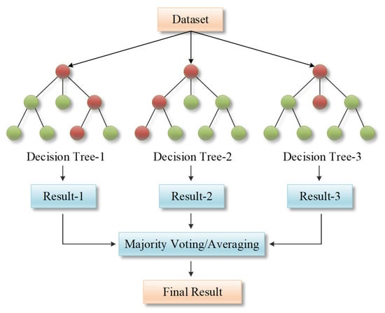
Figure 4. Workflow of the Random Forest algorithm.

The construction steps of RF are as follows:

Step 1: Data sampling. Randomly draw $n$ samples (with replacement) from the original dataset to generate a subset of data, each of which is used to train a decision tree. Due to the random sampling, the data used for each tree is slightly different, thus increasing the diversity of the model.

Step 2: Random feature selection. When constructing each decision tree, instead of using all features for branching, m features are randomly selected from all features. This random selection of features further increases the differences between trees and avoids all trees using the same features for branching.

Step 3: Constructing decision trees. Use the sampled data and randomly selected features to construct a complete decision tree. The construction of decision trees typically employs a recursive splitting method, selecting the best feature and split point to maximize the purity of the subsets (such as Gini index or information gain).

Step 4: Ensemble prediction. For classification tasks, the Random Forest integrates the prediction results of all decision trees through voting, selecting the category with the most votes as the final prediction. For regression tasks, the Random Forest obtains the final result by averaging the prediction values of all decision trees.

3.2.2. Hyperparameters of Random Forest

The performance and effectiveness of RF heavily rely on the settings of its hyperparameters, and properly choosing hyperparameters can significantly enhance the model’s prediction accuracy and generalization ability [41]. The numerous hyperparameters of RF can be roughly divided into three categories: hyperparameters related to the forest, hyperparameters related to the trees themselves, and splitting criteria. The splitting criteria are used to define the impurity measure when branching in decision trees. For classification tasks, the criterion is usually set as the Gini coefficient, while for regression tasks, it is typically set as Mean Squared Error (MSE) or Mean Absolute Error (MAE). For the dam displacement prediction, which is a regression problem, MSE is adopted as the splitting criterion. Among the other two categories of RF hyperparameters, the following five relatively important hyperparameters are selected in this paper for subsequent model optimization:

(1)

Ntree. Ntree refers to the number of decision trees in the RF. Increasing Ntree can improve the stability and accuracy of the model but also increases computational cost. The search space for Ntree is set to $\left[50,300\right]$ in this paper.

(2)

MaxDepth. MaxDepth refers to the maximum depth of a single decision tree, used to limit the growth of the tree and prevent overfitting. The search space for MaxDepth is set to $\left[1,20\right]$ in this paper.

(3)

MinSplit. MinSplit refers to the minimum number of samples required for a node to be split. Appropriately increasing this value can prevent the tree from becoming too complex and causing overfitting. The search space for MinSplit is set to $\left[2,10\right]$ in this paper.

(4)

MinLeaf. MinLeaf is the minimum number of samples required for a leaf node. Similarly, appropriately increasing this value can reduce the risk of overfitting. The search space for MinLeaf is set to $\left[1,5\right]$ in this paper.

(5)

MaxFeatures. MaxFeatures refers to the maximum number of features considered when branching in each decision tree, used to control the randomness of feature selection and increase feature diversity. The search space for MaxFeatures is set to $\left[1,N\right]$ in this paper, where $N$ is the total number of features in the training data.

3.3. Improved Reptile Search Algorithm

3.3.1. Principle of the Reptile Search Algorithm

The Reptile Search Algorithm (RSA) is a metaheuristic algorithm proposed by Abualigah et al. [29] in 2022, inspired by the hunting behavior of crocodiles. As shown in Figure 5, the algorithm draws inspiration from the unique two-phase hunting strategy of crocodiles.

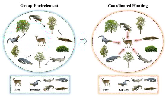
Figure 5. Diagram of the crocodile hunting mechanism in the RSA.

Although crocodiles often exhibit lazy and static behavior, they can explode with extreme attacking efficiency when hunting. Their group-coordinated foraging process demonstrates a dynamic balance between environmental exploration and resource exploitation. The RSA deconstructs crocodile predation behavior into two core strategies—environmental exploration (group encirclement) and resource exploitation (cooperative hunting), which are further refined into four progressive behavioral modes: expanding the search range through a high-stepping gait, crawling closer to the target in a low-profile manner, precise encircling through group collaboration, and team coordination during the prey capture phase. To align with the design concept of simplifying parameters in intelligent algorithms, RSA maps these four progressive behavioral modes into operational rules for different iteration stages in the optimization process. By simulating a single complete crocodile hunting process, RSA achieves dynamic regulation of global search and local exploitation, forming a unique optimization mechanism that combines environmental adaptability and convergence efficiency. The optimization process of RSA can be divided into the following steps:

Step 1: Initialization of candidate solutions. RSA first randomly generates a set of candidate solutions, each representing a potential solution in the search space. For the j-th feature dimension of the i-th candidate solution $x_{i,j}$, its initial value can be calculated using the following formula:

$$x_{i,j}=ran{d}_{\in U\left(0,1\right)}\times \left(U{B}_j-L{B}_j\right)+L{B}_j, i\in \left\{1,\dots ,N\right\} and i\in \left\{1,\dots ,M\right\}$$

(25)

where $U{B}_j$ and $L{B}_j$ represent the upper and lower bounds of the j-th feature dimension, respectively; $ran{d}_{\in U\left(0,1\right)}$ is a random number uniformly distributed within the range $\left[0,1\right]$; $N$ is the total number of candidate solutions; and $M$ is the number of feature dimensions.

Step 2: Encircling phase, which is the global exploration mechanism of the algorithm. The exploration phase of RSA simulates the encircling behavior of crocodiles before preying, mainly including high-walk ($t\le T/4$) and belly-walk ($T/4<t\le T/2$) movements. The update formula for candidate solutions is as follows:

$$x_{i,j}\left(t+1\right)=\left\{\begin{array}{l}-n_{i,j}\left(t\right)·\beta ·Bes{t}_j\left(t\right)-ran{d}_{\in \left[1,N\right]}·R_{i,j}\left(t\right), t\le {\displaystyle \frac{T}{4}}\\ ES\left(t\right)·Bes{t}_j\left(t\right)·x_{\left(ran{d}_{\in \left[1,N\right]},j\right)}, \hspace{1em} {\displaystyle \frac{T}{4}}<t\le {\displaystyle \frac{T}{2}}\end{array}\right.$$

(26)

where t is the current iteration number, $T$ is the set maximum number of iterations; $Bes{t}_j\left(t\right)$ is the current optimal solution for the j-th feature dimension; $n_{i,j}$ is the hunting operator for the j-th feature dimension of the i-th candidate solution; $\beta$ is a parameter that controls the exploration accuracy, typically set to 0.1; $R_{i,j}\left(t\right)$ is a reduction function used to narrow the search area; and $ES\left(t\right)$ is the evolutionary sensing probability ratio, which decreases from 2 to −2 as the iteration progresses.

Step 3: Hunting phase, which is the local exploitation mechanism of the algorithm. The collaborative hunting phase is triggered when the RSA is halfway through its iterations. This phase gradually narrows the encirclement through two hunting strategies: coordinated encircling ($T/2<t\le 3T/4$) and joint hunting ($t>3T/4$), ultimately achieving efficient capture of the prey. In these two strategies, candidate solutions are updated using the following formula:

$$x_{i,j}\left(t+1\right)=\left\{\begin{array}{l}ran{d}_{\in \left[-1,1\right]}·Bes{t}_j\left(t\right)·P_{i,j}\left(t\right), \hspace{1em}\hspace{1em}\hspace{1em} {\displaystyle \frac{T}{2}}<t\le {\displaystyle \frac{3T}{4}}\\ Bes{t}_j\left(t\right)-n_{i,j}\left(t\right)·\epsilon -ran{d}_{\in \left[-1,1\right]}·R_{i,j}\left(t\right), {\displaystyle \frac{3T}{4}}<t\le T\end{array}\right.$$

(27)

where $P_{i,j}$ is the percentage difference for the j-th feature dimension of the i-th candidate solution, calculated using Formula (28); $\epsilon$ is a small value.

$$P_{i,j}\left(t\right)=\alpha +{\displaystyle \frac{x_{i,j}-M\left(x_i\right)}{Bes{t}_j\left(t\right)·\left(U{B}_j-L{B}_j\right)+\epsilon }}$$

(28)

where $M\left(x_i\right)$ is the average position of the i-th candidate solution; and $\alpha$ is a sensitivity parameter that, along with $\beta$ in Equation (26), controls the exploration accuracy during iterations, typically set to a fixed value of 0.1.

Step 4: Evaluating fitness and outputting the optimal solution. In each iteration, the quality of candidate solutions is evaluated using a predefined fitness function. The algorithm stops when it reaches the maximum number of iterations or satisfies the convergence criteria, and selects the candidate solution with the minimum fitness value as the optimal solution.

3.3.2. Algorithm Improvement Strategies

Although RSA demonstrates certain advantages in solving complex optimization problems, it still has deficiencies in global search capability, convergence speed, and local exploitation accuracy [42]. To further enhance the performance, this paper introduces multiple improvements to the standard RSA by incorporating strategies such as chaotic mapping, dynamic parameter adjustment, and Lévy flight perturbation. By introducing these strategies, the algorithm not only better balances global search and local exploitation but also effectively avoids falling into local optima. The following are the improvement strategies and their implementation methods.

(1)

Tent chaotic mapping

The standard RSA typically uses random generation for population initialization, which may lead to insufficient population diversity and cause the algorithm to fall into local optima. This paper introduces Tent chaotic mapping to initialize the population, generating an initial population with good uniformity and randomness through chaotic mapping, thereby enhancing the algorithm’s global search capability. Tent chaotic mapping is a simple and efficient chaotic mapping method [43], which generates a chaotic sequence $Z_{i,j}$ with high randomness and ergodicity through its inherent chaotic characteristics:

$$Z_{i+1,j}=\left\{\begin{array}{l}{\displaystyle \frac{Z_{i,j}}{u}}, \hspace{1em}0\le Z_{i,j}\le u\\ {\displaystyle \frac{1-Z_{i,j}}{1-u}}, u<Z_{i,j}\le 1\end{array}\right.$$

(29)

where $u$ is used to maintain algorithm randomness and $u\subset rand\left(0,1\right)$. Combining the chaotic sequence $Z_{i,j}$ with Equation (25) further generates the initial position sequence $X_{i,j}$ of reptile individuals in RSA within the search area:

$$X_{i,j}=Z_{i,j}\times \left(U{B}_j-L{B}_j\right)+L{B}_j, i\in \left\{1,\dots ,N\right\} and i\in \left\{1,\dots ,M\right\}$$

(30)

(2)

Dynamic adjustment of control parameters

In the standard RSA, the control parameters $\alpha$ and $\beta$ in Equations (26) and (28) are usually fixed, which limits the algorithm’s adaptability to some extent. Therefore, this paper proposes a strategy for dynamically adjusting control parameters, adjusting them based on the current iteration number $t$ and the total number of iterations $T$ to balance the algorithm’s global search and local exploitation capabilities. The specific formula is as follows:

$$\alpha =0.3\times \left(1-{\displaystyle \frac{t}{T}}\right), \beta =0.1\times {\displaystyle \frac{t}{T}}$$

(31)

Through the adjustment in Equation (31), RSA will focus more on global search in the early iterations and more on local exploitation in the later iterations, thereby improving the algorithm’s convergence speed and accuracy.

(3)

Lévy flight strategy

Standard RSA primarily relies on local search during the trapping phase, which can easily lead to local optimum traps. By introducing the Lévy flight strategy, this paper enables some individuals to perform long-distance jumps during the trapping phase, thereby expanding the search scope and avoiding premature convergence. Lévy flight is a random walk strategy based on the Lévy distribution, which is a non-Gaussian distribution characterized by power-law decay, with a higher probability of generating long steps in its tail. This characteristic allows Lévy flights to frequently make long-distance jumps during the search process, effectively escaping local optimum areas and exploring broader search spaces [44]. The probability density function of Lévy distribution can be expressed as:

$$L\left(x\right)~{\left|x\right|}^{-1-\beta }, 0<\beta <2$$

(32)

where $\beta$ is a parameter of the Lévy distribution that controls the distribution characteristics of step lengths. In the process of generating Lévy flight step lengths, random variables $u$ and $v$ that follow a normal distribution need to be generated first:

$$u~N\left(0,{\sigma }_u^2\right), v~N\left(0,{\sigma }_v^2\right)$$

(33)

where ${\sigma }_u$ and ${\sigma }_v$ are standard deviations, calculated as:

$${\sigma }_u={\left({\displaystyle \frac{\Gamma \left(1+\beta \right)·\sin \left(\pi \beta /2\right)}{\Gamma \left(\left(1+\beta \right)/2\right)·\beta ·2^{\left(\beta -1\right)/2}}}\right)}^{1/\beta }, {\sigma }_v=1$$

(34)

where $\Gamma$ denotes the gamma function. From this, the step length of the Lévy flight can be calculated as:

$$LS=\alpha ·{\displaystyle \frac{u}{{\left|v\right|}^{1/\beta }}}$$

(35)

where $\alpha$ is a small constant used to prevent excessively large step lengths from reducing search efficiency.

By adding a Lévy flight disturbance term $LS$ to the individual position update results during the trapping phase of the RSA, the risk of RSA falling into local optimum traps is further reduced.

(4)

Elite Opposition-based Learning (EOBL)

Elite Opposition-based Learning (EOBL) is a strategy widely applied in optimization algorithms [45]. Its core lies in expanding the exploration scope of the search space by constructing symmetric solutions to the current optimal solution. Specifically, this method takes the elite individuals in the current population, i.e., the solutions with the highest fitness, as the basis to generate their opposite solutions at symmetric positions in the search space. By comparing the fitness values of the elite solutions and their opposite solutions, better solutions are selected as candidates for the next generation.

For a solution $x_{i,j}$ in the RSA solution space, the formula for calculating its opposite solution $x_{i,j}^{*}$ is:

$$x_{i,j}^{*}=U{B}_j+L{B}_j-x_{i,j}$$

(36)

Although generating opposite solutions for all individuals in the current population can expand the search scope, computational resources may be wasted on low-quality solutions. Therefore, EOBL introduces information from elite individuals based on opposite solutions, thereby more efficiently guiding the search process. From Equation (36), the formula for calculating the elite opposite solution $x_{E,j}^{*}$ is:

$$x_{E,j}^{*}=U{B}_j+L{B}_j-x_{E,j}$$

(37)

where $x_{E,j}$ is the component of the elite individual in the j-th feature dimension.

During the hunting phase, standard RSA primarily relies on the current optimal solution for local exploitation, which may lead to inefficient search. By introducing EOBL in this paper, new candidate solutions are generated through opposition-based learning of the current optimal solution in RSA, further exploring high-quality solutions and accelerating the convergence speed of the algorithm.

3.3.3. Steps of the IRSA

Based on the principles of the standard RSA and incorporating the three improvement strategies discussed above, the IRSA is constructed with the following specific steps:

Step 1: Parameter Initialization. Set the basic parameters of the IRSA, including population size $N$, feature dimension $M$, maximum number of iterations $T$, define the Lévy flight parameter $\beta =1.5$, and set the proportion $p=0.1$ of individuals for elite opposition-based learning.

Step 2: Initial Population Generation Based on Tent Chaotic Mapping. Utilize Tent chaotic mapping according to Equations (29) and (30) to generate a chaotic sequence $Z_{i,j}$, and convert this chaotic sequence into initial solutions $X_{i,j}$ within the search space through uniform mapping, ensuring high diversity and uniform distribution of the population within the solution space.

Step 3: Calculate Initial Fitness and Optimal Solution. Evaluate the fitness values of all individuals in the initial population, and record the position $X_{best}$ of the current optimal individual and its corresponding fitness value.

Step 4: Dynamic Parameter Adjustment. Based on the current iteration number $t$, dynamically update the global search parameter $\alpha \left(t\right)$ and local exploitation parameter $\beta \left(t\right)$ through a linearly decreasing Equation (31), enabling the algorithm to focus more on global exploration in the early stages and local exploitation in the later stages.

Step 5: Position Update in the Trapping Phase. When $t\le T/2$, perform the position update in the trapping phase of the standard RSA for each individual according to the high-altitude stepping and abdominal walking strategies in Equation (26), generating a preliminary position $X_i^{\prime }$.

Step 6: Lévy Flight Perturbation. Introduce the Lévy flight strategy according to Equations (33)–(35) to apply random perturbations to the updated positions, generating new positions $X_i^{″}$ with Lévy step lengths, and perform boundary truncation for any out-of-bounds values.

Step 7: Position Update in the Hunting Phase. When $t>T/2$, update individual positions based on the coordinated trapping and joint hunting strategies in Equation (27), guiding the population to converge towards high-potential regions based on the current optimal solution $X_{best}$.

Step 8: Elite Opposition-based Learning Optimization. Select the top $p\times N$ elite individuals in terms of fitness from the population, generate their opposite solutions based on Equation (37), and retain the better individuals by comparing the fitness of elite solutions and their opposite solutions to enhance the population quality.

Step 9: Update Global Optimal Solution and Termination Criteria. Compare the fitness values of all individuals in the current population, update the global optimal solution $G_{best}$. Terminate the algorithm and output the optimal solution if the maximum number of iterations $T$ is reached or the convergence threshold condition is met; otherwise, return to Step 4 for continued iteration. Specifically, if the fitness improvement stagnates (with a relative change of <0.01% over five consecutive iterations), the solution is accepted as optimal, regardless of whether the maximum iterations are reached. This dual criteria ensure that the algorithm does not terminate prematurely without achieving a stable solution.

The core algorithm flow of IRSA is shown in Algorithm 2.

Algorithm 2. The core algorithm flow of IRSA.

(1) Input Parameters: Population size (N), Maximum iterations (T), Lower and upper bounds (LB, UB) Problem dimension (Dim), Training data (X_data, y_data) (2) Initialization Phase: 1. Initialize population using Tent chaotic mapping:    X = Tent_Chaos(N, Dim)    Scale positions to search space: X = LB + (UB − LB) × X 2. Initialize best solution: Best_P = X[0], Best_F = ∞ (3) Main Optimization Loop (for t = 1 to T): 1. Dynamic Parameter Adjustment:    α = 0.3 × (1 − t/T) // Global exploration parameter    β = 0.1 × (t/T)    // Local exploitation parameter    ES = random value in [−1, 1]   // Exploration factor 2. Fitness Evaluation:    For each individual i in population:        current_fitness = Objective_Function(X[i], X_data, y_data)        Update Best_P and Best_F if improved 3. Encircling Phase (Global Exploration when t < T/2):    For each individual i:        Calculate hunting operator: R = (Best_P − X[i])/(Best_P + ε)        Compute percentage difference: P = α + (X[i] − mean(X))/(Best_P × (UB − LB) + ε)        Apply movement strategies:        -With 50% probability: Apply Lévy flight perturbation            X[i] = Best_P − Eta × β − R × rand() + Levy_Flight(Dim)        -Otherwise: Use exploratory movement            X[i] = Best_P × X[random] × ES × rand() 4. Hunting Phase (Local Exploitation when t ≥ T/2):    For each individual i:        -Apply Elite Opposition-Based Learning:            opposite_solution = LB + UB − Best_P            Evaluate opposite solution fitness            Update best solution if improved        -Local refinement:            X[i] = Best_P × (1 + Gaussian_noise × 0.1) 5. Boundary Constraint Handling:    X = clip(X, LB, UB) // Ensure solutions remain within bounds (4) Objective Function Definition: Function Objective_Function(params, X_data, y_data):   Initialize Random Forest classifier with hyperparameters:            n_estimators = int(params [0])            max_depth = int(params [1])            min_samples_split = int(params [2])            min_samples_leaf = int(params [3])            max_features = int(params [4])    Perform 5-fold cross-validation    Return negative mean accuracy (for minimization) (5) Output: Best hyperparameters (Best_P), Best accuracy (−Best_F), Convergence history (Conv)

3.3.4. Performance Testing Experiment and Analysis for IRSA

To validate the global optimization capability of the IRSA, this study constructs an algorithm performance evaluation framework based on the characteristics of multimodal function spaces. Four benchmark functions with typical topological features, namely Sphere, Rastrigin, Ackley, and Rosenbrock, are selected. By comparing the convergence speed and solution accuracy indicators before and after the improvement, a quantitative analysis of the algorithm’s adaptability in nonlinear optimization scenarios is conducted. The experimental validation criterion is the success rate of detecting the global minimum of the functions, while the decay rate of iteration count is also recorded to quantify the efficiency gains of the algorithm. The mathematical forms and other basic properties of each test function are detailed in Table 1.

Table 1. Basic properties of four test functions.

Function	Number of Extrema	Expression	x-Range	Optimal Value
Sphere	Few	$f_1\left(x\right)={\displaystyle \sum _{i=1}^n{x}_i^2}$	[−5.12, 5.12]	$f_1\left(\overrightarrow{0}\right)=0$
Rastrigin	Many	$f_2\left(x\right)=10n+{\displaystyle \sum _{i=1}^n\left[x_i^2-10\cos \left(2\pi x_i\right)\right]}$	[−5.12, 5.12]	$f_2\left(\overrightarrow{0}\right)=0$
Ackley	Relatively many	$\begin{array}{l}{f}_3\left(x\right)=-20\exp \left(-0.2\sqrt{{\displaystyle \frac{1}{n}}{\displaystyle \sum _{i=1}^n{x}_i^2}}\right)\\ -\exp \left({\displaystyle \frac{1}{n}}{\displaystyle \sum _{i=1}^n\cos \left(2\pi x_i\right)}\right)+20+e\end{array}$	[−32.768, 32.768]	$f_3\left(\overrightarrow{0}\right)=0$
Rosenbrock	Few	$f_4\left(x\right)={\displaystyle \sum _{i=1}^{n-1}\left[100{\left(x_{i+1}-x_i^2\right)}^2+{\left(1-x_i\right)}^2\right]}$	[−2.048, 2.048]	$f_4\left(\overrightarrow{0}\right)=0$

To intuitively analyze the mathematical properties of the test functions, Figure 6 employs a three-dimensional visualization method to showcase the spatial topology of the benchmark functions. The surface morphology allows for clear identification of the functions’ nonlinearity intensity, multimodal characteristics (such as local extrema density), and optimal solution distribution patterns. In the design of the optimization experiments, the function output value $f\left(x\right)$ is defined as the basis for evaluating the population’s fitness, while the two-dimensional coordinates $\left(x,y\right)$ represent the position vector of an individual in the solution space. The global minimum search is conducted within the defined domain through the IRSA.

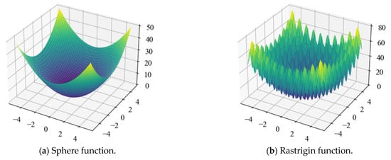
Figure 6. Three-dimensional plots of four benchmark functions.

The initial parameters of the algorithm include population size N, maximum number of iterations T, and dimension M. The experimental results are shown in Figure 7. From the comparison of convergence curves, it is evident that the improved RSA demonstrates significant advantages across all four types of test functions. In the Sphere unimodal function, IRSA achieves a precision of 10⁻¹³⁵ within just 5 iterations, representing an acceleration of approximately 10 times compared to RSA, which validates the effectiveness of Tent chaotic initialization in guiding the search direction. When confronted with the Rastrigin multimodal function, IRSA successfully escapes local optima traps through Lévy flight perturbations, also exhibiting a convergence speed about 10 times faster than RSA, thus proving its enhanced global exploration capability. In the Ackley non-convex function, the dynamic parameter adjustment mechanism of the improved algorithm ensures a steady descent of the convergence curve, avoiding the stage-wise stagnation observed in the baseline algorithm. For the Rosenbrock valley-shaped function, the EOBL strategy enables the improved algorithm to perform efficient fine-tuning searches in the later stages, achieving a precision improvement of over 10 times compared to the baseline algorithm. These results systematically indicate that the IRSA achieves an optimized reconstruction of the exploration-exploitation balance and demonstrates stronger robustness and universality, especially when dealing with high-dimensional and complex optimization problems.

Figure 7. Comparison of convergence performance between the original and improved RSA on benchmark test functions.

3.4. Establishment of a Dam Displacement Prediction Model

Combining the methods mentioned in Section 2 and Section 3, this paper constructs a two-stage dam displacement monitoring model, the DE-IRSA-RF model, which includes data cleaning and displacement prediction. Figure 8 illustrates the entire workflow of the DE-IRSA-RF model for displacement monitoring.

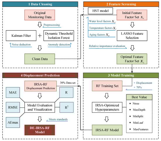
Figure 8. Schematic diagram of the DE-IRSA-RF model construction.

The specific steps for displacement prediction using the DE-IRSA-RF model are as follows:

Step 1: Determine the time series data for dam monitoring. In this paper, the first 70% of the monitoring data is selected as the training set, and the remaining 30% as the test set.

Step 2: Data cleaning. For the selected displacement time series data, KF is first applied for noise reduction, followed by the DTIF to detect and remove outliers.

Step 3: Determine the model inputs and output. Based on the HST model and Equations (20)–(23), the hydrostatic pressure factor ${\mathit{X}}_H$, the temperature factor ${\mathit{X}}_T$, and the time-effect factor ${\mathit{X}}_{\theta }$ are identified as the input variables for the model. The horizontal displacement of the dam is taken as the model’s output. The mathematical expression is:

$$\begin{array}{l} \delta =f\left(x_1,x_2,x_3,x_4,x_5,x_6,x_7,x_8,x_9,x_{10}\right)\\ =f\left(H,H^2,H^3,H^4,\sin {\displaystyle \frac{2\pi t}{365}},\cos {\displaystyle \frac{2\pi t}{365}},\sin {\displaystyle \frac{4\pi t}{365}},\cos {\displaystyle \frac{4\pi t}{365}},\theta ,ln\theta \right)\end{array}$$

(38)

Step 4: Select the final input factors. The LASSO algorithm is used to shrink the coefficients of the 10 displacement influencing factors from Step 3, and a comparison and validation of their relative importance are conducted. The factors that contribute most to displacement prediction are selected as the final inputs for the model.

Step 5: Data normalization. Each feature $x_i$ is normalized to the range $\left[0,1\right]$. The normalized value $x_i^{\prime }$ is calculated as follows:

$$x_i^{\prime }={\displaystyle \frac{x_i-\min \left(X\right)}{\max \left(X\right)-\min \left(X\right)}}$$

(39)

Step 6: Model training. On the training set data, IRSA is used to search for the optimal combination of hyperparameters for the RF model. The MSE is used for evaluation and validation, ultimately establishing the IRSA-RF prediction model.

Step 7: Model validation. The model is validated on the test set data. After reverse normalization of the output results, the displacement prediction accuracy is assessed based on the model performance evaluation metrics: Mean Absolute Error (MAE), Root Mean Squared Error (RMSE), Maximum Absolute Error (AE_max), Correlation Coefficient (R), and Coefficient of Determination (R²). The calculation formulas are as follows:

$$\mathrm{MAE}={\displaystyle \frac{1}{n}}{\displaystyle \sum _{i=1}^n\left|y_i-{\widehat{y}}_i\right|}$$

(40)

$$\mathrm{RMSE}=\sqrt{{\displaystyle \frac{1}{n}}{\displaystyle \sum _{i=1}^n{\left(y_i-{\widehat{y}}_i\right)}^2}}$$

(41)

$$\mathrm{A}{\mathrm{E}}_{\max }=\underset{i=1}{\overset{n}{\max }}\left|y_i-{\widehat{y}}_i\right|$$

(42)

$$\mathrm{R}={\displaystyle \frac{{\displaystyle \sum _{i=1}^n\left(y_i-\overline{y}\right)\left({\widehat{y}}_i-\overline{\widehat{y}}\right)}}{\sqrt{{\displaystyle \sum _{i=1}^n{\left(y_i-\overline{y}\right)}^2}}·\sqrt{{\displaystyle \sum _{i=1}^n{\left({\widehat{y}}_i-\overline{\widehat{y}}\right)}^2}}}}$$

(43)

$${\mathrm{R}}^2=1-{\displaystyle \frac{{\displaystyle \sum _{i=1}^n{\left(y_i-{\widehat{y}}_i\right)}^2}}{{\displaystyle \sum _{i=1}^n{\left(y_i-\overline{y}\right)}^2}}}$$

(44)

where $n$ is the total number of samples; $y_i$ is the true value of the i-th sample; ${\widehat{y}}_i$ is the predicted value of the i-th sample; $\overline{y}$ is the mean of the true values; and $\overline{\widehat{y}}$ is the mean of the predicted values. Smaller values of MAE, RMSE, and AEmax indicate better model prediction results. The value of R ranges from $\left[-1,1\right]$, with values closer to 1 or −1 indicating a stronger linear relationship between the predicted and true values. The value of R² ranges from $\left[0,1\right]$, with values closer to 1 indicating a stronger explanatory power of the model for the data.

3.5. Computational Environment and Implementation Details

This section provides a comprehensive description of the computational environment and the specific parameter configurations used for all algorithms discussed in this study.

The hardware and software configurations that formed the basis for all experiments are summarized in Table 2. This setup provided a stable and consistent platform for model training and evaluation.

Table 2. Computational Environment and Software Configuration.

Category	Component	Specification/Version
Hardware Environment	Processor (CPU)	AMD Ryzen 7 5800H
	Memory (RAM)	16 GB
	Operating System	Windows 11
Software Environment	Programming Language	Python 3.9.20
	Core Libraries	scikit-learn 1.5.1
		numpy 1.26.4
		pandas 2.2.2
		scipy 1.13.1
		PyTorch 2.5.1
	Visualization Library	matplotlib 3.9.2

The key hyperparameters and algorithmic settings for the proposed DTIF, IRSA models, and the baseline models (RF, LASSO, LSTM) are detailed in Table 3. These parameters were either determined through preliminary experiments or set to established default values common in the literature to ensure a fair comparison.

Table 3. Algorithm Parameters and Configuration.

Algorithm/Component	Parameter	Value/Setting
DTIF	n_estimators	100
	contamination	‘auto’
	random_state	42
	bins	30
IRSA	Population_size	30
	Max_iterations	100
	Dim	5
	Tent_u	0.7
	Lévy_β	1.5
RF—Search Space	n_estimators	[50, 300]
	max_depth	[1, 20]
	min_samples_split_range	[2, 10]
	min_samples_leaf_range	[1, 5]
	max_features_range	[1, N]
LASSO Regression	Model	LassoCV(cv = 10)
	eps	0.001
	n_alphas	100
	tol	0.0001
	max_iter	1000
	Scaling	StandardScaler
LSTM Model	LSTM Layer	1 layer, 50 units
	Output Layer	Dense (1)
	Optimizer	Adam
	Learning Rate	0.001
	Batch Size	32
	Epochs	50
	Loss Function	MSE

4. Engineering Case Application

4.1. Engineering Background

This paper validates and analyzes the effectiveness of the proposed displacement prediction framework using real monitoring data from a concrete double-curvature arch dam. The dam crest has an elevation of 391.6 m, with a maximum dam height of 49.6 m and a crest axis length of 149.7 m. The non-overflow dam crest on both banks is 4.0 m wide, with a base width of 8.8 m and a thickness-to-height ratio of 0.19. The catchment area above the dam site is 4148 km³, with an annual average discharge of 90.9 m³/s. The normal storage level is 380.00 m, corresponding to a storage capacity of 2.95 million m³, with a total storage capacity of 8.96 million m³ and an installed capacity of 2 × 15 MW. This project is a hydropower and water conservancy project primarily focused on power generation, with additional benefits such as tourism. Figure 9 provides an overall view of the dam.

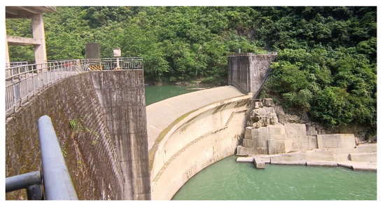
Figure 9. Overall view of the dam.

4.2. Dam Monitoring Data

The automated monitoring system for the arch dam obtained initial measurements on 25 December 2020. Daily observations of the dam’s horizontal displacement are primarily conducted through four inverted pendulum boreholes, labeled as DC1, DC2, DC4, and DC5. Specifically, DC1 and DC5 are located on the left and right dam abutments at the crest, respectively, while DC2 and DC4 are positioned at the left and right 1/4 dam sections, i.e., at the left and right side piers of the spillway crown. The downstream elevation view of the dam and the distribution of horizontal displacement monitoring points are shown in Figure 10.

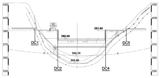
Figure 10. Layout of horizontal displacement monitoring points on the dam. The dashed line represents the original ground surface, the solid line indicates the excavation line, the solid line with three ‘x’ marks denotes the bottom of the highly weathered rock, and the solid line with two ‘x’ marks signifies the bottom of the slightly weathered rock.

This study focuses on the data from monitoring point DC2, which exhibits the maximum monitored physical quantity in terms of horizontal displacement. The monitoring data from points DC4 and DC5 will be used to test the generalization capability of the proposed model. Considering the completeness and periodic variation characteristics of displacement, water level, and temperature data, the selected data span should be no less than one year. The automated monitoring system recorded data at a daily frequency. Therefore, a total of 594 periods of automated observation data from the arch dam, collected between 13 January 2021, and 29 August 2022, are analyzed. The first 70% of the data is used as the training set, with the remaining data serving as the test set. During the monitoring period, the independent relative changes in the dam body’s horizontal displacement, upstream water level, and local temperature recorded at monitoring point DC2 are illustrated in Figure 11.

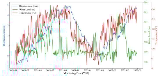
Figure 11. Relative independent changes in horizontal displacement, water level, and temperature at monitoring Point DC2.

4.3. Evaluation of Data Cleaning Effectiveness

4.3.1. Assessment of Kalman Filter’s Noise Reduction Performance

The horizontal displacement data from monitoring point DC2 was selected, and both KF and Particle Filter (PF), which is representative for handling nonlinear systems, were applied for noise reduction. In this comparative analysis, the original monitoring data served as the reference for MSE calculation under the premise that the KF and PF primarily target high-frequency noise reduction while preserving the underlying trend.

The results of the displacement monitoring data noise reduction are shown in Figure 12. To more intuitively compare the denoised displacement lines with the original, the process line after KF denoising is shifted up by 0.4 mm, while the corresponding PF process line is shifted down by 0.4 mm. It can be seen that the displacement data curves processed by both KF and PF are smoother compared to the original curve. To comprehensively evaluate the effectiveness of data noise reduction, the maximum (Max), minimum (Min), mean (Mean), median (Median), standard deviation (Std), signal-to-noise ratio (SNR), as well as the mean squared error (MSE) and correlation coefficient (R) between the filtered data and the true data, were calculated to quantitatively assess the performance of the noise reduction methods in dam displacement data denoising. Table 4 presents a comparison of the two methods across various indicators.

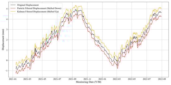
Figure 12. Comparison of displacement time series plots after KF and PF denoising.

Table 4. Statistical indicators before and after denoising of original displacement data.

Statistical Indicators	Original Displacement Data	KF Denoised Data	PF Denoised Data
Max (mm)	4.9700	4.9421	4.9263
Min (mm)	−0.9400	−0.9546	−0.8926
Mean (mm)	2.1106	2.1106	2.1051
Median (mm)	1.9850	1.9894	1.9529
Std (mm)	1.6753	1.6774	1.6749
MSE (mm2)	/	0.0015	0.0033
SNR (dB)	/	32.5978	29.4041
R	/	0.9997	0.9994

Table 4 shows that the Max, Min, Mean, and Median values after KF denoising are closer to the original data than those after PF, indicating that KF better preserves the data’s dynamic range and central tendency during the denoising process. The standard deviation after KF denoising slightly increases from 1.6753 mm to 1.6774 mm, suggesting that while reducing noise, KF may also slightly increase data dispersion. In terms of other indicators, the MSE after KF denoising is very small (0.0015 mm²), which is 37.50% lower than that of the PF method. The SNR after KF denoising reaches 32.5978 dB, an improvement of 5.16% compared to the PF method, indicating that noise is significantly suppressed and the signal quality is very high. The correlation coefficient R after KF denoising still performs better, with a value very close to 1 (0.9997), indicating a strong linear relationship between the denoised data and the original data. This further confirms that KF effectively removes noise while preserving the original trend of the data. Therefore, the KF method will be used in this paper for denoising horizontal displacement data.

4.3.2. Dynamic Threshold Isolation Forest for Outlier Detection

To systematically evaluate the performance of the proposed Dynamic Threshold Isolation Forest (DTIF) algorithm in identifying true outliers within dam safety monitoring datasets, this study simulates realistic dam deformation patterns by introducing anomalies based on two critical dimensions: outlier quantity and spatial arrangement. The injected anomalies emulate practical scenarios observed in dam monitoring, including sudden settlement due to foundation adjustment, measurement spikes from sensor faults, or transient shifts from rapid reservoir level changes. By combining outlier ratios (1%, 2%, 4%) and distribution patterns (isolated, consecutive, mixed), a test set with nine distinct outlier scenarios was constructed, as shown in Table 5. Outliers were generated within the range of $\left[\mu -4\sigma , \mu -3\sigma \right]\cup \left[\mu +3\sigma , \mu +4\sigma \right]$, where $\mu$ represents the mean and $\sigma$ denotes the standard deviation of the displacement data. This design ensures that both the magnitudes and durations (isolated or consecutive) of the anomalies reflect practical outlier patterns, thereby maintaining ecological validity for rigorously testing the DTIF algorithm under conditions that closely mirror real-world dam monitoring challenges.

Table 5. Outlier injection methods and groupings.

Anomaly Rate	Isolated 1	Consecutive 2	Mixed 3
1%	A1	A2	A3
2%	A4	A5	A6
4%	A7	A8	A9

¹ Each outlier exists as a single point; ² Each outlier appears as 2–3 consecutive data points; ³ Outliers coexist in both isolated and consecutive forms.

Performance metrics for outlier detection include accuracy (ACC), false positive rate (FPR), false negative rate (FNR), and specificity (TNR), corresponding to Equations (45)–(48). ACC measures the proportion of correctly classified samples, reflecting overall model performance. FPR indicates the rate of normal samples misclassified as outliers, while FNR quantifies missed detections of true outliers. TNR represents the proportion of correctly identified normal samples. Higher ACC/TNR and lower FPR/FNR values indicate superior outlier detection performance.

$$\mathrm{ACC}={\displaystyle \frac{TP+TN}{TP+TN+FP+FN}}$$

(45)

$$\mathrm{FPR}={\displaystyle \frac{FP}{TN+FP}}$$

(46)

$$\mathrm{FNR}={\displaystyle \frac{FN}{TP+FN}}$$

(47)

$$\mathrm{TNR}={\displaystyle \frac{TN}{TN+FP}}$$

(48)

where TP (True Positive) refers to the number of samples in which anomalies are correctly identified as anomalies; FP (False Positive) denotes the number of samples in which normal values are misclassified as anomalies; TN (True Negative) represents the number of samples in which normal values are correctly identified as normal; FN (False Negative) indicates the number of samples in which anomalies are erroneously identified as normal.

To avoid redundancy, representative results for each outlier ratio are presented. Figure 13, Figure 14 and Figure 15 illustrate detection outcomes for three classic methods, standard iForest, and DTIF on datasets A1 (1% isolated), A5 (2% consecutive), and A9 (4% mixed), respectively.

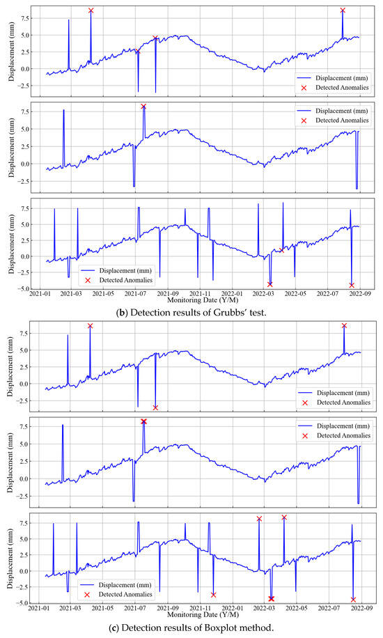
Figure 13. Detection results of three classical methods on datasets A1, A5, and A9.

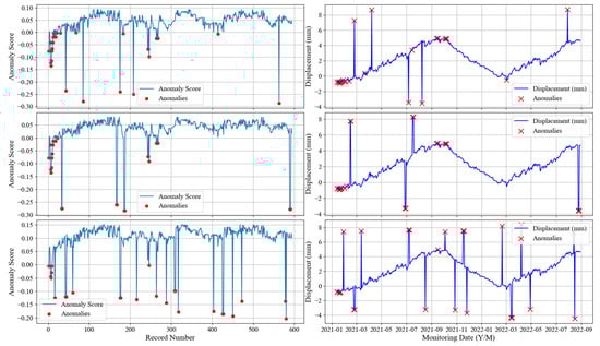
Figure 14. iForest detection results on datasets A1, A5, and A9.

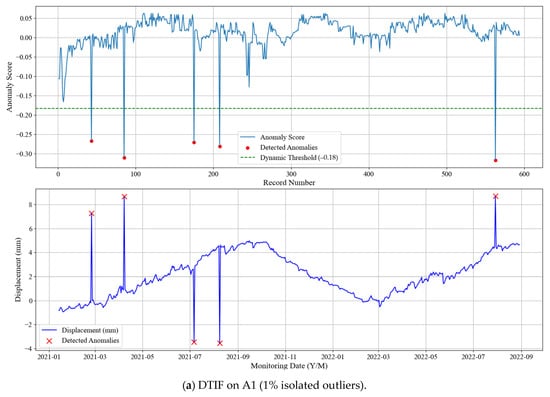
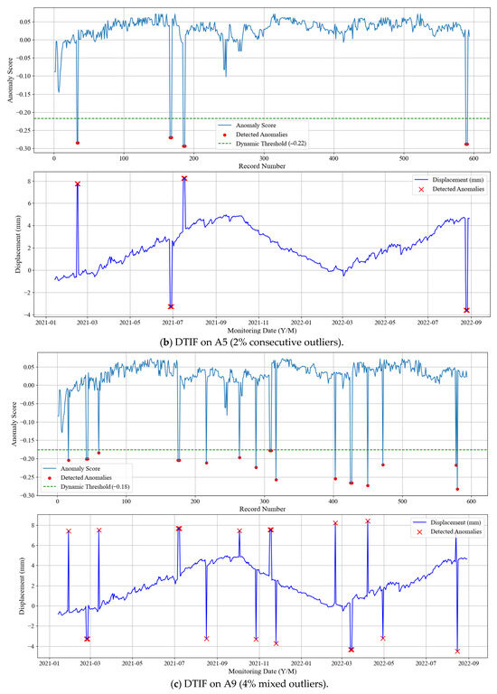
Figure 15. Outlier detection results of DTIF.

Figure 13 and Figure 14 reveal that the three classical methods exhibit frequent missed detections across all outlier ratios, while iForest produces excessive false alarms. In contrast, DTIF (Figure 15) achieves perfect detection (zero missed outliers or false alarms) in all scenarios. The dynamic threshold subplot demonstrates DTIF’s adaptive adjustment of anomaly scores, significantly reducing false positives compared to iForest’s fixed zero threshold. Table 6 compares the performance of the aforementioned methods under nine anomaly scenarios using four evaluation metrics: ACC, FPR, FNR, and TNR.

Table 6. The outlier detection performance metrics of different methods under nine conditions.

Data Set	Methods	ACC	FPR	FNR	TNR
A1	3σ criterion	0.9983	0.0000	0.2000	1.0000
	Grubbs’ test	0.9916	0.0034	0.6000	0.9966
	Boxplot	0.9966	0.0000	0.4000	1.0000
	iForest	0.9579	0.0424	0.0000	0.9576
	DTIF	1.0000	0.0000	0.0000	1.0000
A2	3σ criterion	1.0000	0.0000	0.0000	1.0000
	Grubbs’ test	0.9949	0.0000	0.6000	1.0000
	Boxplot	0.9966	0.0000	0.4000	1.0000
	iForest	0.9596	0.0407	0.0000	0.9593
	DTIF	1.0000	0.0000	0.0000	1.0000
A3	3σ criterion	0.9983	0.0000	0.2000	1.0000
	Grubbs’ test	0.9949	0.0000	0.6000	1.0000
	Boxplot	0.9983	0.0000	0.2000	1.0000
	iForest	0.9630	0.0374	0.0000	0.9626
	DTIF	1.0000	0.0000	0.0000	1.0000
A4	3σ criterion	0.9949	0.0000	0.2727	1.0000
	Grubbs’ test	0.9747	0.0103	0.8182	0.9897
	Boxplot	0.9933	0.0000	0.3636	1.0000
	iForest	0.9697	0.0309	0.0000	0.9691
	DTIF	1.0000	0.0000	0.0000	1.0000
A5	3σ criterion	0.9949	0.0000	0.2727	1.0000
	Grubbs’ test	0.9832	0.0000	0.9091	1.0000
	Boxplot	0.9865	0.0000	0.7273	1.0000
	iForest	0.9680	0.0326	0.0000	0.9674
	DTIF	1.0000	0.0000	0.0000	1.0000
A6	3σ criterion	0.9933	0.0000	0.3636	1.0000
	Grubbs’ test	0.9832	0.0051	0.6364	0.9949
	Boxplot	0.9933	0.0000	0.3636	1.0000
	iForest	0.9680	0.0326	0.0000	0.9674
	DTIF	1.0000	0.0000	0.0000	1.0000
A7	3σ criterion	0.9798	0.0000	0.5455	1.0000
	Grubbs’ test	0.9545	0.0140	0.8636	0.9860
	Boxplot	0.9781	0.0017	0.5455	0.9983
	iForest	0.9899	0.0105	0.0000	0.9895
	DTIF	0.9983	0.0017	0.0000	0.9983
A8	3σ criterion	0.9848	0.0000	0.3913	1.0000
	Grubbs’ test	0.9613	0.0000	1.0000	1.0000
	Boxplot	0.9848	0.0000	0.3913	1.0000
	iForest	0.9882	0.0123	0.0000	0.9877
	DTIF	1.0000	0.0000	0.0000	1.0000
A9	3σ criterion	0.9714	0.0000	0.7391	1.0000
	Grubbs’ test	0.9630	0.0018	0.9130	0.9982
	Boxplot	0.9731	0.0000	0.6957	1.0000
	iForest	0.9882	0.0123	0.0000	0.9877
	DTIF	1.0000	0.0000	0.0000	1.0000

The metrics in Table 6 clearly demonstrate that traditional outlier detection methods including the 3σ criterion, Grubbs’ test and boxplot method exhibit significant limitations. Without prior knowledge of data distribution, these three classical methods show substantial false negative problems. The 3σ criterion achieves an FNR of 20% in Scenario A1 (1% isolated outliers), with the FNR increasing to 27.27% in Scenario A4 (2% isolated outliers). Grubbs’ test fails completely to detect any outliers in Scenario A8 (4% consecutive outliers), indicating its poor sensitivity to sequential anomalies. In comparison with the standard iForest algorithm, DTIF shows significantly better outlier detection performance. Except for Scenario A7, DTIF achieves perfect scores across all evaluation metrics, successfully isolating all outliers from the data. Although iForest can detect all anomalies (FNR = 0), this comes at the cost of misclassifying normal data points, requiring manual secondary screening in practical engineering applications and resulting in low efficiency. Through algorithmic improvements, DTIF significantly reduces both FPR and FNR while maintaining high ACC and TNR, demonstrating greater robustness and reliability in outlier detection. The dynamic threshold strategy based on Otsu’s method proposed in this study provides notable enhancement to iForest’s outlier discrimination capability, significantly reducing misjudgment risks without requiring manual parameter tuning, and can be directly applied to complex anomaly scenarios such as dam displacement monitoring.

4.4. Optimal Feature Subset Selection

In the construction of a dam deformation prediction model, the selection of input factors has a decisive impact on model performance. To ensure the model accurately captures the key characteristics of dam deformation, two core issues must be addressed: (i) reducing multicollinearity among feature factors to avoid redundant information interfering with model learning, and (ii) ensuring the selected factors contain sufficient effective information to provide high-quality input data for the model. Therefore, optimizing the strategy for selecting input factors becomes a crucial step in improving the accuracy of dam deformation prediction models.

Following the LASSO-based deformation feature screening method proposed in Section 3.1, the optimal feature subset for the prediction model can be determined based on the LASSO correlation coefficients of the factors. Prior to LASSO regression, all HST-based feature factors were standardized using zero-mean, unit-variance normalization (StandardScaler) to ensure comparability of coefficients. Table 7 presents the LASSO correlation coefficients of each factor calculated from the monitoring data of the DC2 measuring point, which has the largest horizontal displacement measurements.

Table 7. LASSO correlation coefficients of factors at the DC2 measuring point.

Factors	LASSO Coefficients	Factors	LASSO Coefficients
x1	−0.1993	x6	−1.0983
x2	−0.0012	x7	−0.0227
x3	−0.0012	x8	−0.1885
x4	−0.0012	x9	−0.1174
x5	−1.0598	x10	0.3394

Analysis of the feature importance rankings in Table 7 reveals a distinct pattern: temperature-related factors (x₅ and x₆) demonstrate the highest LASSO coefficients, followed by the time-effect factor (x₁₀). This hierarchy of influence is visually represented in Figure 16, which illustrates the relative importance of each predictor based on the absolute magnitude of its LASSO coefficient. Notably, the combined contribution of temperature factors x₅ and x₆ reaches 71.25% among all dam displacement influencing factors. This statistical dominance aligns with the concrete arch dam’s high sensitivity to thermal expansion/contraction, where seasonal temperature variations cause cyclic deformation that often outweighs hydrostatic effects in magnitude. This physical behavior explains the predominant role of temperature factors and underscores the model’s consistency with engineering principles.

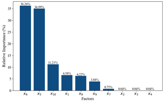
Figure 16. Relative importance of deformation feature factors.

To verify the impact of factor selection on the displacement prediction model, the deformation feature factors were sequentially input into a standard RF model in order of decreasing relative importance. Specifically, the most important feature factor was first introduced for preliminary model training and testing, followed by a gradual increase in the number of feature factors until all selected factors were included. After each addition, the Root Mean Square Error (RMSE) of both the training and test sets was calculated to quantify the model’s prediction accuracy. The final results are shown in Figure 17.

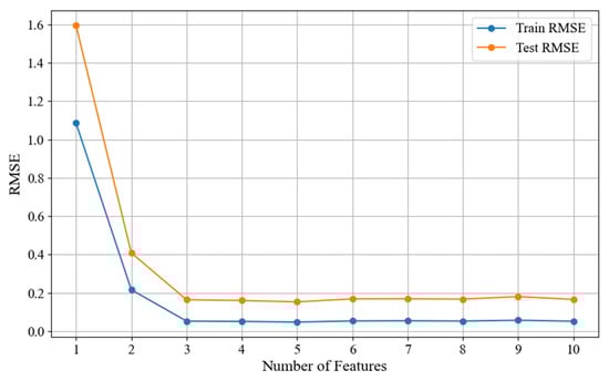
Figure 17. RMSE of the RF model with different input factors.

From Figure 17, it can be seen that as the number of input feature factors increases, the RMSE values of both the training and test sets gradually decrease and stabilize. Initially, when the number of feature factors is small, the model lacks sufficient effective input information, resulting in higher RMSE values for both sets. For instance, with only factor x₆ included, the training set RMSE is 1.0861, and the test set RMSE is 1.5959, indicating that the model fails to fully capture the nonlinear characteristics of dam deformation. As more deformation-related feature factors are added, the RMSE decreases significantly. When the number of factors reaches 5, the training set RMSE drops to 0.0473, and the test set RMSE drops to 0.1527, demonstrating a substantial improvement in model performance. However, further increasing the number of features does not lead to additional RMSE reduction; instead, a slight upward trend is observed. For example, when the number of factors increases to 9, the test set RMSE rises to 0.1802. This suggests that excessive redundant information, particularly from strongly correlated but low-importance factors (e.g., x₂ and x₃), negatively affects the model’s predictive capability.

Therefore, to ensure the input variables contain sufficient information to reflect dam deformation patterns while avoiding interference from redundancy and multicollinearity, this study selects the top 5 feature factors with the highest LASSO-based relative importance to construct a new feature subset, ${\mathit{X}}_L$, as the model input:

$${\mathit{X}}_L=\left(x_1,x_5,x_6,x_8,x_{10}\right)=\left(H,\sin {\displaystyle \frac{2\pi t}{365}},\cos {\displaystyle \frac{2\pi t}{365}},\cos {\displaystyle \frac{4\pi t}{365}},ln\theta \right)$$

(49)

4.5. Displacement Prediction Model Validation

To comprehensively evaluate the feasibility and performance of the DE-IRSA-RF model, we conducted model validation through the following steps. First, a comparative analysis was performed between the IRSA-RF model, the RSA-RF model, and the standard RF model to determine whether the IRSA-RF model exhibits superior performance over the other two. Subsequently, the DE-IRSA-RF model was compared with classical prediction models, including Multiple Linear Regression (MLR), Support Vector Regression (SVR), and Long Short-Term Memory Neural Network (LSTM), to thoroughly assess its prediction accuracy and robustness. Finally, to verify the model’s generalization capability, the performance of the DE-IRSA-RF model at monitoring points DC4 and DC5 was compared with that of the three classical prediction models.

5. Results and Discussion

5.1. Improvement Effects of IRSA-RF Model

Taking the 594 monitoring data periods from 13 January 2021 to 29 August 2022, at monitoring point DC2 as an example, the improvement effects of the IRSA-RF model over the prototype model were verified. Considering the temporal dependency of the data, the time step was selected within the range of 1 to 20 through standard RF-based hyperparameter optimization. The evaluation involved training separate RF models for each candidate time step and selecting the one with the minimum RMSE. As shown in Figure 18, the time step was ultimately set to 16 as it achieved the lowest RMSE among all candidates. The time step defines the number of consecutive daily observations used as input to predict the subsequent displacement. After data cleaning, factor screening, and time step optimization, the proposed IRSA obtained the optimal hyperparameter combination for the RF model: Ntree = 270, MaxDepth = 18, MinSplit = 2, MinLeaf = 1, and MaxFeatures = 21. Figure 19 presents the learning curve of the IRSA, and the Fitness Value represents the scaled 5-fold cross-validated MSE. In comparison, the RSA yielded hyperparameters of Ntree = 147, MaxDepth = 13, MinSplit = 2, MinLeaf = 4, and MaxFeatures = 17. Figure 20 presents the horizontal displacement prediction results of IRSA-RF, RSA-RF, and standard RF models at monitoring point DC2, while Table 8 lists the performance evaluation metrics of the three models.

Figure 18. Time step optimization for the RF model.

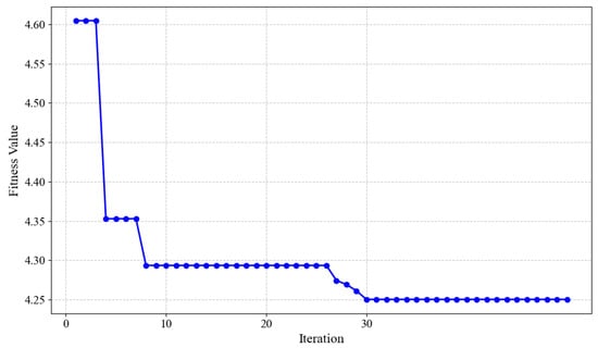
Figure 19. Iterative process diagram of the IRSA.

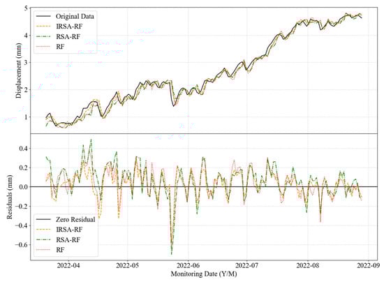
Figure 20. Predicted displacements of IRSA-RF, RSA-RF, and RF at DC2.

Table 8. Performance evaluation metrics of IRSA-RF, RSA-RF, and RF at DC2.

Monitoring Point	Model	MAE	RMSE	AEmax	R	R2
DC2	IRSA-RF	0.1025	0.1322	0.5749	0.9949	0.9891
	RSA-RF	0.1039	0.1371	0.6656	0.9943	0.9883
	RF	0.1181	0.1535	0.6700	0.9929	0.9853

As observed in Figure 20 and Table 8, after data engineering processes including KF-DTIF data cleaning and LASSO-based feature factor screening, all three RF-based models demonstrated excellent alignment with the original displacement data, with evaluation metrics falling within highly favorable ranges. Specifically, the IRSA-RF model achieved a 1.35% and 13.21% reduction in MAE compared to RSA-RF and standard RF, respectively. Similarly, RMSE decreased by 3.43% and 13.75%, while AEmax was reduced by 13.26% and 13.84%. Additionally, both R and R² showed slight improvements. These enhancements confirm the practical effectiveness of the IRSA-RF model in better adapting to the prediction requirements of dam displacement monitoring data. The results clearly demonstrate that the proposed IRSA optimization not only refines the hyperparameters but also significantly enhances the model’s predictive accuracy and reliability, making it more suitable for real-world dam displacement monitoring applications.

5.2. Prediction Performance Comparison Between DE-IRSA-RF and Classical Models

Using the dataset from monitoring point DC2, MLR, SVR, and LSTM were selected to represent traditional statistical models, classical machine learning models, and deep learning models, respectively, for comparative analysis with the proposed DE-IRSA-RF model in terms of prediction performance. The SVR model parameters were optimized through grid search, resulting in a regularization parameter c of 0.1, kernel function parameter g of 3.71, and a polynomial kernel type. The LSTM model was configured with 50 hidden neurons, the Adam optimizer, a learning rate of 0.001, 50 epochs, and a batch size of 32. Figure 21 displays the displacement time series predicted by the aforementioned models at DC2, while Table 9 presents the corresponding evaluation metrics.

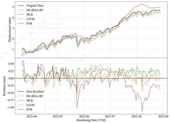
Figure 21. Predicted displacements of four models at DC2.

Table 9. Performance evaluation metrics of four prediction models at DC2.

Monitoring Point	Model	MAE	RMSE	AEmax	R	R2
DC2	DE-IRSA-RF	0.1025	0.1324	0.5773	0.9949	0.9891
	MLR	0.2153	0.2376	0.4079	0.9955	0.9648
	SVR	0.2543	0.3396	1.1422	0.9834	0.9281
	LSTM	0.2098	0.2538	0.5600	0.9842	0.9599

As shown in Figure 21, the DE-IRSA-RF model’s predictions align more closely with the original displacement curve compared to the other three classical models. The residual plot further reveals that the DE-IRSA-RF model exhibits smaller fluctuations around the zero-residual line, with both mean and maximum residuals lower than those of MLR, SVR, and LSTM. Table 9 demonstrates that the proposed DE-IRSA-RF model significantly outperforms the classical models in terms of MAE, RMSE, and AE_max. Notably, it achieves improvements exceeding 51.14% in MAE and 44.28% in RMSE compared to the best-performing alternative model. Although MLR slightly surpasses DE-IRSA-RF in the R metric by a negligible 0.06%, the latter demonstrates clear superiority in R², indicating stronger explanatory power for the data. These results confirm the superiority of the DE-IRSA-RF model over classical prediction models.

5.3. Generalization Capability Verification of DE-IRSA-RF Model

To evaluate the generalization capability of the DE-IRSA-RF model, this section compares the displacement predictions of the four models using monitoring data from points DC4 (right quarter dam beam) and DC5 (right dam abutment at the crest). For the DE-IRSA-RF model, the optimal RF hyperparameters at DC4 were Ntree = 298, MaxDepth = 9, MinSplit = 10, MinLeaf = 1, and MaxFeatures = 13, while those at DC5 were Ntree = 269, MaxDepth = 14, MinSplit = 8, MinLeaf = 2, and MaxFeatures = 8. The SVR model parameters were optimized via grid search, yielding regularization parameters c of 0.7 and 2.2 for DC4 and DC5, respectively, a kernel function parameter g of 0.01, and a linear kernel type. The LSTM hyperparameters maintained the same configuration as specified in Section 5.2. Figure 22 illustrates the displacement predictions of the four models at these points. The DE-IRSA-RF model’s predictions closely follow the actual displacement curves, with smaller residual fluctuations, demonstrating superior anti-interference and generalization capabilities. In contrast, the SVR model fails to capture sufficient displacement information at DC4, producing overly smooth predictions, while exhibiting significant deviation in the latter half of DC5 predictions, indicating poor generalization. Table 10 summarizes the corresponding evaluation metrics.

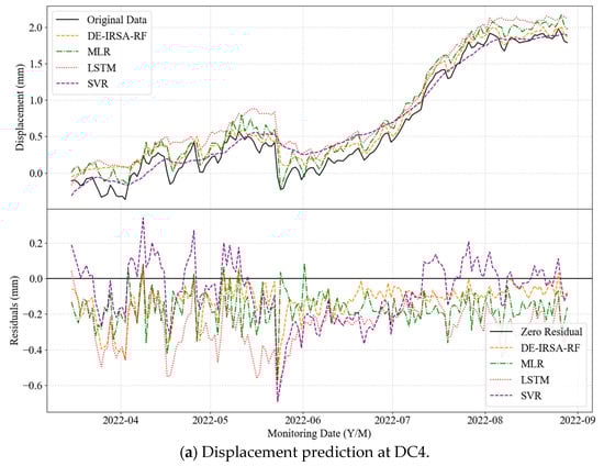
Figure 22. Predicted displacements of four models at DC4 and DC5.

Table 10. Performance evaluation metrics of four models at DC4 and DC5.

Monitoring Point	Model	MAE	RMSE	AEmax	R	R2
DC4	DE-IRSA-RF	0.0732	0.0854	0.2160	0.9873	0.9347
	MLR	0.1704	0.1902	0.5714	0.9921	0.9341
	SVR	0.1425	0.1807	0.6903	0.9763	0.9405
	LSTM	0.2195	0.2496	0.6223	0.9858	0.8866
DC5	DE-IRSA-RF	0.0753	0.0886	0.2501	0.9677	0.9298
	MLR	0.1360	0.1574	0.3936	0.9002	0.7778
	SVR	0.2008	0.2640	0.5189	0.8871	0.3751
	LSTM	0.1373	0.1535	0.2924	0.9766	0.7886

As shown in Table 10, the DE-IRSA-RF model demonstrates significant performance advantages at both monitoring points DC4 and DC5. The MAE values of the DE-IRSA-RF model are 0.0732 and 0.0753 at these two points, respectively, representing improvements of over 48.6% and 44.6% compared to the best-performing SVR and MLR models. Similarly, its RMSE outperforms the top-performing SVR and LSTM models by more than 52.7% and 42.3%, respectively. The DE-IRSA-RF model also maintains consistently high performance across other evaluation metrics. In contrast, other models exhibit notable fluctuations in various indicators across different monitoring points—for instance, the R² value of the SVR model drops sharply from 0.9405 to 0.3751, indicating poor generalization capability. The variation in R² values of DE-IRSA-RF model across monitoring points (0.9891 at DC2, 0.9347 at DC4, and 0.9298 at DC5) reflects the different structural behaviors and environmental conditions at each location. While DC2 exhibits more predictable thermal displacement patterns, DC4 and DC5 are influenced by complex foundation-abutment interactions that introduce additional nonlinearities. Nevertheless, the DE-IRSA-RF model maintains strong performance at all locations, demonstrating its robustness and adaptability to varying structural conditions.

Overall, the DE-IRSA-RF model excels in prediction accuracy, correlation, and generalization performance compared to other models. Particularly when handling complex data, it maintains high stability and precision, making it well-suited for practical engineering applications in displacement prediction tasks.

6. Conclusions

This study proposes a two-phase dam displacement analysis model, the DE-IRSA-RF model, which integrates an improved iForest with metaheuristic-optimized RF to address the challenge of balancing data quality and prediction accuracy in traditional dam displacement monitoring models. Through validation with engineering case studies, the model demonstrates significant advantages in both anomaly detection and displacement prediction, providing reliable technical support for dam structural safety monitoring. The main conclusions of this research are as follows:

(1)

The data-cleaning strategy combining KF and DTIF effectively removes noise and outliers from monitoring data. KF suppresses noise through recursive estimation and residual correction, while DTIF enhances anomaly detection accuracy and robustness via an adaptive threshold mechanism. Experimental results show that DTIF achieves superior detection precision across various outlier distribution scenarios, ensuring high-quality input data for subsequent prediction models.

(2)

Based on the HST statistical model, the LASSO algorithm was employed to analyze and screen the importance of displacement feature factors, extracting an optimal feature subset as model input to minimize interference from redundant factors. Case studies confirm that the model with feature selection achieves significant improvements in both prediction accuracy and generalization capability.

(3)

The IRSA enhances the standard RSA by incorporating Tent chaotic mapping, dynamic parameters, Lévy flight strategy, and EOBL, thereby improving global search capability and local exploitation precision while avoiding premature convergence and local optima. A comparison between RF and RSA-RF demonstrates that the IRSA-RF model significantly reduces prediction errors in long-term displacement forecasting tasks.

(4)

Compared to classical models such as MLR, SVR, and LSTM, the DE-IRSA-RF framework exhibits superior performance in displacement prediction tasks across different monitoring points. Its strong generalization ability and high prediction accuracy highlight its potential as a reliable tool for early risk warning and decision-making in dam safety monitoring.

Future research will focus on two key extensions of this work: (i) generalizing the framework from single-point to spatiotemporal analysis of multiple monitoring points to enhance robustness, and (ii) expanding the benchmark suite to include state-of-the-art ensemble models like XGBoost and LightGBM for more comprehensive validation.

References

- Huang, M.; Wan, N.; Zhu, H. Reconstruction of structural acceleration response based on CNN-BiGRU with squeeze-and-excitation under environmental temperature effects. J. Civ. Struct. Health Monit. 2024, 15, 985–1003. [Google Scholar] [CrossRef]
- Zhang, J.; Huang, M.; Wan, N.; Deng, Z.; He, Z.; Luo, J. Missing measurement data recovery methods in structural health monitoring: The state, challenges and case study. Measurement 2024, 231, 114528. [Google Scholar] [CrossRef]
- Deng, Z.; Gao, Q.; Huang, M.; Wan, N.; Zhang, J.; He, Z. From data processing to behavior monitoring: A comprehensive overview of dam health monitoring technology. Structures 2025, 71, 108094. [Google Scholar] [CrossRef]
- Duffaut, P.; Larouzée, J. Geology, Engineering & Humanities: 3 sciences behind the Malpasset dam failure (France, Dec. 2, 1959). Q. J. Eng. Geol. Hydrogeol. 2019, 52, 445–458. [Google Scholar]
- Zipper, M.; Zulauf, N.; Bendels, M.H.K. The Banqiao Dam catastrophe. Zentralblatt Arbeitsmedizin Arbeitsschutz Ergon. 2020, 70, 230–235. [Google Scholar] [CrossRef]
- Guo, Y.; You, Z.; Wei, B. Working Mode Identification Method for High Arch Dam Discharge Structure Based on Improved Wavelet Threshold-EMD and RDT Algorithm. Water 2022, 14, 3735. [Google Scholar] [CrossRef]
- Deng, Z.; Huang, M.; Wan, N.; Zhang, J. The Current Development of Structural Health Monitoring for Bridges: A Review. Buildings 2023, 13, 1360. [Google Scholar] [CrossRef]
- Su, H.; Chen, J.; Wen, Z.; Wang, F. Wavelet-fractal diagnosis model and its criterion for concrete dam crack status. Trans. Inst. Meas. Control 2018, 40, 1846–1853. [Google Scholar] [CrossRef]
- Su, H.; Li, H.; Chen, Z.; Wen, Z. An approach using ensemble empirical mode decomposition to remove noise from prototypical observations on dam safety. Springerplus 2016, 5, 650. [Google Scholar] [CrossRef] [PubMed]
- Jia, D.; Yang, J.; Sheng, G. Dam deformation prediction model based on the multiple decomposition and denoising methods. Measurement 2024, 238, 115268. [Google Scholar] [CrossRef]
- Khodarahmi, M.; Maihami, V. A Review on Kalman Filter Models. Arch. Comput. Methods Eng. 2023, 30, 727–747. [Google Scholar] [CrossRef]
- Dai, W.; Liu, N.; Santerre, R.; Pan, J. Dam Deformation Monitoring Data Analysis Using Space-Time Kalman Filter. ISPRS Int. J. Geo-Inf. 2016, 5, 236. [Google Scholar] [CrossRef]
- Li, B.; Yang, J.; Hu, D. Dam monitoring data analysis methods: A literature review. Struct. Control Health Monit. 2020, 27, e2501. [Google Scholar] [CrossRef]
- Liu, F.T.; Ting, K.M.; Zhou, Z.-H. Isolation forest. In Proceedings of the 2008 Eighth IEEE International Conference on Data Mining, Pisa, Italy, 15–19 December 2008; pp. 413–422. [Google Scholar]
- Karczmarek, P.; Kiersztyn, A.; Pedrycz, W.; Al, E. K-Means-based isolation forest. Knowl.-Based Syst. 2020, 195, 105659. [Google Scholar] [CrossRef]
- Hariri, S.; Kind, M.C.; Brunner, R.J. Extended Isolation Forest. IEEE Trans. Knowl. Data Eng. 2021, 33, 1479–1489. [Google Scholar] [CrossRef]
- Lesouple, J.; Baudoin, C.; Spigai, M.; Tourneret, J.-Y. Generalized isolation forest for anomaly detection. Pattern Recognit. Lett. 2021, 149, 109–119. [Google Scholar] [CrossRef]
- Yu, Y.; Liu, X.; Wang, E.; Fang, K.; Huang, L. Dam Safety Evaluation Based on Multiple Linear Regression and Numerical Simulation. Rock Mech. Rock Eng. 2018, 51, 2451–2467. [Google Scholar] [CrossRef]
- Shao, C.; Gu, C.; Meng, Z.; Hu, Y. Integrating the Finite Element Method with a Data-Driven Approach for Dam Displacement Prediction. Adv. Civ. Eng. 2020, 2020, 4961963. [Google Scholar] [CrossRef]
- Ma, B.; Zhou, J.; Zhang, C. Risk Prediction Model for Tailings Ponds Based on EEMD-DA-LSTM Model. Appl. Sci. 2024, 14, 9141. [Google Scholar] [CrossRef]
- Wan, N.; Huang, M.; Lei, Y. High-efficiency finite element model updating of bridge structure using a novel physics-guided neural network. Int. J. Struct. Stab. Dyn. 2024, 2650006. [Google Scholar] [CrossRef]
- Kao, C.-Y.; Loh, C.-H. Monitoring of long-term static deformation data of Fei-Tsui arch dam using artificial neural network-based approaches. Struct. Control Health Monit. 2013, 20, 282–303. [Google Scholar] [CrossRef]
- Wang, S.; Zhuang, J.; Zheng, J.; Fan, H.; Kong, J.; Zhan, J. Application of Bayesian Hyperparameter Optimized Random Forest and XGBoost Model for Landslide Susceptibility Mapping. Front. Earth Sci. 2021, 9, 617. [Google Scholar] [CrossRef]
- Zhu, N.; Zhu, C.; Zhou, L.; Zhu, Y.; Zhang, X. Optimization of the Random Forest Hyperparameters for Power Industrial Control Systems Intrusion Detection Using an Improved Grid Search Algorithm. Appl. Sci. 2022, 12, 10456. [Google Scholar] [CrossRef]
- Gu, C.; Wu, B.; Chen, Y. A High-Robust Displacement Prediction Model for Super-High Arch Dams Integrating Wavelet De-Noising and Improved Random Forest. Water 2023, 15, 1271. [Google Scholar] [CrossRef]
- Huang, M.; Zhang, J.; Hu, J.; Ye, Z.; Deng, Z.; Wan, N. Nonlinear modeling of temperature-induced bearing displacement of long-span single-pier rigid frame bridge based on DCNN-LSTM. Case Stud. Therm. Eng. 2024, 53, 103897. [Google Scholar] [CrossRef]
- Huang, M.; Zhang, J.; Li, J.; Deng, Z.; Luo, J. Damage identification of steel bridge based on data augmentation and adaptive optimization neural network. Struct. Health Monit.-Int. J. 2024, 24, 1674–1699. [Google Scholar] [CrossRef]
- Huang, M.; Ling, Z.; Sun, C.; Lei, Y.; Xiang, C.; Wan, Z.; Gu, J. Two-stage damage identification for bridge bearings based on sailfish optimization and element relative modal strain energy. Struct. Eng. Mech. 2023, 86, 715–730. [Google Scholar]
- Abualigah, L.; Abd Elaziz, M.; Sumari, P.; Geem, Z.W.; Gandomi, A.H. Reptile Search Algorithm (RSA): A nature-inspired meta-heuristic optimizer. Expert Syst. Appl. 2022, 191, 116158. [Google Scholar] [CrossRef]
- Adnan, R.M.; Mostafa, R.R.; Dai, H.-L.; Heddam, S.; Masood, A.; Kisi, O. Enhancing accuracy of extreme learning machine in predicting river flow using improved reptile search algorithm. Stoch. Environ. Res. Risk Assess. 2023, 37, 3063–3083. [Google Scholar] [CrossRef]
- Almotairi, K.H.; Abualigah, L. Hybrid Reptile Search Algorithm and Remora Optimization Algorithm for Optimization Tasks and Data Clustering. Symmetry 2022, 14, 458. [Google Scholar] [CrossRef]
- Otsu, N. Threshold selection method from gray-level histograms. IEEE Trans. Syst. Man Cybern. 1979, 9, 62–66. [Google Scholar] [CrossRef]
- Leger, P.; Leclerc, M. Hydrostatic, temperature, time-displacement model for concrete dams. J. Eng. Mech. 2007, 133, 267–277. [Google Scholar] [CrossRef]
- Wang, S.; Xu, C.; Gu, C.; Su, H.; Wu, B. Hydraulic-seasonal-time-based state space model for displacement monitoring of high concrete dams. Trans. Inst. Meas. Control 2021, 43, 3347–3359. [Google Scholar] [CrossRef]
- Yang, G.; Gu, H.; Chen, X.; Zhao, K.; Qiao, D.; Chen, X. Hybrid hydraulic-seasonal-time model for predicting the deformation behaviour of high concrete dams during the operational period. Struct. Control Health Monit. 2021, 28, e2685. [Google Scholar] [CrossRef]
- Liu, X.; Li, Z.; Sun, L.; Khailah, E.Y.; Wang, J.; Lu, W. A critical review of statistical model of dam monitoring data. J. Build. Eng. 2023, 80, 108106. [Google Scholar] [CrossRef]
- Mata, J.; Tavares de Castro, A.; Sá da Costa, J. Constructing statistical models for arch dam deformation. Struct. Control Health Monit. 2014, 21, 423–437. [Google Scholar] [CrossRef]
- Willm, G.; Beaujoint, N. Les méthodes de surveillance des barrages au service de la production hydraulique d’Electricité de France, problèmes anciens et solutions nouvelles. In Proceedings of the IXth International Congress on Large Dams, Istanbul, Turkey, 4–8 September 1967; pp. 529–550. [Google Scholar]
- Tibshirani, R. Regression shrinkage and selection via the lasso: A retrospective. J. R. Stat. Soc. Ser. B Stat. Methodol. 2011, 73, 273–282. [Google Scholar] [CrossRef]
- Breiman, L. Random forests. Mach. Learn. 2001, 45, 5–32. [Google Scholar] [CrossRef]
- Probst, P.; Wright, M.N.; Boulesteix, A.-L. Hyperparameters and tuning strategies for random forest. Wiley Interdiscip. Rev. Data Min. Knowl. Discov. 2019, 9, e1301. [Google Scholar] [CrossRef]
- Sasmal, B.; Hussien, A.G.; Das, A.; Dhal, K.G.; Saha, R. Reptile Search Algorithm: Theory, Variants, Applications, and Performance Evaluation. Arch. Comput. Methods Eng. 2024, 31, 521–549. [Google Scholar] [CrossRef]
- Li, Y.; Han, M.; Guo, Q. Modified Whale Optimization Algorithm Based on Tent Chaotic Mapping and Its Application in Structural Optimization. KSCE J. Civ. Eng. 2020, 24, 3703–3713. [Google Scholar] [CrossRef]
- Hakli, H.; Uguz, H. A novel particle swarm optimization algorithm with Levy flight. Appl. Soft Comput. 2014, 23, 333–345. [Google Scholar] [CrossRef]
- Yildiz, B.S.; Pholdee, N.; Bureerat, S.; Yildiz, A.R.; Sait, S.M. Enhanced grasshopper optimization algorithm using elite opposition-based learning for solving real-world engineering problems. Eng. Comput. 2022, 38, 4207–4219. [Google Scholar] [CrossRef]
Disclaimer/Publisher’s Note: The statements, opinions and data contained in all publications are solely those of the individual author(s) and contributor(s) and not of MDPI and/or the editor(s). MDPI and/or the editor(s) disclaim responsibility for any injury to people or property resulting from any ideas, methods, instructions or products referred to in the content. |
© 2025 by the authors. Licensee MDPI, Basel, Switzerland. This article is an open access article distributed under the terms and conditions of the Creative Commons Attribution (CC BY) license (https://creativecommons.org/licenses/by/4.0/).