Abstract
In current practice, the deployment of artificial intelligence models for the optimization of construction processes is highly complex and limited, primarily due to the lack of data available for training models. Collecting real-world data is both time-consuming and resource-intensive. This paper focuses on the development of a methodology and a model for generating synthetic data intended for the subsequent training of artificial intelligence models for optimizing construction machinery assemblies. The proposed synthetic data generation process is based on simulation principles that employ queuing theory and the stochastic Monte Carlo method. This approach enables the rapid creation of large-scale synthetic datasets. The developed model and generator are specifically focused on the use of construction machinery in earthworks. Selected generated data were compared with and validated against real construction projects. The synthetic data demonstrated very good agreement with the observed data across key performance indicators. For Total Cost, CO2 Emissions, Fuel Consumption, and Completion Time, deviations between synthetic and real project data were generally within 5–7%, which is considered acceptable for construction process simulations. In contrast, the Number of Failures exhibited noticeably higher deviations (approximately 10–15%), indicating the current model’s weaker predictive capability for this metric. The outcomes of this study can benefit contractors and construction equipment manufacturers by improving design efficiency, reducing costs, and enhancing machine performance.
1. Introduction
1.1. General Background
The construction industry is a highly significant sector of the national economy and an integral part of everyday human life [1,2]. Since the emergence of humankind, construction technologies have continuously evolved—from simple methods, such as the construction of a hut, to the highly complex processes involved in the construction of a nuclear power plant [3]. The capabilities of modern computing technology are nearly limitless regarding volume, storage duration, and the preservation of essential information for future generations [4]. At the same time, humanity faces a profound challenge—one that is nearly insurmountable given the limits of the human brain: to navigate, comprehend, and effectively utilize the vast amount of complex information available [5].
Modern construction technologies are the result of a synthesis of various scientific disciplines (mathematics, physics, chemistry, economics, etc.) [6]. The modeling and optimization of construction processes are indispensable for improving construction outputs and must rely on proven methods, procedures, and AI [7]. The integration of complex and diverse construction indicators (e.g., activities; labor, energy, and material resources) into a mathematical–technological AI model requires knowledge of specific technical capabilities, mathematical methods, and precise algorithms [7]. Errors, inaccuracies, or inefficient sequencing of processes in a construction–technological project may affect the entire life cycle of a building [8].
Construction production is typically an individualized process, carried out under specific conditions and constraints (terrain, local, climatic, economic, technological, legal, etc.) [6]. Even minor oversight or failure to consider decisive or less evident factors can render a project suboptimal regarding economic, technological, environmental, or occupational health and safety outcomes [8]. This reality underscores the urgent need to optimize construction processes and to select optimal mechanized equipment assemblies for the execution of construction works [9].
A construction project for a complex building may involve hundreds or even thousands of individual process items, each containing highly sophisticated information (productivity, costs, environmental impacts, interdependencies, safety risks, probability of equipment failure, fuel consumption, CO2 emissions, process durations, etc.) [7]. Simulation processes often fail due to the enormous computational power required, making it impossible to achieve complete coverage of all processes and alternatives [9]. Predictive AI models operate with a certain degree of accuracy; although the results may not be globally optimal, they can significantly and rapidly improve the efficiency of the entire process [10]. Without the use of AI models, optimization steps cannot be effectively undertaken, efficiency in construction production cannot be increased, and the negative environmental impacts of construction cannot be mitigated [10].
1.2. Literature Review
The field of production process optimization is widely studied, while the application of AI in the optimization of construction processes is still developing. Both researchers and construction companies continue to develop AI models and seek effective methods for their implementation in practice. Considerable research has been devoted to the modeling of construction production and the application of mathematical methods in construction. The origins of scientific inquiry in this field date back to the early 20th century, when, following the Industrial Revolution, problems of labor efficiency became highly relevant. The development of mathematical and subsequent economic frameworks enabled the evolution of optimization methods [11,12,13]. Initially, simple methods and applications were employed, but with advances in modern computing, increasingly complex and powerful mathematical methods and optimization algorithms emerged.
The topic of mathematical modeling in construction has been addressed in various ways. In the United States, Luenberger [14] laid the theoretical foundations for optimization through his work on linear and nonlinear programming, which became fundamental to later applications in engineering and construction management. Ackoff and Sasieni [15] contributed to the development of operations research and its use in decision-making and planning of complex industrial and construction processes.
In the Czech Republic, Jarský [16,17] conducted pioneering research on the mathematical modeling of construction processes and later introduced automation in the planning and management of construction projects. His work established algorithmic and computer-assisted approaches to process organization and optimization in construction practice. Motyčka et al. [18] extended these concepts through empirical studies, focusing on the effective utilization of construction machinery—specifically tower cranes—based on time efficiency and productivity analyses.
In Slovakia, Břoušek, Vávra, and Zapletal [19] contributed to the field through their work on construction technology for civil engineering structures, emphasizing the technological and organizational aspects of construction production. Tažiková, Struková, and Kozlovská [20] further advanced this area by analyzing real operation times on construction sites, highlighting data-driven optimization of workflows and equipment usage in residential building projects.
In Russia, Puchov and Chatiashvili [21] developed mathematical models of technological processes aimed at improving the organization and efficiency of construction production. Their research was complemented by Pontrjagin [22], whose mathematical theory of optimal processes provided the theoretical background for optimization problems later adapted to mechanized equipment assemblies and construction process control.
In Lithuania, Zavadskas [23] explored construction modeling and the application of computer systems. Jarský made a significant contribution by introducing an automated computer system into construction practice [24]. Additional international sources [25,26,27,28,29,30,31] also provided valuable inspiration for this research. Based on an analysis of the current state of the field and a thorough review of the literature, suitable methods for AI-based modeling of construction processes and identification of optimal equipment assemblies were selected.
Numerous systems for the planning of construction processes exist (e.g., Primavera P6 Professional 24, Procore Preconstruction 2025, Aconex Oracle 25, MS Project Professional 2024). Most software tools rely on relatively simple mathematical models of network diagrams to identify the critical path and optimize the allocation of resources. However, the area of optimal selection of mechanized equipment assemblies is still in its early stages, and software tools enabling the easy optimization of equipment selection (considering minimization of labor and costs, fuel consumption, construction duration, environmental impacts, etc.), along with the corresponding data, are currently unavailable. The application of AI for identifying the most efficient equipment assembly for specific tasks is entirely lacking.
The principal barrier to the implementation of AI models in construction practice is the critical lack of high-quality training data. The acquisition of reliable data records is both time- and cost-intensive, posing a substantial obstacle to large-scale implementation. Training AI models requires vast datasets composed of structured and validated information. For predictive and optimization models to achieve high accuracy, datasets containing millions of records are indispensable [32]. According to [33,34], the collection of a single record from existing construction projects may represent as much as 2–3% of the overall project cost and, on average, may require up to three months. As a result, the training of AI models for the optimization of construction machinery on real-world data becomes impractical. Consequently, the only viable pathway is the development of a synthetic data generator [35], capable of producing the necessary datasets for subsequent model training.
1.3. Research Gap
A detailed review of the existing literature and scientific publications revealed that a clearly defined and comprehensive methodology for generating synthetic data in the context of construction machinery assemblies is currently lacking. Considering the growing adoption of artificial intelligence (AI) systems, there is an urgent need to establish a well-structured simulation process that can be potentially replicated across other industrial sectors and adapted to different problem domains.
1.4. Research Aim and Objectives
This article primarily addresses the mathematical modeling of a construction production system for synthetic data generation for AI-driven optimization of construction machinery assemblies. The developed mathematical model, including the associated databases of mechanized equipment assemblies and the environmental impacts of construction production, is intended to enable modeling, simulation, and selection of the optimal mechanized assemblies. Synthetic data for AI training were generated for different construction equipment assemblies using queuing theory [36], stochastic modeling with the Monte Carlo method [37], and multi-criteria decision-making methods. For greater credibility, synthetic data must be validated and compared against real-world data collected from actual construction projects.
In ref. [32], the authors describe a methodology for collecting and verifying synthetic data. Our primary objective is to apply this method to construction processes and to develop a sophisticated mathematical model for data simulation. In ref. [38], the authors address the use of synthetic data in the context of network management and analysis. Many authors [39,40,41,42] have investigated the use of synthetic data in construction; however, their research has been limited to autonomous construction machinery without addressing the optimization of task competition or the number of units employed. The main objective of the work in ref. [43] was to generate synthetic data for evaluating and monitoring the performance of construction works, without application to the selection of an optimal construction assembly.
1.5. Novelty and Contribution
In response to the persistent challenge of limited and costly real-world data in the construction industry, this study proposes a novel methodology for generating synthetic data to support the training of optimization models for construction machinery assemblies. The proposed approach integrates queuing theory with stochastic Monte Carlo simulation to efficiently produce realistic, large-scale datasets that capture the variability and uncertainty of construction operations. The developed model and data generator were validated against real construction project data, demonstrating their ability to provide a practical and scalable solution for reducing data collection costs and enhancing the design efficiency and operational performance of construction machinery, particularly in earthwork processes.
1.6. Structure of the Paper
The proposed model determines the mechanized equipment assembly for a given task (defined by the task volume and specific technological requirements) with respect to multiple criteria: price, costs, profit, labor intensity, fuel consumption, construction duration, environmental impact, and equipment failure rates. Section 2 describes the model for generating synthetic data. Section 3 includes verification of the model on a real construction project, which involved the collection of statistical data on the progress of construction (temporal data on machine movement within the construction site), the modeling and simulation of synthetic system data, and subsequent comparison of the simulation results. Finally, this article summarizes the main contributions of the developed model, discusses its limitations and critical points, and proposes future directions for improving the model.
2. Methods and Models
In this section, important methods and theories in the fields of mathematics, economics, and technology that were employed in the development of the proposed system will be described.
Construction production involves a highly complex integration of diverse construction processes. The individual processes are interconnected in various ways and operate within their specific limits under given conditions. It is evident that the construction production system cannot be precisely and fully described or transferred into a computational form due to its sophisticated nature. The system must therefore be simplified to the extent that it enables its straightforward implementation into a mathematical model, while ensuring that the accuracy of representation affects the modeling results only within a certain small permissible deviation.
There are numerous approaches to the mathematical modeling of construction processes, reflecting the diversity and complexity of the systems involved. These models can generally be classified as deterministic [14], such as linear programming or critical path analysis; stochastic, including Monte Carlo simulation [37], queuing theory [36], and Markov chain models [13]; or hybrid, which integrate simulation with optimization techniques or machine learning algorithms. Markov chain models are valuable for capturing state-dependent and sequential behaviors—for example, equipment operations, system reliability, and transitions between different construction states over time. Each model provides a formalized representation of a process by defining its specific input and output parameters, boundary conditions, and optimization criteria from a particular analytical perspective [44].
Each mathematical model examined in this study constitutes an isomorphic representation of a real physical object, incorporating certain abstractions that simplify the model and emphasize selected properties and parameters (see Figure 1). In isomorphic systems, the mapping of elements from one system S1 to another system S2 is bijective, and the number of nodes, edges, and their degrees is identical. This condition fully satisfies the requirements of accurate modeling of construction technological processes.
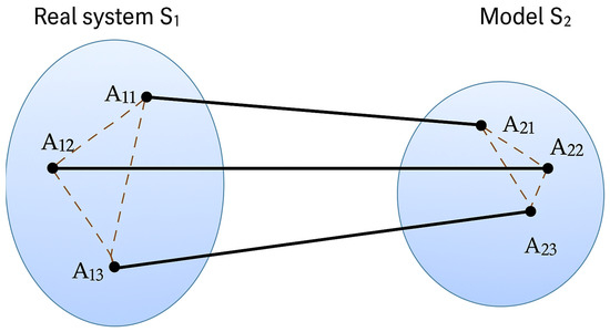
Figure 1.
Isomorphic representation of real and model systems.
The modeling of construction processes has two important aspects. The first aspect is the formal mathematical one, which precisely describes the objects entering the system (relations, constraints). Any formal system is a simplification (an idealized conception) of a real object. Consequently, for modeling, the second aspect—interpretation—is indispensable. In other words, it is necessary to define in advance the procedures for the transition between a real object and a model (input → model) and between a model and the result of modeling (model → output).
If many mathematical models of the same technological process are available, the designer or contractor will face the problem of choosing the most appropriate one. Bellman’s principle of optimality [45] states the following: “An optimal policy has the property that, whatever the initial state and initial decision are, the remaining decisions must constitute an optimal policy with regard to the state resulting from the first decision.” This principle is applied in dynamic programming and, with a certain degree of reliability, can also be employed in AI modeling and decision-making when selecting the optimal machine configuration.
The process of AI-based modeling and simulation of construction processes can be summarized in four fundamental phases in a linear process flow diagram (see Figure 2).
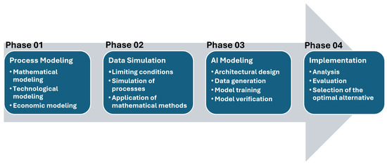
Figure 2.
Linear process flow diagram of AI modeling and simulation of construction processes.
- Phase 01: The modeling of construction processes (mathematical, economic, and technological analysis of the problem, as well as the analysis of the social behavior of the production system).
- Phase 02: The simulation of synthetic data for AI training (the definition of limiting constraints, the application of mathematical methods such as queueing theory and the Monte Carlo method, and the simulation of processes).
- Phase 03: AI modeling (design of architecture and neural network, generation of synthetic data, training, and verification).
- Phase 04: The implementation of the AI model (analysis, evaluation of results, and selection of the optimal variant).
During the first step, a detailed economic, mathematical, and technological analysis of the problem was carried out. This study considers the market of production inputs in the construction industry from both macroeconomic and microeconomic perspectives. Resources are limited at both the global and local level. The price of energy and production input for the construction production process continues to rise. Therefore, the contractor must place greater emphasis on the efficient management and utilization of the available production factors. Implementing optimization steps in the selection of machine configurations is an indispensable requirement for the effective management of a construction company and for maintaining its competitiveness in the market. Economists generally assume that the primary objective of a company is the maximization of profit (the maximization of the difference between revenues and costs) [46]. The optimal arrangement of machine configurations, not only regarding construction speed but also regarding the minimization of costs and other parameters, is highly beneficial and efficient, particularly due to the significant share of mechanized work in production.
The definition of a production function must be expressed as the relationship between the factor inputs into the system and the maximum volume of outputs over a given period [46]. The production function is expressed as follows:
where Q is the output per unit of time [units/sec], K is a production factor of capital (machinery, technology), and L is a production factor of labor (human activity).
For the analysis of the entire system, it is possible to construct an isoquant that describes all combinations of different inputs which result in the production of the same output (see Figure 3).
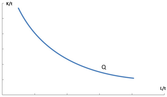
Figure 3.
Graphical representation of production isoquant.
Each point on this curve represents a combination of different labor and capital factors. For each combination of factors, there is a specific and precise calculable criterion value according to which optimization will be carried out. Any machine assembly examined during the modeling process has certain properties and parameters (performance, cost of use, fixed and variable costs, constraints, failure rate, fuel consumption, CO2 emissions). The smooth course of an isoquant is an ideal case, which does not occur due to the limitations of the production system and the factor market; in practice, it is a series of discrete points located in the vicinity of the curve. The downward slope of the isoquant describes the marginal rate of technical substitution (MRTS) and clearly determines the extent to which a construction company can change and substitute inputs without altering the level of outputs.
The main optimization task from an economic perspective was to develop an AI model that enables the rapid selection of the optimal input combination and the production of a given output at minimal cost with respect to the production function Q (1). The adjusted production function for a single construction technological process and one construction–technological crew (operating and operated resource) is expressed as follows:
where is the output per unit of time per construction technology crew [units/sec], is the serving production factor of capital (resource), and is the served production factor of capital (resource).
The graph of the production isoquant (Figure 3) can be adjusted to illustrate the dependence between the marginal product and the serving/served resource. For an unambiguous determination of the optimum cost, it is necessary for each variant to define an isocost (Figure 4), which specifies all combinations of inputs that can be acquired for a given total cost (the minimum permissible for the respective variant). The entire set of machine configurations can be expressed in vector form:
where is the total set of machine configurations, is the set of serving machine configurations and is the set of served machine configurations.
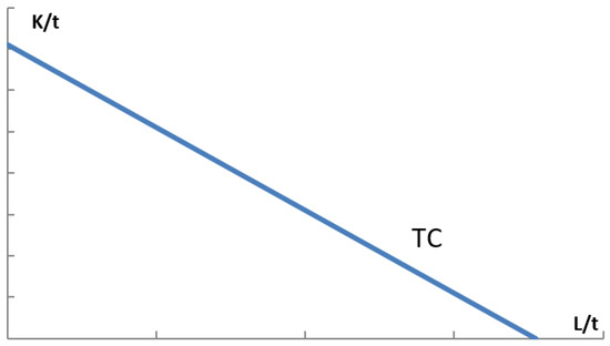
Figure 4.
Graphical representation of production isocost.
Each vector of a machine configuration is associated with additional parameters: price, costs, fuel consumption, CO2 emissions, performance, failure rate, etc. For every analyzed variant, it is possible to construct the corresponding isoquant and isocost.
The entire set of isoquant and isocost curves uniquely describes two mutually tangent surfaces and the corresponding optimal points. In Figure 5, a continuous ideal surface of the production function (the set of isoquant curves) is schematically illustrated. The total costs, according to the isocost graph, for a given analyzed variant are described by the following formula:
where is the total cost, is the number of units of serving resources, is the number of units of served resources, is the cost of one unit of the serving resource, and is the cost of one unit of the served resource.
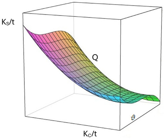
Figure 5.
A schematic representation of the continuous ideal surface of the production function.
In Figure 5, the local and global extrema that determine the optimal points of the mathematical model are evident. When the constraining conditions are incorporated into the graph, the mathematical problem becomes unambiguously defined, and the optimum cost within the examined range can be determined. It is evident that every company behaves in the market according to the well-known Least Cost Rule and seeks an optimal point within the entire feasible solution set. The developed AI model will be capable of rapidly identifying one of the optimal points which, although not necessarily global, will nevertheless be highly efficient.
The following explanation contains the mathematical derivation of the marginal rate of technical substitution (MRTS) and the determination of the optimal combination of inputs [46]. The long-run production function is expressed by Relation (2). The marginal products (MPs) of the serving and served capital resources are defined as follows:
The change in output resulting from the simultaneous variation in both inputs is given by the total differential of the production function (2):
By substituting (5) into (6), we obtain the following:
If we move along the graph of a single isoquant while changing the combination of inputs, the output remains constant, i.e., . Then, we obtain the following:
which can be rearranged as follows:
Further manipulation yields the marginal rate of technical substitution (MRTS) for an infinitesimal change in inputs such as the ratio of their marginal products:
where is the marginal rate of technical substitution between the serving and served capital resources.
To determine the optimal combination of inputs, the Lagrange multiplier () method is applied. The cost optimum can be formulated in two ways: either as the minimization of costs for a given output level or as the maximization of output for given costs. Each formulation requires the construction of a specific Lagrangian.
For the case illustrated by the isoquant , where the objective is to minimize costs for a specified output, the Lagrangian is constructed as follows:
The necessary conditions to obtain the minimum are as follows:
Solving this system yields the minimum values of and required to produce . From Equations (10) and (11), we isolate λ as follows:
Thus, the following must hold:
which can be rearranged as follows:
For the case illustrated by the isocost , the objective is to determine the number of inputs that the firm must purchase to achieve the required output under the following constraint:
The second Lagrangian is formulated as follows:
The first-order conditions are as follows:
From the first and second conditions, we obtain the following:
The following holds:
which can be rearranged as follows:
Thus, the cost optimum is defined as follows:
where is the price of one unit of the serving resource and is the price of one unit of the served resource.
The analysis of the economic model and key simulation parameters revealed the presence of both global and local minima and maxima within the entire set of feasible solutions, which can be identified during the simulation process of machine assemblies. The economic model is integrated into the simulation procedure, as illustrated in the algorithm’s pseudo-code (see Appendix B), and is employed for evaluating the total system costs. For simplification purposes, certain economic assumptions and influences were omitted in the model simulation (e.g., additional costs associated with newly acquired resources and the supply–demand relationship for resources). These factors and relationships may be explored in future research and are further discussed in the Discussion Section. Incorporating extended economic parameters is expected to enhance the algorithm’s accuracy and reduce deviations between synthetic and real-world data.
Construction production is a process composed of numerous activities. Each construction activity is subject to limiting boundaries: space, time, and technology. Construction management should rationally select the necessary production factor, considering not only the above-mentioned parameters but also the economic aspects. Each production factor has its own performance and specific parameters (e.g., minimum working area, reach, fuel and water consumption, repair and maintenance), as well as one-time acquisition costs (transportation to and from the construction site, installation and removal of equipment, worker training, i.e., the so-called initial entry into the work task). Moreover, each production indicator has its own work schedule.
A production factor can fulfill a construction task only if certain technological constraints are satisfied. Construction production is not standardized; each construction project is, in its own way, unique. It is executed according to a specific project and under varying geographical, climatic, and situational conditions. Technological constraints are clearly defined by the boundaries of technological feasibility. Every technology requires strict adherence to an exact technological procedure, which subsequently determines the requirements for the type of production factor, the duration of the process, and the climatic and external conditions (i.e., standardized conditions at the workplace). In certain cases, technological constraints may become dominant and decisive for the selection of a production factor. Technological capabilities can generally be extended only at additional costs (e.g., the use of special concrete additives for winter construction). These additional costs may be interpreted either as a specific process that shortens the technological downtime or, from the cost perspective, as a coefficient that increases the efficiency of the production factor. Safety requirements can also be included, as they define the lower and upper limits for the number of machines or crews.
The contractor usually has only a limited working area—the construction site—and must cope with a wide range of concurrent construction processes in various terrain conditions. These processes often intersect and interfere with one another. Furthermore, each production indicator requires a minimum working space on the site. The ratio of the minimum working space to the total working space for a given production factor determines the working front coefficient, one of the fundamental limiting parameters in the spatial structure of a construction project. The minimum working front defines the lower boundary of the number of machines or crews that construction management can allocate to complete a given task [47]. The working front coefficient is calculated according to Equation (18) and is usually expressed as a percentage.
where is the working queue coefficient [%], is the minimum working queue, and is the total working queue.
Another important concept is labor productivity (sometimes referred to as the norm of output), which is determined as the volume of production of a given process produced per unit of time, according to Equation (19) [47]:
where is the labor productivity [], is the production output resulting from a given process, expressed in physical or monetary units [units], and is the time in temporal units (typically hours).
The time norm specifies, in time units (minutes, hours, etc.), how much time a worker or crew requires to complete a given task (e.g., processing, transport, execution) [47].
The actual labor input is the total amount of work required to produce a certain quantity of output from a specific process. It is calculated according to Equation (20) and is measured in labor hours [47]:
where is the actual labor input [], is the production output resulting from a given process, expressed in physical or monetary units [units], is the time norm, i.e., the standard consumption of working time of one worker or one machine per unit of output [hours/units], and is the norm intensity coefficient (the ratio between the actual and standard labor input of a given process).
The duration of a partial process can be calculated using the following equation:
where is the duration of a partial construction process in days [days]; is the actual labor input [hours]; is the number of workers or machines in mechanized construction processes; is the number of working hours per shift [hours/shift]; and is the shift factor, i.e., the number of shifts per day.
In the second step, the model generates synthetic data required for the training process of the AI model and calculates the number of necessary resource units under the assumption that the resources assigned to the task operate according to a uniform work schedule (work contour: flat). Based on the findings in ref. [17], the following mathematical methods and theories were applied: queueing theory and Monte Carlo.
Queueing theory (theory of mass service) deals with the study of systems with service channels, where queues are formed and subsequently serviced by service centers. The primary objective of queueing theory is to determine the laws governing the functioning of the system and to develop the most accurate possible mathematical model that accounts for various probabilistic factors influencing the entire process [45,48].
A construction process can be examined both from the perspective of the customer waiting in line, who is primarily interested in the waiting time, and from the perspective of the service centers. A waiting entity decides which queue to join or whether to leave the system altogether. From the perspective of the service center, the priority is to determine the utilization of service channels and the probability of failure, including repair time. The service center must also be able to reliably estimate the service time of a customer with respect to the current construction task.
For the optimization of construction processes, a closed system (Figure 6) is more suitable, in which customers return to the system and rejoin the queue after a certain period following service completion. A closed process is understood as a situation in which the source of requests is finite. The queue length is limited, and customer requests are processed according to the FIFO principle (first in–first out). An example of such an application is the optimization of construction machinery in the earthworks stage, where loaders or excavators (number ) act as service centers, and trucks or dumpers (number ) enter the system as customers. For the maximum queue length, the following relation applies:
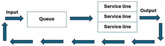
Figure 6.
Closed queueing service system.
Monte Carlo is a class of algorithms for the stochastic simulation of systems. The method relies on the random generation of pseudorandom numbers. It is commonly used for the evaluation of integral, especially multidimensional, systems, where conventional methods fail or are inefficient. The Monte Carlo method also has wide applicability for solving differential equations. For modeling random processes in construction activities, the Monte Carlo method appears to be the most suitable regarding both speed and the quality of results. The underlying idea is simple: given random draws, one estimates the expected value of a quantity that results from a random process. Implementing a computational model of such a process is relatively straightforward today, and after performing enough simulations, the data can be processed using classical statistical methods to obtain the mean and the standard deviation [13,45].
The Monte Carlo method requires constructing a model of a real system that possesses the same probabilistic characteristics as that system (randomness is induced via random numbers). The model must then be refined using various coefficients and stochastic influences that affect the entire system. The experimenter can subsequently analyze the model repeatedly and iteratively calibrate its behavior.
When generating random values in a Monte Carlo simulation, one must employ an appropriate probability distribution. The developed system allows the user to specify the type of distribution either from predefined options (normal, exponential, gamma, Erlang) or from user-defined types.
By combining the Monte Carlo method with queueing theory, several alternative solutions are obtained that satisfy the specified task. For each alternative, the optimization parameters are computed. The synthetic data generated in this way is then used in the subsequent step for training the AI model.
The last two steps of modeling (the development of the AI model and the implementation of the developed model into the real environment) are not the subject of the present study; they only outline the subsequent procedure for system development and the application of the generated synthetic data. The following section will provide a detailed description of the functionality of the developed model for the generation of synthetic data for the AI model aimed at optimizing construction machine configurations.
3. Generation of Synthetic Data for Model Optimization
The following section provides a detailed step-by-step description of the workflow for generating synthetic data for the model designed to optimize machine configurations, with a specific focus on earthworks in construction. An example of a simulation calculation using queueing theory is provided in Appendix A. The source code of the generator (written in PHP version 8.2.15 as web application [49]) is available in a publicly accessible repository [50]. The data are stored in a MySQL (MariaDB version 5.5.68) database, and the database structure is made available in a publicly accessible repository in SQL format [50].
Figure 7 presents a block diagram illustrating the fundamental steps involved in synthetic data generation, including the key components of the Data Governance Policy.
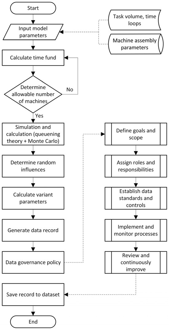
Figure 7.
The fundamental steps in synthetic data generation.
The real large-scale construction project CTU—New Building Device (NBD) was selected as a case study to demonstrate the sample simulation of the synthetic data presented in this manuscript. Based on the project’s bill of quantities, the total task volume reached 3350 m3 (7537 t). The excavation and transport processes were modeled for a large construction site using various machine assemblies. This case study offers a step-by-step simulation of the generated synthetic data, which is further verified in Section 4.
For the necessary functionality, it is essential to introduce input parameters into the system that describe both the contractual project and the characteristics of the construction site and construction machinery, including stochastic and optimization coefficients:
- Task parameters: Task volume, start and completion dates, maximum available working area, shift length, variable costs, and machine productivity coefficients according to project complexity.
- Machine parameters (machine catalog): Average machine performance, average cycle time, maximum available number of units, minimum working area, variable cost, fixed cost, probability of failure, mean time to repair, average cost of failure removal, energy consumption, and CO2 emissions.
- Kendall’s classification of queueing systems (X/Y/c) for data generation [51].
- Stochastic parameters: Randomness of failures, randomness of weather conditions, randomness of traffic complications, randomness of emergency states, and randomness of human factors.
An example of synthetic data generation is presented in Table 1. The number of synthetic data records is calculated according to the following formula and is limited by the computational performance available for the generation of the synthetic data:
where is the number of admissible variants of served machines, is the number of admissible variants of serving machines, and is the number of task variants to be completed by the production factor.

Table 1.
An example of synthetic data generation for 25,000 process input cycles.
The volume of synthetic data can reach hundreds of millions of records, and for each variant, a stochastic simulation of construction processes is performed based on repeated execution of work cycles. Data synthesis may therefore require significant computational capacity. A training dataset generated for testing purposes contained 17,280,000 records [50]. The individual simulation results according to variant 6 (Table 1) are presented in Table 2 and Figure 8.
Table 2.
The simulation and computation for variant 6: Caterpillar 300.9D (2 units)/Tatra 163 (20 units).
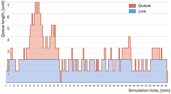
Figure 8.
Simulation of queue length and service time.
Figure 8 presents a graphical representation of the simulation for the first 200 ticks in the scenario with two service lines. Each tick corresponds to one minute of simulation time. During each tick, a customer may enter the system. If service lines are available, the service process begins (blue area). Upon completion of service, the customer leaves the queue, releases the service line, and performs a work cycle, after which they rejoin the end of the queue. If all service lines are occupied, the customer joins the queue and waits until a line becomes available (red area). Table 1 presents the average time values for the complete simulation (25,000 process input cycles). The total task completion time is calculated as: (Average Input Time + Average Waiting Time) × Number of process input cycles = Total Time task completion. The parameters of the simulated queue are also calculated, including the Average Waiting Time in the queue, as well as the Average and Maximum Queue length. Table 2 illustrates the status of the service lines and the queue during each tick of the simulation.
The resulting simulation record contains the calculated optimization parameters (Table 3). The table summarizes the performance of different equipment configurations in terms of total cost, completion time, CO2 emissions, fuel consumption, and the number of failures. Each scenario represents a distinct combination of serving and served units, reflecting variations in machine allocation. The results indicate that configurations with a higher number of serving units tend to reduce completion time and emissions, while also maintaining a lower number of failures. However, this improvement is often accompanied by a moderate increase in total cost, highlighting the trade-off between efficiency and operational expenses.
Table 3.
The calculated optimization parameters.
4. Verification and Validation of Synthetic Data
Every theoretical insight must be verified in practice. A theory or scientific research gains value only when it can be applied in the real world. The functionality of the developed synthetic data generator for subsequent training of the AI model, aiming to optimize construction machine configurations, was verified on a real large-scale construction project: CTU—New Building Device (NBD).
Verification was carried out during the construction stage “Site Preparation” for the processes “Loading of topsoil and subsoil and transport to landfill within 20 km”, “Loading and transport of demolished asphalt materials for recycling within 20 km”, and “Loading and transport of demolished materials to an intermediate landfill within 20 km”. According to the bill of quantities, the task volume was 3350 m3 or 7537 t.
The primary real-world measurements were conducted using the provided time-lapse recording (Figure 9). The time-lapse was carried out with two cameras placed outside the construction site [33]. These data served as a reference for comparing the synthetic data with the actual execution of construction work.
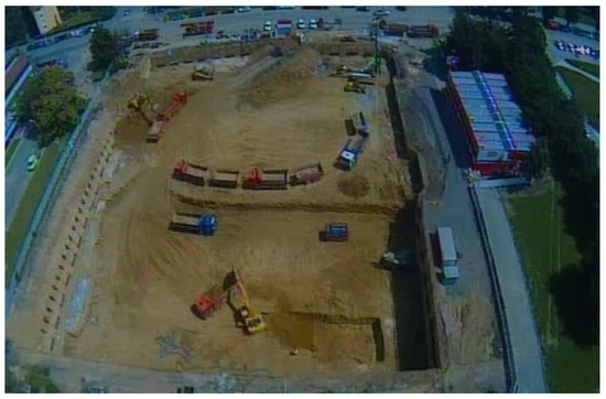
Figure 9.
Time-lapse recording from a camera (CTU–New Building Device).
To increase the reliability of verification and validation, an additional 10 construction projects were analyzed, carried out between 2020 and 2025 in the Czech Republic. These were anonymized projects of residential and civil construction. The aggregated comparative data, including parameter deviations, are presented in Table 4. The overall deviation was calculated as a weighted average of the individual deviations, assuming equal parameter weights. The overall deviation of actual data from synthetic data for the 10 projects analyzed did not exceed 13%.
Table 4.
The aggregated comparative data (synthetic/real).
The quality of data is particularly crucial when it comes to synthetic data. The validation process assesses the data’s accuracy, consistency, realism, and utility to ensure it is genuinely suitable for the intended task. This process helps mitigate the risks associated with synthetic data that has not undergone rigorous testing. Table 5 presents the final statistical evaluation of the synthetic dataset in comparison with the real dataset, conducted across ten projects and forty-nine independent construction tasks. The analysis employed correlation analysis (R2, Pearson correlation), comparison of key statistical indicators Root Mean Square Error (RMSE), as well as the F-test and the Kolmogorov–Smirnov test to assess the normality of the data distribution. A comprehensive report detailing the statistical evaluation of synthetic data quality is provided in ref. [52].
Table 5.
Summary of Model Performance Metrics.
The model demonstrates very high accuracy for Total Cost (R2 = 0.96), CO2 Emissions (R2 = 0.93), Fuel Consumption (R2 = 0.90), and Completion Time (R2 = 0.87). In contrast, the Number of Failures metric shows poor performance, with a low R2 value (R2 = 0.15) indicating that the model explains only a small fraction of its variance. The RMSE values for the first four metrics are reasonable relative to their respective scales, whereas the RMSE for Failures (RMSE = 1.70) suggests higher relative errors. The synthetic and observed values exhibit strong positive Pearson correlations for all metrics except Number of Failures (correlation = 0.38), confirming poor linear agreement in that case. Statistical validation further supports these findings. For Total Cost, Completion Time, CO2 Emissions, and Fuel Consumption, F < Fcrit, indicating that the model’s regression results are statistically significant and valid. Conversely, for Number of Failures, F > Fcrit, showing that predictions are not statistically significant. The Kolmogorov–Smirnov test confirms that residuals for the first four metrics satisfy normality assumptions (K–S < K–Scrit), whereas for Number of Failures, K–S > K–Scrit, implying that residuals deviate from normality and thus reduce model reliability for this variable. Figure 10 presents a graphical representation of the Kolmogorov–Smirnov statistical test for the following metrics: Total Cost, Completion Time, Fuel Consumption, and CO2 Emissions.
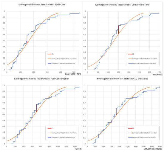
Figure 10.
Kolmogorov–Smirnov statistical test.
5. Conclusions
Summary of main results: This study introduces a novel methodology for generating synthetic data to train optimization models for construction machinery assemblies. The approach combines queuing theory and Monte Carlo simulation to produce realistic, large-scale datasets efficiently. The developed model and generator, validated against real construction data, provide a practical and scalable solution that reduces data collection costs and supports improved design and performance of construction machinery in earthworks. The generator enables large-scale simulation and data generation for AI model training aimed at optimizing construction machine configurations. The system demonstrated the following:
- High computational efficiency that is capable of generating tens of millions of records.
- The implementation of queueing theory and Monte Carlo simulations to model stochastic construction processes.
- Practical verification on 10 real construction projects, where the maximum deviation between synthetic and real data did not exceed 13%.
- Each large-scale project comprises between three and seven independent construction tasks. For each task, real-world data were independently collected and evaluated. In total, 49 comparisons were conducted, and the outcomes were aggregated and synthesized into ten consolidated project-level records.
- Based on statistical verification using correlation analysis (R2, Pearson correlation), comparison of key statistical indicators (RMSE, F-test), and the Kolmogorov–Smirnov test, the generated synthetic data demonstrate good model performance for Total Cost (R2 = 0.96), CO2 Emissions (0.93), Fuel Consumption (0.90), and Completion Time (0.87). However, the model shows poor performance for the Number of Failures, as indicated by a low R2 value, weak correlation, lack of statistical significance, and non-normal residuals.
6. Discussion
6.1. Limitations
While the results are promising, the present study represents only an initial step in developing specialized optimization software. Several limitations have been identified:
- The mathematical model relies on simplifications that may not fully capture the complexity of real construction processes.
- Verification has so far been limited to 10 construction projects (49 tasks), restricting the generalizability of the findings.
- The current set of optimization indicators, while comprehensive, may not fully cover all relevant factors in diverse construction contexts.
- The generator does not incorporate an economic model that accounts for the marginal cost associated with each additional resource. Consequently, the model operates without estimating these marginal costs, which does not fully represent real-world conditions and could be improved in future work.
6.2. Future Directions
Further research is required to extend and validate the model:
- Refining the mathematical framework to better approximate actual technological processes and improve generation ability for metric Number of Failure.
- Expanding verification to a broader set of construction projects to demonstrate universality and robustness.
- Incorporating additional optimization criteria, including advanced environmental indicators and safety parameters.
- Validate the model results through cross-national comparisons to enhance external validity.
- Validate the model results through model-based testing (utility testing) and expert review.
- Examine and compare alternative algorithms for generating synthetic data in construction processes (e.g., Markov chains).
6.3. Implications and Significance
Although the developed system is not yet perfect, it carries significant potential for practical application. Its real-world deployment is expected to refine and improve the mathematical model further, making it a valuable tool for both operational and strategic planning in construction management. By simplifying AI model training and enabling optimization of mechanized processes, the generator can help reduce costs, shorten construction times, and mitigate environmental impacts in the construction industry. Beyond cost reduction and efficiency gains, the model also has implications for urban land-use efficiency, tax policy, and sustainable development. When applied to public or urban construction, its optimization outcomes could influence land valuation, zoning density, and regional tax revenues, thereby affecting local fiscal planning. Integrating such data-driven optimization into urban policy frameworks can thus enhance not only construction performance but also the institutional and sustainability dimensions of urban growth. More efficient construction cycles and resource utilization can also lead to a more adaptive and sustainable urban form, consistent with the goals of the EU Green Deal and sustainable urban mobility frameworks.
6.4. Legal and Ethical Positioning of Synthetic Data
The dataset utilized in this paper comprises exclusively synthetic data, rigorously validated against anonymized and non-sensitive reference sources. This methodological approach ensures that no information can be re-associated with any identifiable natural or legal person. All machine assembly registration identifiers, corporate logos, and proprietary symbols were systematically removed during the data preprocessing and sanitization phase. In accordance with the General Data Protection Regulation (GDPR, Regulation (EU) 2016/679), such data are considered to fall outside the regulatory scope of personal data processing, provided that the anonymization process is irreversible and the probability of re-identification remains negligible (Recital 26, GDPR). Nonetheless, a residual risk of re-identification cannot be entirely excluded, particularly if the synthetic data generation process closely reproduces statistical patterns inherent to the original dataset. To mitigate this potential risk, controlled parameterization of the generative model and systematic post-generation validation procedure was implemented. These measures were designed to minimize model overfitting and prevent the inadvertent disclosure or reconstruction of original data distributions.
The EU Artificial Intelligence Act (Regulation (EU) 2024/1689) underscores the critical importance of robust data governance, transparency, and accountability in artificial intelligence systems, even in contexts where no personal data are directly processed. In accordance with these principles, the present paper emphasizes the traceability and reproducibility of the synthetic data generation pipeline. While the question of data ownership is comparatively attenuated in the case of synthetic datasets—since no original data subjects can assert rights over generated samples, the issues of algorithmic bias and model accountability remain of paramount significance. Consequently, the proposed approach incorporates quantitative bias assessment metrics and model explainability mechanisms, thereby advancing responsible AI development in alignment with the EU’s risk-based regulatory framework.
Funding
This research was funded by the Czech Technical University in Prague, Faculty of Civil Engineering, Student Grant Competition, under grant number SGS23/148/OHK1/3T/11, Increasing the sustainability of masonry and concrete structures using robots, and grant number SGS25/115/OHK1/3T/11, Technological procedures for treatment and processing of deposited CCP products containing primary and secondary gypsum.
Data Availability Statement
Conflicts of Interest
The author declares that there are no competing financial, professional, or personal interest from other parties.
Abbreviations
The following abbreviations are used in this manuscript:
| AI | Artificial intelligence |
| MRTS | Marginal rate of technical substitution |
| MP | Marginal product |
| PHP | Personal home page |
| FIFO | FIFO principle (first in–first out) |
| RMSE | Root mean square error |
| F-test | Fisher’s test of variance |
| K–S test | Kolmogorov–Smirnov test |
| R2 | Coefficient of determination |
| CO2 | Carbon dioxide |
| GDPR | General Data Protection Regulation |
Appendix A
This appendix contains the results of the simulation and the calculation of a construction machine configuration using queueing theory.
The input parameters of the mathematical model:
- Construction process: Excavation works and foundation pit.
- The total soil volume is therefore calculated as follows:
Truck (dumper) parameters are presented in Table A1, based on [54]. A dumper with a loading capacity of 15 m3 is considered. The average round-trip time from the construction site to the disposal area is 40 min. The financial costs of machine operation include fixed costs of CZK 3000 and variable costs of 1000 CZK per hour. The maximum number of available dumpers is 15. The probability of failure is 2% per day, with an average repair time of 2 h [54]. The service connection time to the excavator is 2 min.
Table A1.
The input parameters for the truck.
Table A1.
The input parameters for the truck.
| Parameter | Value |
|---|---|
| Load capacity, m3 | 15 |
| Average travel time (travel loop 25 km), min | 40 |
| Average unloading time, min | 2 |
| Average loading time, min | 15 60/P |
| Fixed costs, CZK | 3000 |
| Variable costs, CZK/hour | 1000 |
| Probability of failure, %/day | 2 |
| Average repair time, min | 60 |
| Maximum number of dumpers | 15 |
A work shift is h per day, 40 h per week. The time limit for the construction task is a maximum of 2 weeks ( working hours, i.e., 4800 min). The basic time unit is the minute.
Excavator input parameters are given in Table A2, based on [54]. Most parameters are either specified by the manufacturer or estimated based on field observation and monitoring. The required hourly performance of the excavator, excluding random failures, is calculated as follows:
Table A2.
The input parameters of the excavator.
Table A2.
The input parameters of the excavator.
| Parameter | Value |
|---|---|
| Bucket capacity, m3 | 2 |
| Average cycle time, min | 0.83 |
| Average productivity , m3/h | 100 |
| Fixed costs, CZK | 5000 |
| Variable costs, CZK/hour | 2000 |
| Probability of failure, %/day | 2 |
| Average repair time, min | 60 |
The average cycle time of the dumper without random factors is calculated as follows:
The hourly productivity of the dumper is calculated as follows:
The minimum number of dumpers required to fully utilize the excavator, ignoring random factors, is calculated as follows:
Further calculations concerning stochastic influences are performed within the simulation software. After incorporating random variables (machine failures) into the mathematical model, simulations indicate an extension of service times :
The intervals between service entries are likewise extended:
The average dumper cycle time including failures is calculated as follows:
This computation is summarized in Table A3. The service cycles of excavators and dumpers are interdependent at the loading point. Due to random inter-arrival intervals of dumpers, queues inevitably form. Therefore, queuing theory is suitable for analyzing the interaction between the transport system and the excavator.
For optimal machine fleet design, further parameters of queuing theory are required:
- Service intensity:
- Arrival intensity:
- System load factor:
The queuing calculations in Table A3 demonstrate that processing an excavation volume of m3 within 80 working hours (4800 min) requires 11 dumpers ().
Table A3.
The queuing calculations for processing an excavation volume.
Table A3.
The queuing calculations for processing an excavation volume.
| n | ρ | S (n·ρ) | V | L | M | I | N | TF [min] | TC [min] | T [min] | Q [m3] |
|---|---|---|---|---|---|---|---|---|---|---|---|
| 1 | 0.1440 | 1.144 | 0.8740 | 0.8740 | 0.1259 | 0.1259 | 0.0000 | 0.0000 | 48.11 | 36,083 | 998 |
| 2 | 0.2881 | 1.3296 | 0.8604 | 1.7208 | 0.2791 | 0.2479 | 0.0312 | 0.7628 | 48.87 | 18,327 | 1964 |
| 3 | 0.4321 | 1.5746 | 0.8444 | 2.5332 | 0.4667 | 0.3649 | 0.1018 | 1.6909 | 49.80 | 12,450 | 2892 |
| 4 | 0.5762 | 1.9073 | 0.8255 | 3.3022 | 0.6977 | 0.4757 | 0.2220 | 2.8278 | 50.94 | 9551 | 3769 |
| 5 | 0.7202 | 2.3738 | 0.8034 | 4.0174 | 0.9825 | 0.5787 | 0.4038 | 4.2271 | 52.34 | 7851 | 4586 |
| 6 | 0.8643 | 3.0518 | 0.7778 | 4.6670 | 1.3329 | 0.6723 | 0.6606 | 5.9525 | 54.06 | 6758 | 5327 |
| 7 | 1.0084 | 4.0775 | 0.7484 | 5.2391 | 1.7608 | 0.7547 | 1.0060 | 8.0750 | 56.19 | 6020 | 5980 |
| 8 | 1.1524 | 5.6993 | 0.7154 | 5.7235 | 2.2764 | 0.8245 | 1.4518 | 10.667 | 58.78 | 5510 | 6533 |
| 9 | 1.2965 | 8.3893 | 0.6793 | 6.1141 | 2.8858 | 0.8808 | 2.0050 | 13.790 | 61.90 | 5158 | 6979 |
| 10 | 1.4405 | 13.085 | 0.6411 | 6.4110 | 3.5889 | 0.9235 | 2.6653 | 17.482 | 65.59 | 4919 | 7318 |
| 11 | 1.5846 | 21.736 | 0.6020 | 6.6222 | 4.3777 | 0.9539 | 3.4237 | 21.741 | 69.85 | 4763 | 7559 |
| 12 | 1.7287 | 38.575 | 0.5634 | 6.7616 | 5.2383 | 0.9740 | 4.2643 | 26.520 | 74.63 | 4664 | 7718 |
| 13 | 1.8727 | 73.244 | 0.5266 | 6.8467 | 6.1532 | 0.9863 | 5.1668 | 31.734 | 79.84 | 4606 | 7815 |
| 14 | 2.0168 | 148.72 | 0.4924 | 6.8948 | 7.1051 | 0.9932 | 6.1118 | 37.276 | 85.39 | 4574 | 7870 |
| 15 | 2.1608 | 322.37 | 0.4613 | 6.9200 | 8.0799 | 0.9968 | 7.0830 | 43.042 | 91.15 | 4558 | 7899 |
Table A3 describes queueing system performance metrics. Column n represents the number of parallel links (e.g., machines or operators). n·ρ indicates the total system load factor (utilization), showing the overall load on all links combined. S (n·ρ) is a performance or efficiency factor reflecting how system effectiveness changes with increasing utilization. V denotes the service efficiency, or the proportion of time servers are actively working. L is the average number of entities (such as trucks or tasks) present in the system, while M represents the average number currently being serviced. I shows the average number of idle servers, and N is the average queue length, i.e., the number of entities waiting for service. TF [min] refers to the total flow time, the average time an entity spends in the system including both waiting and service. TC [min] is the cycle time per entity, representing one complete operational cycle (e.g., travel, load, unload, and wait). T [min] indicates the average service time for a single operation, and Q [m3] is the total processed or transported volume in cubic meters corresponding to the configuration.
The initial cycle increases due to queueing delays and continues to extend overtime. The performance of the transport system does not grow linearly with the number of dumpers (see Figure A1).

Figure A1.
The performance of the transport system.
Finally, the financial cost analysis is performed. The optimal configuration corresponds to the solution with the lowest total costs.
Appendix B
This appendix contains the pseudocode of the simplified synthetic data generator for the optimization of construction machine assemblies. The functions implementing the queuing theory–based simulation, the computation of economic parameters for the variants, and the incorporation of stochastic effects are presented solely in an input/output format. The detailed implementations of these functions are provided in ref. [50]; each comprises several hundred lines of source code, which are not practical to represent in pseudocode form.
| START 1. IMPORTS import table/CSV library (e.g. pandas) 2. LOAD INPUT DATA task_table ← read CSV “data_input/task.csv” machines_table ← read CSV “data_input/machine.csv” 3. BUILD MACHINE VARIANTS //customer/transport machines: SET customer_table ← filter machines_table where group == customer //operator/loading machines: SET operator_table ← filter machines_table where group1 == operator 4. SIMULATION PARAMETERS SET task_bins, volume_min, volume_max SET travel_bins, travel_min, travel_max SET operator_min, operator_max SET customer_min, customer_max //count of total number of variants COMPUTE total_variants ← travel_bins * task_bins * (operator_max − operator_min + 1) * (customer_max − customer_min + 1) * ROW_COUNT(operator_table) * ROW_COUNT(customer_table) 5. PREPARE OUTPUT HEADER SET columns ← [“model”, “volume”, “travel_time”, “lambda”, “mu”, “rho”, “operator_id”, “operator_count”, “customer_id”, “customer_count”, “input_count”, “input_time”, “service_time”, “waiting_time”, “queue_avg”, “queue_max”, “total_time”, “total_cost”, “total_co2”, “total_fuel”, “total_failure”] OPEN CSV file “data_output/synthetic_data.csv” FOR writing WRITE columns AS first line (comma-separated) 6. MAIN GENERATION LOOP SET record_counter, default_model_id, default_unload_time_s FOR EACH operator_row IN operator_table: //extract machine parameters SET operator_db_id ← operator_row[“id”] SET operator_productivity ← operator_row[“work_output_unit_h”] SET operator_bucket ← operator_row[“units_count”] SET operator_cycle_sec ← operator_row[“work_cycle_sec”] SET operator_price_usd ← operator_row[“machine_price_usd”] //extract economic parameters FC—Fixed Cost, VC—Variable Cost SET operator_FC ← operator_row[“machine_FC”] SET operator_VC ← operator_row[“machine_VC”] //extract technical parameters Failure, Fuel consumption, CO2 production SET operator_failure_rate ← operator_row[“machine_ failure_rate”] SET operator_repair_rate ← operator_row[“machine_ failure_repair”] SET operator_fuel_h ← operator_row[“machine_ failure_fuel_h”] SET operator_co2_h ← operator_row[“machine_ failure_ co2_h”] END FOR FOR EACH customer_row IN customer_table: //extract machine parameters SET customer_db_id ← customer_row[“id”] SET customer_productivity ← customer_row[“work_output_unit_h”] SET customer_bucket ← customer_row[“units_count”] SET customer_cycle_sec ← customer_row[“work_cycle_sec”] SET customer_price_usd ← customer_row[“machine_price_usd”] //extract economic parameters FC—Fixed Cost, VC—Variable Cost SET customer_FC ← customer_row[“machine_FC”] SET customer_VC ← customer_row[“machine_VC”] //extract technical parameters Failure, Fuel consumption, CO2 production SET customer_failure_rate ← customer_row[“machine_ failure_rate”] SET customer_repair_rate ← customer_row[“machine_ failure_repair”] SET customer_fuel_h ← customer_row[“machine_ failure_fuel_h”] SET customer_co2_h ← customer_row[“machine_ failure_ co2_h”] END FOR //iterate over task volumes SET volume_step ← (volume_max − volume_min)/(task_bins − 1) FOR volume FROM volume_min TO volume_max STEP volume_step: //number of transport cycles needed to reach this volume SET input_count ← FLOOR( volume/load_capacity ) //iterate over travel times SET travel_step ← (travel_max − travel_min)/(travel_bins − 1) FOR travel_time FROM travel_min TO travel_max STEP travel_step: //iterate over operator fleet size FOR operator_count FROM operator_min TO operator_max: //iterate over customer fleet size FOR customer_count FROM customer_min TO customer_max: //Service intensity (mu): //how fast the “service” can process arriving loads SET mu ← (customer_bucket * 60)/operator_productivity //Arrival intensity (lambda): //arrivals are limited by transport + unload time SET lambda ← 1/(unload_time + travel_time) //System load factor SET rho ← lambda/mu //build output row (same order as columns) SET total_time = FUNCTION_TIME(row) SET total_cost = FUNCTION_COST(row) SET total_fuel = FUNCTION_FUEL(row) SET total_co2 = FUNCTION_CO2(row) SET total_failure = FUNCTION_FAILURE(row) SET row ← [default_model_id, volume, travel_time, lambda, mu, rho, operator_row_index, operator_count customer_row_index, customer_count, input_count, total_time, total_cost, total_fuel, total_co2, total_failure] WRITE row TO CSV END FOR END FOR END FOR END FOR 7. OPTIONAL POSTPROCESS //Data Governance Policy FUNCTION_DATA_GOVERNANCE(all row) END PROGRAM |
References
- OECD. OECD Compendium of Productivity Indicators 2025; OECD Publishing: Paris, France, 2025. [Google Scholar] [CrossRef]
- World Economic Forum. Shaping the Future of Construction: A Breakthrough in Mindset and Technology; World Economic Forum: Geneva, Switzerland, 2016; Available online: https://www3.weforum.org/docs/WEF_Shaping_the_Future_of_Construction_full_report__.pdf (accessed on 10 November 2025).
- Pal, U.K.; Zhang, C.; Haupt, T.C.; Li, H.; Su, L. The Evolution of Construction 5.0: Challenges and Opportunities for the Construction Industry. Buildings 2024, 14, 4010. [Google Scholar] [CrossRef]
- Samuelson, O.; Stehn, L. Digital Transformation in Construction—A Review. J. Inf. Technol. Constr. 2023, 28, 385–404. [Google Scholar] [CrossRef]
- McKinsey Global Institute. Reinventing Construction: A Route to Higher Productivity. February 2017. Available online: https://www.mckinsey.com/capabilities/operations/our-insights/reinventing-construction-through-a-productivity-revolution (accessed on 10 November 2025).
- Emmanuella, O.N.; Tari, Y.E.; Kingsley, O.O. The Importance of Interdisciplinary Collaboration for Successful Engineering Project Completions: A Strategic Framework. World J. Eng. Technol. Res. 2023, 2, 001–016. [Google Scholar] [CrossRef]
- You, Z.; Wu, C. A Framework for Data-Driven Informatization of the Construction Company. Adv. Eng. Inform. 2019, 39, 269–277. [Google Scholar] [CrossRef]
- Gumusburun Ayalp, G.; Arslan, F. Modeling Critical Rework Factors in the Construction Industry: Insights and Solutions. Buildings 2025, 15, 606. [Google Scholar] [CrossRef]
- RazaviAlavi, S.; AbouRizk, S. Site Layout and Construction Plan Optimization Using an Integrated Genetic Algorithm Simulation Framework. J. Comput. Civ. Eng. 2017, 31, 04017011. [Google Scholar] [CrossRef]
- Bahadori-Jahromi, A.; Room, S.; Paknahad, C.; Altekreeti, M.; Tariq, Z.; Tahayori, H. The Role of Artificial Intelligence and Machine Learning in Advancing Civil Engineering: A Comprehensive Review. Appl. Sci. 2025, 15, 10499. [Google Scholar] [CrossRef]
- Fabian, F.; Kluiber, Z. The Monte Carlo Method and Its Potential Applications/Metoda Monte Carlo a Možnosti Jejího Uplatnění, 1st ed.; Prospektrum: Prague, Czech Republic, 1998; ISBN 80-7175-058-1. [Google Scholar]
- Kendall, D.G. Stochastic Processes Occurring in the Theory of Queues and Their Analysis by the Method of the Imbedded Markov Chain. Ann. Math. Statist. 1953, 24, 338–354. [Google Scholar] [CrossRef]
- Hastings, W.K. Monte Carlo Sampling Methods Using Markov Chains and Their Applications. Biometrika 1970, 57, 97–109. [Google Scholar] [CrossRef]
- Luenberger, D.G. Linear and Nonlinear Programming, 2nd ed.; Addison-Wesley: Reading, MA, USA, 1996; ISBN 978-0201157949. [Google Scholar]
- Ackoff, R.L.; Sasieni, M.W. Fundamentals of Operations Research; John Wiley: London, UK, 1970; ISBN 978-0471003335. [Google Scholar]
- Jarský, Č. Towards a Mathematical Model of Construction Processes. Ph.D. Thesis, CTU in Prague, Prague, Czech Republic, 1981. [Google Scholar]
- Jarský, Č. Automation in the Planning and Management of Construction Projects, 1st ed.; CONTEC: Kralupy nad Vltavou, Czech Republic, 2000; ISBN 80-238-5384-8. [Google Scholar]
- Motyčka, V.; Gašparík, J.; Přibyl, O.; Štěrba, M.; Hořínková, D.; Kantová, R. Effective Use of Tower Cranes over Time in the Selected Construction Process. Buildings 2022, 12, 436. [Google Scholar] [CrossRef]
- Břoušek, M.; Vávra, I.; Zapletal, I. Civil Engineering Structures—Technology; Alfa Konti: Bratislava, Slovakia, 1995; ISBN 80-88739-14-4. [Google Scholar]
- Tažiková, A.; Struková, Z.; Kozlovská, M. An Analysis of Real Site Operation Time in Construction of Residential Buildings in Slovakia. Sustainability 2023, 15, 1529. [Google Scholar] [CrossRef]
- Puchov, G.; Chatiashvili, C. Models of Technological Processes; Technika: Moscow, Russia, 1974. [Google Scholar]
- Pontrjagin, L. Mathematical Theory of Optimal Processes; Nauka: Moscow, Russia, 1983. [Google Scholar]
- Zavadskas, E. Comprehensive Evaluation and Selection of Resource-Efficient Decisions in Construction; Mokslas: Vilnus, Lithuania, 1987. [Google Scholar]
- Jarský, Č.; Popenková, M.; Gašparík, J.; Šťastný, P. On Use of Construction Technology Designs for Expert Opinions. Sustainability 2022, 14, 5672. [Google Scholar] [CrossRef]
- Berezneva, T.; Grosmann, C. Application of Operations Research in Economics; Ekonomika: Moscow, Russia, 1977. [Google Scholar]
- Ignatjev, I.; Iljevskij, B. Modelling of Machine Systems; Mashinostroenie: Leningrad, Russia, 1986. [Google Scholar]
- Zavadskas, E. Systematic Evaluation of Construction Production Decisions; Stroizdat: Leningrad, Russia, 1991; ISBN 5-274-01169-1. [Google Scholar]
- Pervozvanskij, A. Mathematical Models in Production Management; Nauka: Moscow, Russia, 1975. [Google Scholar]
- Bakaev, A. Mathematical Methods in Planning; Naukova Dumka: Kiev, Ukraine, 1968. [Google Scholar]
- Motyčka, V. Optimization of the Tower Cranes Planning: Contribution to the Modelling of the Construction Site Production Area; VUTIUM: Brno, Czech Republic, 2007; ISBN 978-80-214-3400-4. [Google Scholar]
- Jarsky, C. On Mathematical Stochastic Modelling and Optimization of Construction Processes; Akadémiai Kiadó: Budapest, Hungary, 1984. [Google Scholar]
- Raghunathan, T.E. Synthetic Data. Annu. Rev. Stat. Appl. 2021, 8, 129–140. [Google Scholar] [CrossRef]
- Usmanov, V. On Mathematical Modeling and Optimization of Construction Processes. Ph.D. Thesis, CTU in Prague, Prague, Czech Republic, 2016. [Google Scholar]
- Hopocký, A.; Makýš, P.; Ďubek, M. Computational Basis of Completed Works for the Quantities of Budget Items. Czech J. Civ. Eng. 2024, 10, 84–90. [Google Scholar] [CrossRef]
- Kim, K.-M.; Kwak, J.W. PVS-GEN: Systematic Approach for Universal Synthetic Data Generation Involving Parameterization, Verification, and Segmentation. Sensors 2024, 24, 266. [Google Scholar] [CrossRef]
- Tsitsiashvili, G. Construction and Analysis of Queuing and Reliability Models Using Random Graphs. Mathematics 2021, 9, 2511. [Google Scholar] [CrossRef]
- Ebid, A.M.; Ammar, T.; Mahdi, I.; Hegazy, H. Evaluating the Planning Efficiency for Repetitive Construction Projects Using Monte Carlo Simulation Technique. Sci. Rep. 2025, 15, 27520. [Google Scholar] [CrossRef] [PubMed]
- Mostofi, F.; Behzat Tokdemir, O.; Toğan, V. Generating Synthetic Data with Variational Autoencoder to Address Class Imbalance of Graph Attention Network Prediction Model for Construction Management. Adv. Eng. Inform. 2024, 62, 102606. [Google Scholar] [CrossRef]
- Schuster, A.; Hagmanns, R.; Sonji, I.; Löcklin, A.; Petereit, J.; Ebert, C.; Weyrich, M. Synthetic Data Generation for the Con-tinuous Development and Testing of Autonomous Construction Machinery. Automatisierungstechnik 2023, 71, 953–968. [Google Scholar] [CrossRef]
- Xu, L.; Liu, H.; Xiao, B.; Luo, X.; Zhu, Z. Synthetic Simulated Data for Construction Automation: A Review. In Construction Research Congress 2024; American Society of Civil Engineers: Des Moines, IA, USA, 2024; pp. 527–536. [Google Scholar] [CrossRef]
- Zhang, H.; Yu, L. Site Layout Planning for Prefabricated Components Subject to Dynamic and Interactive Constraints. Autom. Constr. 2021, 126, 103693. [Google Scholar] [CrossRef]
- Kim, J.; Wang, I.; Yu, J. Experimental Study on Using Synthetic Images as a Portion of Training Dataset for Object Recognition in Construction Site. Buildings 2024, 14, 1454. [Google Scholar] [CrossRef]
- Neuhausen, M.; Herbers, P.; König, M. Using Synthetic Data to Improve and Evaluate the Tracking Performance of Construction Workers on Site. Appl. Sci. 2020, 10, 4948. [Google Scholar] [CrossRef]
- Sokolowski, J.A.; Banks, C.M. Modeling and Simulation Fundamentals: Theoretical Underpinnings and Practical Domains; Wiley: Hoboken, NJ, USA, 2010; ISBN 978-0-470-48674-0. [Google Scholar]
- Klvaňa, J. Modelling 20, 3rd ed.; Vydavatelství ČVUT: Prague, Czech Republic, 2005; ISBN 80-01-03263-9. [Google Scholar]
- Soukupová, J. Microeconomics, 3rd ed.; Management Press: Prague, Czech Republic, 2002; ISBN 80-7261-061-9. [Google Scholar]
- Jarský, Č. Construction Technology II: Preparation and Execution of Construction Projects; Akademické Nakladatelství CERM: Brno, Czech Republic, 2019; ISBN 978-80-7204-994-3. [Google Scholar]
- Rektorys, K. Overview of Applied Mathematics, 7th ed.; Prometheus: Prague, Czech Republic, 2000. [Google Scholar]
- PHP Documentation. Available online: https://www.php.net/download-docs.php (accessed on 13 October 2025).
- Synthetic Data Generation for AI-Driven Optimization of Construction Machinery Assemblies. Available online: https://github.com/UsmanovSla/GeneratorSyntheticData (accessed on 13 October 2025).
- Rovetto, C.; Cruz, E.; Nuñez, I.; Santana, K.; Smolarz, A.; Rangel, J.; Cano, E.E. Minimizing Intersection Waiting Time: Proposal of a Queue Network Model Using Kendall’s Notation in Panama City. Appl. Sci. 2023, 13, 10030. [Google Scholar] [CrossRef]
- Summary of Model Performance Metrics. Available online: http://www.robostav.cz/download/data/GeneratorSyntheticData_Validation.pdf (accessed on 4 November 2025).
- Czech Technical Standard 73 3050; Earth Works. General Requirements. Czech Standards Institute: Prague, Czech Republic, 1999.
- Komatsu: Manufacturer of Construction, Mining, Forestry, and Industrial Heavy Equipment. Available online: https://www.komatsu.com/en-us (accessed on 17 October 2025).
Disclaimer/Publisher’s Note: The statements, opinions and data contained in all publications are solely those of the individual author(s) and contributor(s) and not of MDPI and/or the editor(s). MDPI and/or the editor(s) disclaim responsibility for any injury to people or property resulting from any ideas, methods, instructions or products referred to in the content. |
© 2025 by the author. Licensee MDPI, Basel, Switzerland. This article is an open access article distributed under the terms and conditions of the Creative Commons Attribution (CC BY) license (https://creativecommons.org/licenses/by/4.0/).