Article

Statistical Analysis of Factors Influencing Segmental Joint Opening in a Soft Soil Tunnel

1
Qingdao Metro Line 8 Co., Ltd., Qingdao 266000, China
2
College of Civil Engineering, Henan University of Technology, Zhengzhou 450001, China
*
Author to whom correspondence should be addressed.
Buildings 2025, 15(22), 4175; https://doi.org/10.3390/buildings15224175
Submission received: 24 September 2025 / Revised: 16 November 2025 / Accepted: 17 November 2025 / Published: 19 November 2025

Abstract

The opening degree of longitudinal joints in the segmental lining of cross-passages in soft soil strata directly affects structural safety during tunnel construction. This study utilizes field monitoring data from the F-capping segment of Ring 30 in the Guangzhou–Nanzhou Intercity Railway Connecting Tunnel. Employing multivariate linear regression analysis, it investigates the variation patterns in longitudinal joint opening in connecting tunnel segments under changes in earth pressure, water pressure, axial force, and reinforcement stress. The fitted results for joint opening are compared with field monitoring data, demonstrating good agreement. The results indicate that axial force and reinforcement stress exert minimal influence on longitudinal joint opening in soft soil sections. Conversely, hydrostatic pressure and earth pressure exhibit moderate linear correlations with joint opening: opening increases with rising hydrostatic pressure and decreases with increasing earth pressure. These findings, based on short-term monitoring data from a single ring during construction, provide preliminary theoretical and empirical support for understanding joint behavior in site-specific soft soil conditions. Further validation is required for generalized early warning systems.

1. Introduction

In recent years, China’s transportation capacity has experienced explosive growth, making the development of underground rail transit an inevitable solution to this challenge. Among subway tunnel excavation methods, the shield method is widely adopted in rail transit construction due to its high safety factor, rapid construction speed, minimal impact on surface activities, strong adaptability, and high degree of mechanization. During shield tunnel construction for urban rail transit, cross-passages serve as core hubs. Individual tunnel sections are divided into multiple cross-passages or sectional pumping stations based on length, serving vital functions, such as fire evacuation, ventilation and drainage, equipment installation, and maintenance. As critical nodes within rail transit tunnels, the structural stability of cross-passages directly impacts the overall structural safety of the entire tunnel. Although cross-passages involve smaller excavation volumes, their construction relies on shield tunneling and faces complex conditions such as asymmetric loads and cumulative ground disturbance, presenting fundamental differences from standalone tunnel construction. However, when constructing cross-passages in soft soil strata, the mechanical behavior of external loads and internal segment joints can cause variations in longitudinal joint opening, potentially leading to risks such as leakage and structural damage.
Under the combined influence of complex underground geological and hydrogeological conditions, shield tunneling techniques, and operational factors, various defects such as deformation, cracking, and water seepage may occur. These defects compromise the safety of the tunnel construction and, if left unaddressed, threaten the service life of the tunnel [1]. Rulu Wang [2] argued that, compared to other tunnel types, shield-driven tunnels are characterized by their numerous joints. Typically, the total length of joints in a single tunnel exceeds 20 times the tunnel’s overall length. Consequently, the abundance of joints in shield tunnels has become the most direct factor contributing to water seepage. Numerous factors influence shield tunnel quality, but cracks exert the most significant impact on segment integrity, representing the most prominent issue in shield tunnel segment defects. Shizhao Han [3] proposed that among three crack types—localized corner cracks, circumferential cracks, and longitudinal cracks—tunnel longitudinal cracks pose the most severe structural threat. Hongwei Huang [4] addressed crack damage risk in shield-tunnel structures within saturated soft soil. Based on fracture phase field theory, they proposed a theoretical framework for a unified fracture phase field and established a fluid–solid-phase multiphysics coupling numerical method. This enabled an evolutionary analysis of tunnel structural crack damage risk and a corresponding toughness evaluation. Wencui Zhang [5] designed a segment structure using short steel fibers to replace glass or carbon fiber, aiming to address the difficulty of cutting fiber-reinforced bars in the main tunnels of cross-passages, and proposed an innovative research approach for special segment structures in the main tunnel. Zheyong Wang [6] conducted a construction risk analysis of cross-passages using the fault tree method and proposed corresponding risk response measures. Xueyan Wang and Che Chen [7] investigated the failure modes and vulnerable areas of concrete structures under strong earthquakes through full-scale shaking table testing. Pingliang Chen and Ping Geng [8] derived a new calculation method for the seam opening amount to address the nonlinear deformation problem in shield tunnel segment joints under axial force and bending moment. Fei Sun and Wenhao Li [9] developed a refined model of a single ring segment based on health monitoring data from on-site seam opening.
Based on the generalized G-Z Hang–Z Hu strength criterion, Chenxu [10,11,12] proposed an analytical solution for time-dependent tunnel–rock interaction considering longitudinal spatial effects at the tunnel working face. They systematically analyzed and compared the tunnel’s mechanical response and support effectiveness under two scenarios, rigid support construction in the first phase versus the second phase, providing a theoretical basis for optimizing tunnel support design. Based on the Mohr–Coulomb method, incorporating stress paths and the generalized G-Z Hang–Z Hu strength criterion, the evolution patterns of rock stress, strain, displacement, and support pressure were investigated. A viscoelastic–plastic solution for tunnel excavation incorporating strain softening in rock masses and tunnel–rock interaction was proposed. Based on the G-Z Hang–Z Hu (GZZ) strength criterion, a semi-analytical solution capable of accounting for large strain effects was developed, enabling rigorous prediction of surrounding rock stress, strain, and deformation.
Existing research on tunnel defects has primarily focused on macroscopic phenomena such as leakage and settlement. However, systematic analysis remains lacking regarding the microscopic mechanical mechanisms of segment joints under loading conditions—particularly the quantitative relationships between longitudinal joint opening and factors like water pressure, earth pressure, axial force, and reinforcement stress. Furthermore, field monitoring data on joint opening during actual construction is scarce. While some literature explores the flexural stiffness and deformation patterns of joints, these studies are largely based on theoretical models or idealized conditions. They have not sufficiently integrated field monitoring data to validate their actual response characteristics.
Given this, this study, based on the Guangzhou–Nanzhou Intercity Railway Project, has the following primary objectives:
(1)
To provide a set of field monitoring data for soil pressure, water pressure, axial force, and reinforcement stress at Ring 30 of the engineering liaison passage.
(2)
To systematically investigate the influence of key parameters—including earth pressure, water pressure, axial force, and reinforcement stress—on longitudinal joint deformation using multivariate linear regression analysis in conjunction with field monitoring data. This ultimately aims to derive a computational expression for the opening degree of tunnel segments’ longitudinal joints at the same location under soft soil conditions.
(3)
Based on field monitoring and multivariate regression analysis, to provide theoretical support and technical reference for structural safety control in similar projects by identifying factors influencing the opening of longitudinal joints in segmental construction of cross-passages in soft soil strata.

2. Engineering Background and Monitoring Scheme

2.1. Project Overview

The Nansha–Zhuhai (Zhongshan) Intercity Railway Project (Nanzhong Intercity), Wansha to Xingzhong Section, officially commenced construction on 30 March 2023, with a planned construction period of 30 months. The Nanzhong Intercity is divided into three sections for implementation, among which NZZ-3 is the Guangzhou section of the Nanzhong Intercity, namely the Shichong Station–Wanqingsha Station section, with a total length of 3852 m. The burial depth at the crown of the cross-passages is approximately 21 m, and the track center distance in the cross-passages is about 43.9 m.
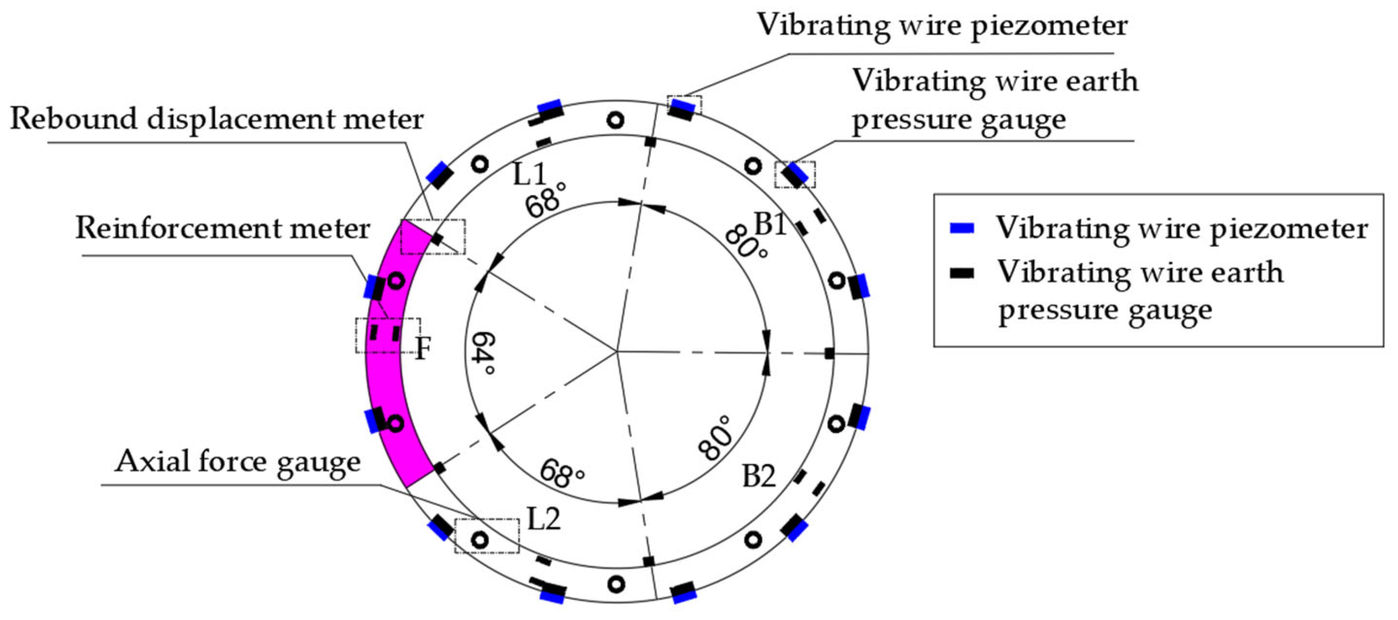
The project employs the shield tunneling method for construction. The inner diameter of the segment is 3000 mm, with a thickness of 250 mm and an outer diameter of 3500 mm. It employs staggered jointing. The ring wedge dimension for the connecting passage lining is 10.5 mm, with a ring width of 550 mm. The segments are prefabricated into five pieces (64° + 68° × 2 + 80° × 2), using concrete with a strength grade of C50. The cross-sectional diagram of the lining ring is shown in Figure 1. M24 bolts and curved bolts are used for connections between segments and between rings.
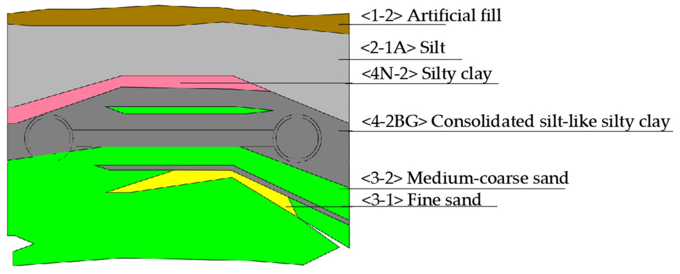
According to the geotechnical engineering exploration data, the overburden soil from top to bottom mainly consists of the following: artificial fill, silt, silt clay, consolidated silt-like silty clay, medium-coarse sand, and fine sand. The maximum water content of the water-rich sand layer is nearly 90%. For construction in the soft-soil bottom layer, the geological conditions are poor, surface settlement control is difficult, and the construction safety risk is high. The geological cross-section of the communication channel is shown in Figure 2.

2.2. Monitoring Plan

2.2.1. Monitoring Content

Based on similar engineering application experience and the principle of long-term reliability, the project utilized 12 vibrating wire earth pressure cells, model Gn-TY0106A, to measure earth pressure, 12 vibrating wire piezometers, model Gn-SY0206, to measure water pressure, 40 vibrating wire rebar stress meters, model HD-GJ1040, to measure steel stress, 20 axial force gauges, model YBY-M, to measure axial force, and 10 rebound displacement meters, model ATR-C, to measure the longitudinal joint opening amount.
Reasons for the 12-point layout of earth pressure and water pressure are as follows:
(1)
Symmetric coverage: The shield tunnel segments are axisymmetric structures, and theoretically, the load distribution is symmetrical. By arranging 12 measurement points at 30° intervals, the overall load pattern can be captured while also effectively identifying asymmetric conditions such as actual eccentric loading.
(2)
Key section control: The measurement points are laid out to cover mechanically sensitive areas such as the crown, haunch, and invert, ensuring effective monitoring of maximum internal forces and deformations.
(3)
Model robustness assurance: The data from 12 measurement points provide enough dimensionality to meet the basic requirements of regression analysis while avoiding the complexity issues caused by too many variables, ensuring the reliability of the results of the analysis.
The on-site monitoring measurement items and measurement tool parameters for the communication channel are shown in Table 1. The monitoring ring involves two monitoring sections at the front and rear, with the monitored segment ring marked as Ring M. The assembly point of the monitoring ring is set at the central position. All vibrating wire soil pressure gauges, vibrating wire sensor acquisition modules, and cables must incorporate waterproofing design to prevent leakage caused by sensor installation in the tunnel segments. Sensor protection is critical to survival rates; protection must be ensured throughout all stages of segment prefabrication. After installation, all sensors must remain within the geometric boundaries of the segment structure to prevent damage during shield machine assembly. Pre-embedded components and sensor installations should require on-site coordination with the manufacturer to ensure the integrity of the sensors in each installed segment. During construction, sensor positions may be adjusted based on specific segment reinforcement layouts, structural forms, and construction convenience. However, any changes to sensor quantities or technical parameters must be notified to and confirmed by the design unit. The cross-section of the cross-passage monitoring location is shown in Figure 3.
(1)
Earth pressure
Soil pressure refers to the effective stress exerted by the surrounding soil on the tunnel lining structure. A single row of vibrating wire earth pressure gauges, totaling 12 measuring points, was arranged on the Mth ring of the pipe ring, as shown in Figure 4 below. During the fabrication of the precast pipe sheets, a steel embedded box for the earth pressure gauge, measuring 240 mm × 140 mm × 32 mm, was pre-embedded. Installation precautions were as follows:
① To ensure the survival rate of the sensors, the earth pressure gauge and the wireless data gateway were installed after the pipe sheets were delivered to the site. The earth pressure gauge was connected to the pre-embedded cable via a conduit, ensuring waterproof sealing at the cable connection. During the fabrication of the precast pipe sheets, the lead-in cable was temporarily stored in the cable storage box and the embedded box. After installing the wireless data gateway and connecting the cable, the wireless data gateway was also placed inside the cable storage box.
② During the installation of the earth pressure gauge, we ensured that the outer surface of the earth pressure gauge was flush with the outer arc surface of the pipe sheet. The conduit was placed inside the embedded box. The interstitial space between the earth pressure gauge and conduit and the cable storage box was filled and compacted with rapid-hardening cement.
③ We inspected and tested the cables, cable concealing boxes, and sensors at time nodes, such as after segment prefabrication and sensor installation, to ensure the integrity and functionality of cables and sensors.
(2)
Water pressure
Water pressure refers to the hydrostatic pressure generated by groundwater acting on the outer surface of the pipe segment structure. A single row of vibrating wire piezometers was arranged on the Mth ring of precast pipe sheets, totaling 12 measurement points, as shown in Figure 5 below. During the fabrication of the precast pipe sheets, embedded boxes for the piezometers were pre-installed. These embedded boxes were made of steel and measured 250 mm × 60 mm × 32 mm. When installing the piezometers, it was essential to ensure that the permeable part of the piezometer was exposed. The remaining installation steps and precautions are highly consistent with the earth pressure measurement.
(3)
Axial force
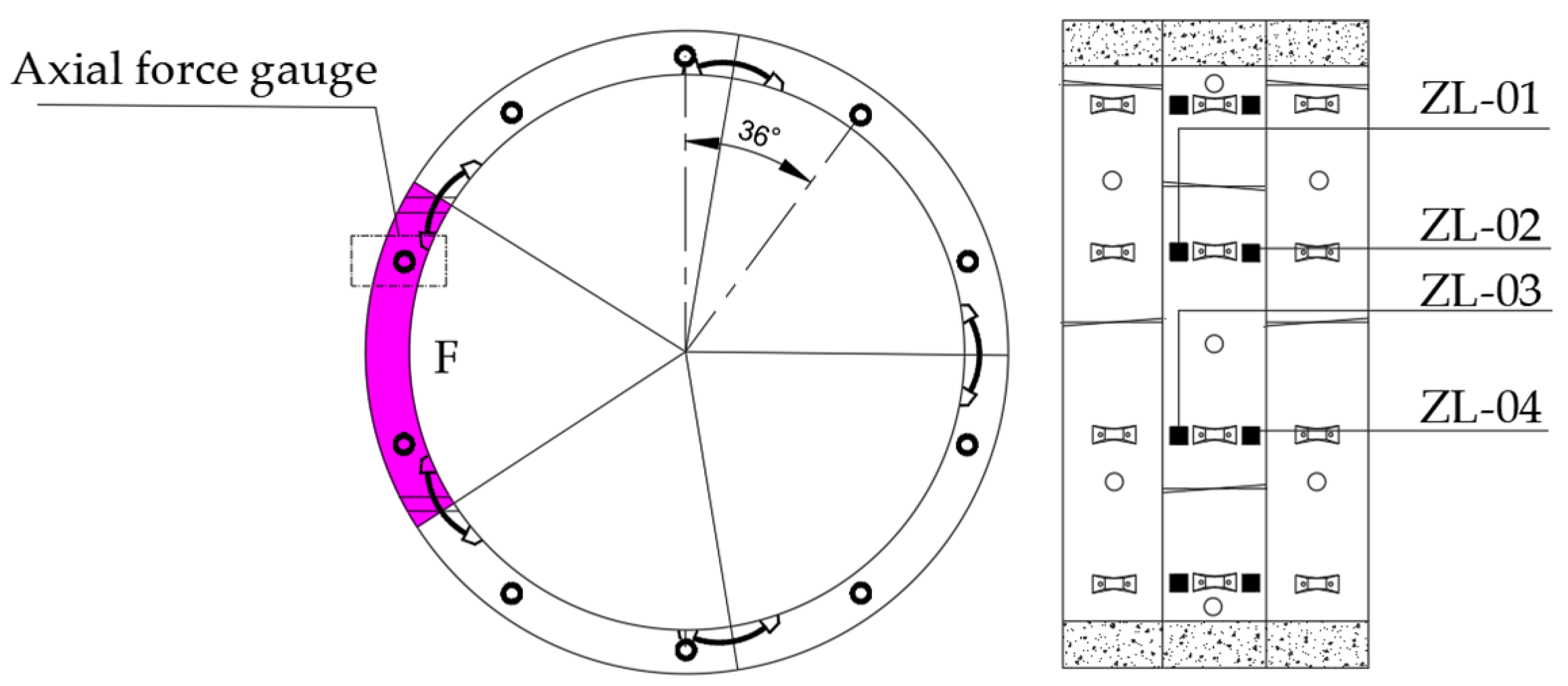
Segment axial force refers to the axial pressure acting on the centroid of the segment cross-section. It refers to the tension in the bolt, that is, the bolt clamping force. Axial force gauges are installed at longitudinal connecting bolts, with a spacing of 36° between each measurement point. The monitoring ring M-ring involves two monitoring sections (front and rear). Each monitoring section has 10 measurement points for monitoring the axial force of longitudinal bolts, as shown in Figure 6 below, requiring a total of 20 axial force gauges.
(4)
Reinforcement stress
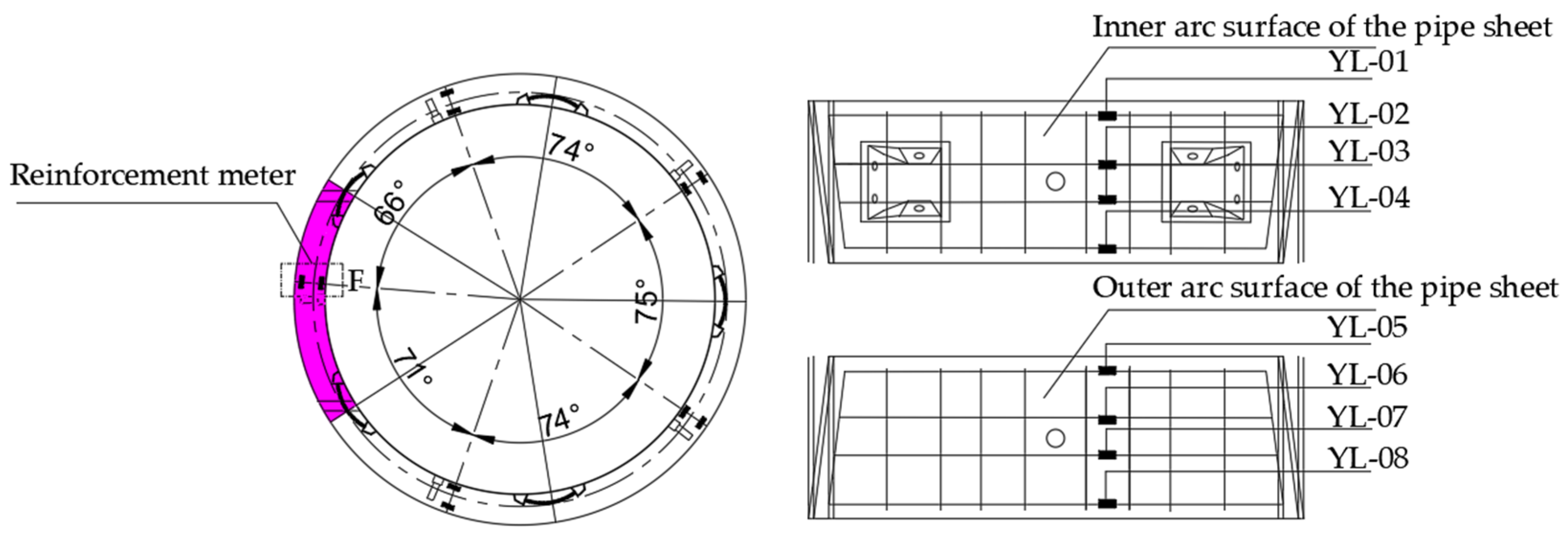
Reinforcement stress refers to the internal force borne per unit of cross-sectional area of the reinforcement embedded within reinforced concrete pipe segments under the action of external loads. The M-ring segment’s ring reinforcement bars are arranged on the inner and outer arc surface of the pipe sheet, with 5 measurement points on each side. Each point includes 4 reinforcement measurement sensors, totaling 40 measurement points, as shown in Figure 7 below. The installation precautions are as follows:
① When welding the reinforcement meter to the main reinforcement, cut the corresponding length at the installation position. Connect the reinforcement and the reinforcement meter’s matching rod with a coupler, and ensure the connection is fully welded around;
② During welding, take care not to damage or burn the cable. Pay special attention to avoid allowing the metal wire ends of the cable to contact the reinforcement mesh to be welded, as this may form a loop arc during welding and damage the reinforcement meter;
③ The assembly positioning points shown in the figure are for illustrative purposes only. The specific sensor positions on the segment should be determined on-site by the specialized unit according to construction conditions.
(5)
Longitudinal joint opening amount
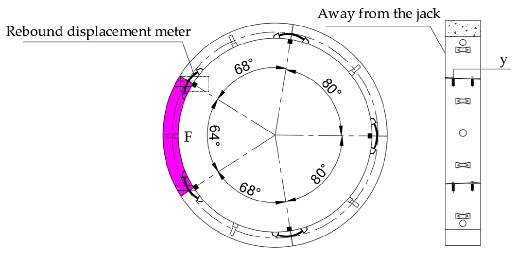
A total of five longitudinal joints within the segment ring of ring No.M are subject to surveillance, with two monitoring points per joint. Rebound displacement meters are installed on the inner arc surface of the pipe sheet. Each longitudinal joint has one monitoring point near the jack end and one away from the jack end. As shown in Figure 8 below, a total of 10 rebound displacement meters are required.
(6)
Sensor protection
Prior to reinforcing the cage binding, conduct visual inspections of cables, conduits, and junction boxes for integrity and functionality, and implement moisture protection measures. After concrete pouring, perform secondary inspections of cable joints and embedded components to ensure normal signal transmission. Upon arrival of precast segments at the site, conduct functional testing of each sensor individually and perform verification checks on installed sensors. Sensor status verification must be performed both before and after segment assembly. Protective signage must be installed during monitoring, and coordination with the construction team is required to jointly safeguard monitoring points.

2.2.2. Monitoring Results

In shield tunnel lining segments, the cap segment serves as the final closure component assembled. Its structural performance directly determines the overall mechanical behavior of the segment ring. Once the cap segment is installed, the segment ring transitions from an open state to a closed, pressure-bearing system. This enables effective transfer of circumferential loads and maintains stress equilibrium at the longitudinal joint; it has a decisive impact on the circumferential force system. As a critical load-bearing component in the monitored ring, the closure segment’s longitudinal joint opening behavior directly reflects the synergistic interaction mechanism between external loads and internal force systems. It is key to ensuring the continuity and integrity of this force flow path. This study focuses on the F cap block, a critical load-bearing component, and to prevent distortion from including too many collinear variables, it prioritizes selecting the directly corresponding monitoring points: two soil pressures, two water pressures, four axial forces, and eight rebar stress values as representative variables. For the ring segment F cap block of Ring 30, the daily average monitoring results for earth pressure, water pressure, and axial force are shown in Table 2. The reinforcement stress and longitudinal joint monitoring results are presented in Table 3.
Through the tabular data, we can observe that the reinforcement stress on the same level of the same segment exhibits a pattern wherein the inner side of the segment bears greater stress than the outer side. Bin Zhang [13] noted that at the crown line and tunnel bottom positions, the stress on the inner arc surface reinforcement exceeds that on the outer arc surface reinforcement, indicating that the inner arc surface reinforcement shoulders greater internal forces. This phenomenon also reveals the complexity of longitudinal and circumferential stresses within the segment ring. Potential reasons include the following: First, segments YL-01 and YL-05, positioned at the leading edge to bear the shield machine’s jack thrust, are directly situated at the starting point of the thrust transmission path, potentially exhibiting stress concentration (edge effect) [14,15]. Second, the stress mechanisms for inner and outer reinforcement differ fundamentally: the outer-arc reinforcement primarily bears compressive forces, while the inner-arc reinforcement (01) primarily bears tensile forces. Under the current loading conditions, compressive stress may significantly exceed tensile stress, resulting in higher readings for YL-05 compared to YL-01. Additionally, dynamic construction loads such as radial components from shield machine attitude adjustments, and grouting pressure, along with potential overall deformation of the segment ring (e.g., upward float), may exert more direct effects on the front-end section. This can cause redistribution of stresses during longitudinal transmission [16].

3. Multivariate Regression Analysis Based on SPSS

3.1. Normality Test

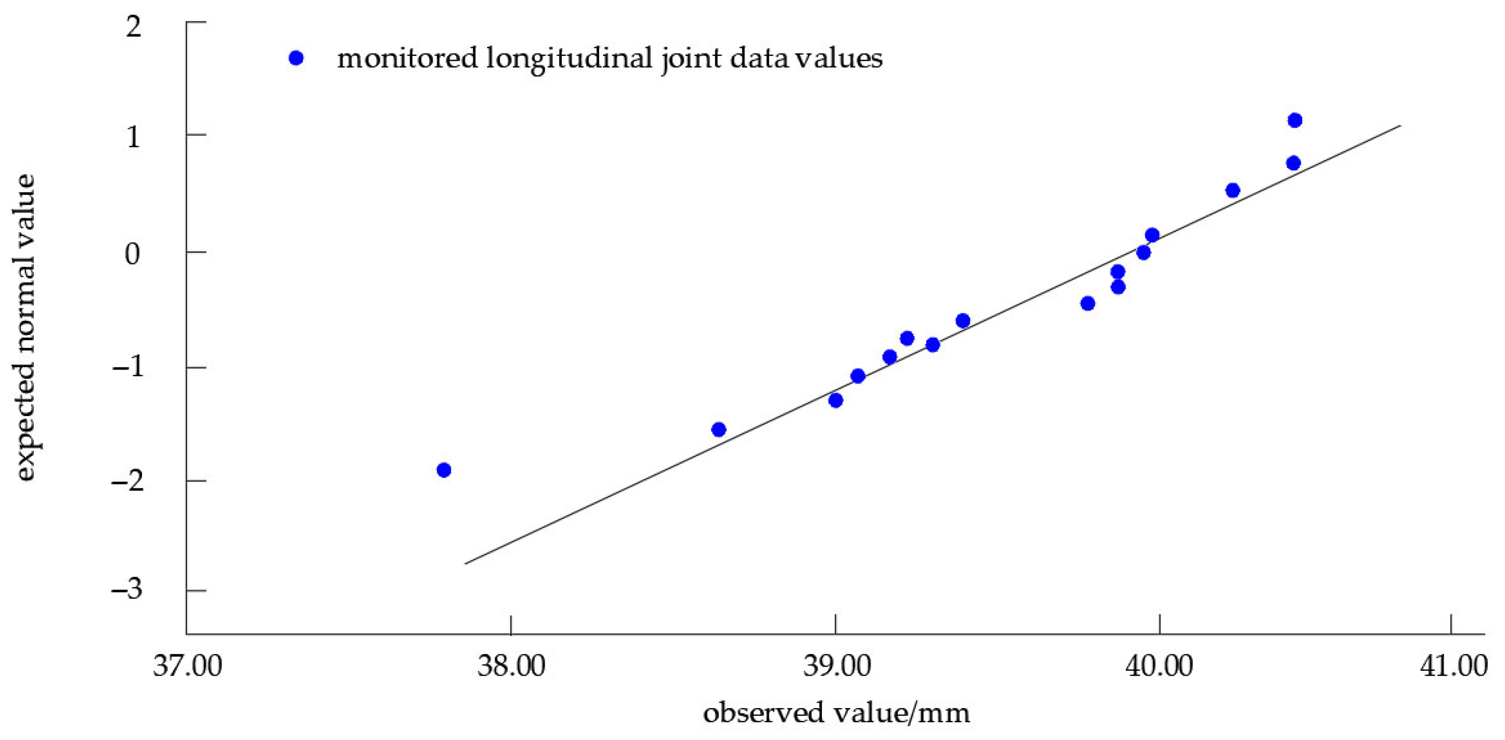
A normality test was conducted on the monitored longitudinal joint data values, and the results are shown in Table 4 below. Q-Q plots display the quantiles of sample data against the quantiles of a theoretical distribution in a scatter plot. If the sample data follows the theoretical distribution, these points should generally align along a straight line. Deviations from this line indicate that the sample data may not conform to the theoretical distribution. Since the data volume ≤ 50, the Shapiro–Wilk test results were used as the standard. The significance value was 0.18 > 0.05, and the normal distribution Q-Q graph of the longitudinal joint y opening amount is shown in Figure 9, indicating conformity to a normal distribution. Additionally, the monitoring data results are continuous numerical variables, so linear regression was selected for fitting.

3.2. Stepwise Linear Regression Analysis

3.2.1. Procedure of Stepwise Linear Regression Analysis

Regression analysis is used to study the interdependent relationships among multiple variables. Stepwise regression analysis is a method within multiple regression analysis, often employed to establish optimal or suitable regression models, thereby enabling a deeper exploration of the dependencies between variables. As a method for constructing optimal linear regression models, stepwise regression is straightforward and easy to implement. The resulting regression equation contains fewer variables while retaining the most significant and influential ones. In practice, this method has proven to be quite effective, offering high prediction accuracy. Furthermore, multiple variables often exhibit interrelationships, known as multicollinearity. Stepwise regression can, to a certain extent, correct for multicollinearity.
Stepwise linear regression is an automated process for selecting the optimal subset of predictor variables to construct a linear model. It progressively adds or removes variables through a series of steps based on specific statistical criteria. Its core process primarily involves three methods: forward selection, backward elimination, and bidirectional stepwise. The basic concept of the stepwise regression method is to automatically select the most important variables from a large number of available variables to establish a predictive or explanatory model for regression analysis. Its fundamental idea is to introduce independent variables one by one, with the condition that their partial regression sum of squares is significant after testing. Simultaneously, after each new variable is introduced, existing variables are tested one by one, and those with insignificant partial regression sum of squares are pruned. This process of introduction and elimination continues until no new variables can be introduced and no old variables need to be deleted. In essence, it aims to establish an “optimal” multiple linear regression (MLR) equation.
Stepwise regression in SPSS employs a bidirectional stepwise approach, combining forward selection and backward elimination. This is the most commonly used and automated method in practice. The Pearson Coefficient for data analysis is shown in Appendix A, and basic steps are as follows:
(1)
Data preparation. Import the data into SPSS, ensuring each variable is in a separate column and each observation is in a separate row. Confirm the measurement scale is correctly set in the Variable View: continuous for continuous variables, ordinal for ordinal, and nominal for categorical. The data in this paper are continuous variables, so select Scale.
(2)
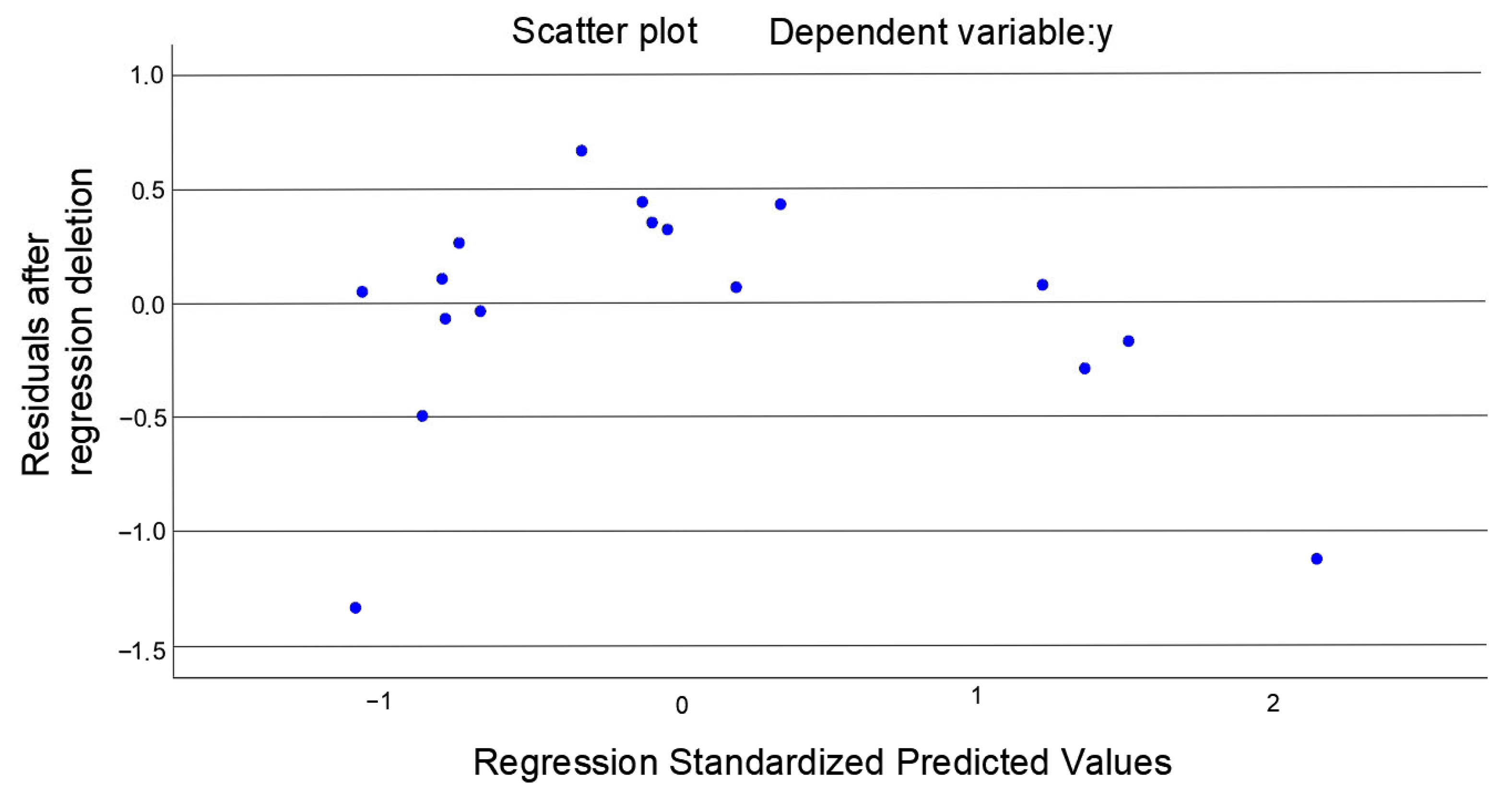
Preliminary analysis. Preliminary analysis of residual linearity, error independence, and homoscedasticity. The Durbin–Watson statistic is 2.2, indicating good independence of residuals. The scatter plot of standardized residuals is uniformly distributed around the origin, confirming good homoscedasticity. Run descriptive statistics by selecting Analyze, Descriptive Statistics, and Frequency. Review the mean and standard deviation, and check for outliers. Run correlation analysis by selecting Analyze, Correlation, and Bivariate. Initially examine the correlations between the independent variables and the dependent variable, as well as among the independent variables themselves. Be alert to highly correlated independent variables, which indicate potential multicollinearity.
(3)
Variable and method selection. Select Analyze, Regression, and Linear. Place the vertical joint opening into the Dependent Variable box and select earth pressure, water pressure, axial force, and reinforcement stress in the Independent Variable box. Allow SPSS to automatically screen variables based on the statistical significance of the F-value.
(4)
Select required statistics. Choose to output regression coefficients B, standard errors, significance levels, R, R2, variance inflation factors, and other relevant statistics.
(5)
Run the multiple regression analysis.
Using multiple linear regression (MLR) analysis, we directly set the raw voltage signal from the rebound displacement meter as the dependent variable y, while earth pressure, water pressure, axial force, and steel stress were set as independent variables, TY, SY, ZL, and YL, respectively. This approach aims to maximally preserve the original statistical characteristics of the measurement data and to avoid potential nonlinear distortions or changes in variance structure that could be introduced by converting to physical units through calibration, thereby ensuring the unbiasedness and effectiveness of subsequent regression analysis results. The rebound-type displacement meter used in this study operates on the principle of detecting external loads through deformation of its internal spring. Its raw readings have a direct, one-to-one mapping relationship with the mechanical state applied to the segment joints (such as reduced clamping force or increased opening force). Therefore, using the raw readings to build statistical models with factors such as grouting pressure and jack thrust essentially establishes the relationship between the ‘joint stress state’ and these external factors, which holds more direct physical significance than using the converted absolute displacement values. Our target prediction is the longitudinal joint trend.
SPSS Statistics 27 software was employed to analyze the functional relationships between the independent variables and multiple dependent variables. During the analysis process, axial force and steel stress were automatically excluded. The stepwise linear regression analysis Table 5, regression coefficient Table 6, and regression variance Table 7 are shown as follows.

3.2.2. Results and Analysis of Stepwise Linear Regression

After automatic model identification, two variables, SY-01 and TY-02, remained in the model. R2 indicates the percentage of variation in the dependent variable Y that the model can account for. The value of R2; ranges from 0 to 1. R2 = 0 means that the model cannot explain any variation in the dependent variable and is ineffective; R2 = 1 means that the model perfectly explains all variation in the dependent variable, with all data points lying exactly on the regression line. R2 = 0.5 indicates that the model explains approximately 50% of the variation in the dependent variable, with the remaining variation unexplained by the model and attributed to other, unknown factors or random error. F is used to compare the ratio of two variances, thereby determining whether there are significant differences in the mean or explanatory power between different groups or among multiple predictor variables. A larger F-value indicates a greater likelihood that observed differences are genuinely present; a smaller F-value, closer to 1, suggests no significant differences exist between the selected data groups. VIF is a measure of the severity of multicollinearity among independent variables in a linear regression model. It quantifies how much the variance of the regression coefficient estimate for one independent variable increases due to the correlation between other independent variables. VIF = 1 indicates that the independent variable is completely uncorrelated with the others. Alternatively, 1 < VIF < 5 indicates mild multicollinearity, generally considered acceptable; 5 ≤ VIF < 10 indicates moderate multicollinearity, which may warrant attention; and VIF ≥ 10 indicates severe multicollinearity. The regression coefficient estimate for this independent variable is unreliable, statistical power is reduced, and intervention is required. The p-value represents the probability of observing the current sample data or more extreme data under the null hypothesis. p ≤ 0.01 indicates extreme significance, providing very strong evidence supporting the alternative hypothesis. A value of 0.01 < p ≤ 0.05 signifies significance, indicating strong evidence supporting the alternative hypothesis. A value of 0.05 < p ≤ 0.10 denotes marginal significance, suggesting weaker evidence but warranting attention, potentially requiring additional data. Finally, p > 0.10 indicates non-significance, meaning that insufficient evidence supports the alternative hypothesis. The t-value is a statistic measuring the magnitude of the difference between an estimated value and its hypothesized value relative to the sampling error of that estimate. It must be interpreted in conjunction with the p-value.
Further detailed analysis showed that the regression coefficient of x 21 was 0.032 (t = 5.287, p < 0.001), indicating a significant positive influence on the longitudinal joint y. The regression coefficient of TY-02 was −0.024 (t = −2.682, p = 0.018), indicating a significant negative influence on the longitudinal joint y. The regression equation is as follows: Y = 40.348 + 0.032 ( S Y 01 ) 0.024 ( T Y 02 ) .
Based on the multiple linear regression model, the monitoring results of the longitudinal joint y between segments B2 and B1 in the 30th ring of the liaison tunnel were tested. The corresponding water pressure and earth pressure values at the positions of segments B2 and B1 were substituted into the model and compared with the actual data. The fitting results are shown in Figure 10, where the measured values generally align with the predicted values.

4. Conclusions

(1)
The influence of internal forces within the segment on longitudinal joint opening is relatively minor. Within the context of the regression model developed for this specific dataset, external pressure variables were found to be statistically more significant predictors of longitudinal joint opening than measured internal force variables. Specifically, longitudinal joint opening increases with rising water pressure and decreases with increasing earth pressure. Although the statistical method excluded the significance of axial force, this contradicts engineering intuition. Analysis suggests that the result is more likely due to data characteristics or modeling limitations: during construction, axial force is affected by transient factors, resulting in noisy data and high correlation with external loads, which leads the model to prioritize more stable proxy variables. This finding indicates that the mechanical importance of axial force is not negated, but caution is required when interpreting data-driven models due to construction disturbances.
(2)
A stepwise linear regression analysis method was adopted, resulting in a linear regression equation for water pressure and earth pressure as Y = 40.348 + 0.032 ( S Y 01 ) 0.024 ( T Y 02 ) , with a coefficient of determination R2; of 0.697. The error is 30.3%.
(3)
By fitting the monitoring data and predicted data for the 30th ring segment, the model demonstrated excellent agreement with the monitoring data. This research outcome provides a case-specific reference for structural safety control in analogous geological and construction conditions, though its generalizability requires further validation with long-term multi-ring data.
(4)
This study has certain limitations. The analysis primarily relies on data from a single monitoring ring during a specific construction phase, potentially failing to fully capture the complex nonlinear relationships and multi-factor interactions between water and soil pressures and structural responses in shield tunnels. These factors may affect the model’s universality and predictive accuracy under broader geological conditions or different construction scenarios. Future research should focus on establishing a large-scale, standardized database covering diverse geological conditions and the entire construction cycle. Building upon this foundation, actively incorporating nonlinear models or machine learning algorithms could enable more precise characterization of the complex mechanisms governing longitudinal joint opening.
(5)
It must be acknowledged that two-dimensional regression models based on single-ring data have inherent limitations in capturing the complex three-dimensional mechanical behavior of intersecting channels (such as longitudinal bending and inter-ring load transfer). Subsequent work will introduce three-dimensional numerical analysis and multi-ring synchronous monitoring to reveal its spatial mechanical mechanisms.

Author Contributions

S.L.: Determined the current research status on the opening width of longitudinal seams, and clarified the research gaps in earth pressure and water pressure. Described engineering parameters and assisted in extracting key conclusions. Checked the consistency of monitoring data tables, standardized statistical terms, and adjusted the manuscript’s logic. J.H.: Provided detailed descriptions of sensor models, layout, and installation in the monitoring plan; interpreted the normality test; and explained the steps of regression analysis. Verified the calculations of the regression equation, reviewed sensor protection measures, and standardized the format of references. Y.G.: Determined the bidirectional stepwise multiple linear regression method, designed a multi-parameter monitoring system, and used the Shapiro–Wilk test to check the normality of the longitudinal seam data. L.Z.: Organized the monitoring data into a dataset, calculated normality and key regression metrics, and drew a longitudinal seam fitting chart to validate the regression equation. W.Z.: Interpreted the regression results, explained the function of the capping block, and assisted in elaborating on the engineering value. Reviewed and revised, checked the correspondence between measurement point diagrams and text, verified the longitudinal seam fitting diagram, and standardized data units. All authors have read and agreed to the published version of the manuscript.

Funding

This research received no external funding.

Data Availability Statement

Due to the high cost of obtaining the data, these data are not publicly available. The data presented in this study can be obtained from the corresponding author upon request.

Conflicts of Interest

Authors Shuqiang Li, Jianzhong Hao, Yunchang Gao and Lei Zhang authors are employed by the Qingdao Metro Line 8 Co., Ltd. The remaining author declares that the research was conducted in the absence of any commercial or financial relationships that could be construed as a potential conflict of interest.

Appendix A

Pearson Coefficient
TY-01TY-02SY-01SY-02ZL-01ZL-02ZL-03ZL-04YL-01YL-02YL-03YL-04YL-05YL-06YL-07YL-08y
TY-0110.683 **0.4190.526 *−0.1850.1070.384−0.0520.4010.370.2540.030.0660.487 *0.640 **0.316−0.038
TY-020.683 **10.1190.199−0.585 *0.2030.2940.1230.619 **0.730 **0.694 **0.099−0.0140.834 **0.791 **0.621 **−0.725
SY-010.4190.11910.982 **0.609 **0.0470.015−0.101−0.293−0.547 *−0.607 **−0.0560.549 *−0.3130.044−0.3870.736 **
SY-020.526 *0.1990.982 **10.512 *0.0520.007−0.041−0.224−0.458−0.530 *−0.0940.504 *−0.20.146−0.30.696 **
ZL-01−0.185−0.585 *0.609 **0.512 *10.14−0.176−0.079−0.469−0.860 **−0.888 **−0.2350.261−0.764 **−0.512 *−0.569 *0.598 *
ZL-020.1070.2030.0470.0520.141−0.0540.4050.4770.10.104−0.581 *−0.542 *0.2760.3260.482−0.202
ZL-030.3840.2940.0150.007−0.176−0.0541−0.799 **0.1290.2840.2850.535 *0.1030.2060.052−0.024−0.097
ZL-04−0.0520.123−0.101−0.041−0.0790.405−0.799 **10.4310.1320.118−0.794 **−0.513 *0.2920.4230.557 *−0.235
YL-010.4010.619 **−0.293−0.224−0.4690.4770.1290.43110.773 **0.749 **−0.383−0.705 **0.835 **0.815 **0.948 **−0.541 *
YL-020.370.730 **−0.547 *−0.458−0.860 **0.10.2840.1320.773 **10.987 **0.109−0.4010.928 **0.684 **0.812 **−0.707 **
YL-030.2540.694 **−0.607 **−0.530 *−0.888 **0.1040.2850.1180.749 **0.987 **10.125−0.4250.907 **0.632 **0.796 **−0.710 **
YL-040.030.099−0.056−0.094−0.235−0.581 *0.535 *−0.794 **−0.3830.1090.12510.662 **−0.094−0.282−0.4540.053
YL-050.066−0.0140.549 *0.504 *0.261−0.542 *0.103−0.513 *−0.705 **−0.401−0.4250.662 **1−0.424−0.38−0.719 **0.532 *
YL-060.487 *0.834 **−0.313−0.2−0.764 **0.2760.2060.2920.835 **0.928 **0.907 **−0.094−0.42410.845 **0.890 **−0.557 *
YL-070.640 **0.791 **0.0440.146−0.512 *0.3260.0520.4230.815 **0.684 **0.632 **−0.282−0.380.845 **10.814 **−0.251
YL-080.3160.621 **−0.387−0.3−0.569 *0.482−0.0240.557 *0.948 **0.812 **0.796 **−0.454−0.719 **0.890 **0.814 **1−0.599 *
y−0.038−0.72 **0.736 **0.696 **0.598 *−0.202−0.097−0.235−0.541 *−0.707 **−0.710 **0.0530.532 *−0.557 *−0.251−0.599 *1
* denotes p < 0.05, and ** indicates p < 0.01.
Figure A1. Residuals vs. predicted values. The correlation analysis results between variables indicates that the longitudinal joint opening y exhibits a highly positive correlation with water pressure SY-01 (correlation coefficient 0.736, p < 0.01) and a significant negative correlation with earth pressure TY-02 (−0.72, p < 0.05). Furthermore, some independent variables exhibit high correlation; for instance, the correlation coefficient between SY-01 and SY-02 reaches 0.982, indicating they provide nearly redundant information. This strong correlation among independent variables (i.e., multicollinearity) is a critical consideration when performing stepwise regression analysis.
Buildings 15 04175 g0a1

References

  1. Yang, J.; Chen, W.-Z.; Li, M.; Tan, X.-J.; Yu, J.-X. Structural Health Monitoring and Response Pattern Analysis of Underwater Shield Tunnels During Operation. J. Rock Mech. Eng. 2021, 40, 902–915. [Google Scholar]
  2. Wang, R. Analysis of Deformation Factors and Characteristics in Shanghai’s Soft Soil Subway Tunnels. Undergr. Eng. Tunneling 2009, 7, 1–6+52. [Google Scholar]
  3. Han, S. Analysis of Causes and Countermeasures for Cracking in Shield Tunnel Segments. West. Explor. Eng. 2010, 22, 151–153. [Google Scholar]
  4. Hong, W.; Wang, F. Unified Phase-Field Simulation and Toughness Evaluation of Crack Damage Evolution in Shield Tunnels Through Saturated Soft Soil. J. Geotech. Eng. 2025, 40, 1–10. [Google Scholar]
  5. Zhang, W.; Yang, Q.; Li, Y.; Dong, Z.; Wang, X. Design and mechanical properties of special segment structure in mechanical connecting aisle. Structures 2024, 64, 106589. [Google Scholar] [CrossRef]
  6. Wang, Z.; Zhao, Y.; Zhang, S.; Gao, Y. Risk analysis of mechanical cross-passage construction using work breakdown and fault tree. Proc. Inst. Civ. Eng. Forensic Eng. 2025, 178, 8–17. [Google Scholar] [CrossRef]
  7. Wang, X.; Chen, C. Vibration Table Test of Prefabricated L-Shaped Column Concrete Structure. Buildings 2025, 15, 2329. [Google Scholar] [CrossRef]
  8. Chen, P.; Geng, P.; Chen, C. A Study on the Mechanical Model of Shield Tunnel Segment Joints Considering Joint Positive Contact Nonlinearity. Acta Civilia Ingeniae Sin. 2021, 54, 87–97. [Google Scholar]
  9. Sun, F.; Li, W.; Li, C. Relationship between Longitudinal joint Opening and Convergence Deformation in Cross-River Shield Tunnels. J. Undergr. Space Eng. 2023, 19, 309–318. [Google Scholar]
  10. Xu, C.; Wang, S.; Xia, C.; Liu, L.; Ma, Z.; Yang, J. Viscoelastic plastic interaction of tunnel support and strain-softening rock mass considering longitudinal effect. Rock Mech. Bull. 2024, 3, 100152. [Google Scholar] [CrossRef]
  11. Xu, C.; Wang, S.; Xia, C. Analytical prediction for time-dependent interaction of a circular tunnel excavated in strain-softening rock mass. Rock Mech. Bull. 2024, 3, 100127. [Google Scholar] [CrossRef]
  12. Xu, C.; Xia, C. A new large strain approach for predicting tunnel deformation in strain-softening rock mass based on the generalized Zhang-Zhu strength criterion. Int. J. Rock Mech. Min. Sci. 2021, 143, 104786. [Google Scholar] [CrossRef]
  13. Zhang, B. Monitoring and Analysis of Stress Characteristics in Large-Diameter Shield Tunnel Segments Crossing Rivers. Railw. Constr. Technol. 2022, 184–188. [Google Scholar]
  14. Mu, H.; Kun, F.; Guo, W. Study on Structural Mechanical Behavior and Failure Characteristics of Segments in Ultra-Large-Diameter Shield Tunnels. Mod. Tunn. Technol. 2025, 62, 125–134. [Google Scholar]
  15. Sun, F. Analysis of Causes and Prevention Measures for Segment Misalignment in Shield Construction. Sichuan Cem. 2018, 294. [Google Scholar]
  16. Ni, Z.; Wang, S.; Hang, S. Influence of Upper Shield Tunneling in Water-Rich Gravel Formations on the Mechanical State of Lower Segments in Diagonally Parallel Tunnels. J. Cent. South Univ. (Nat. Sci. Ed.) 2022, 53, 2996–3007. [Google Scholar]
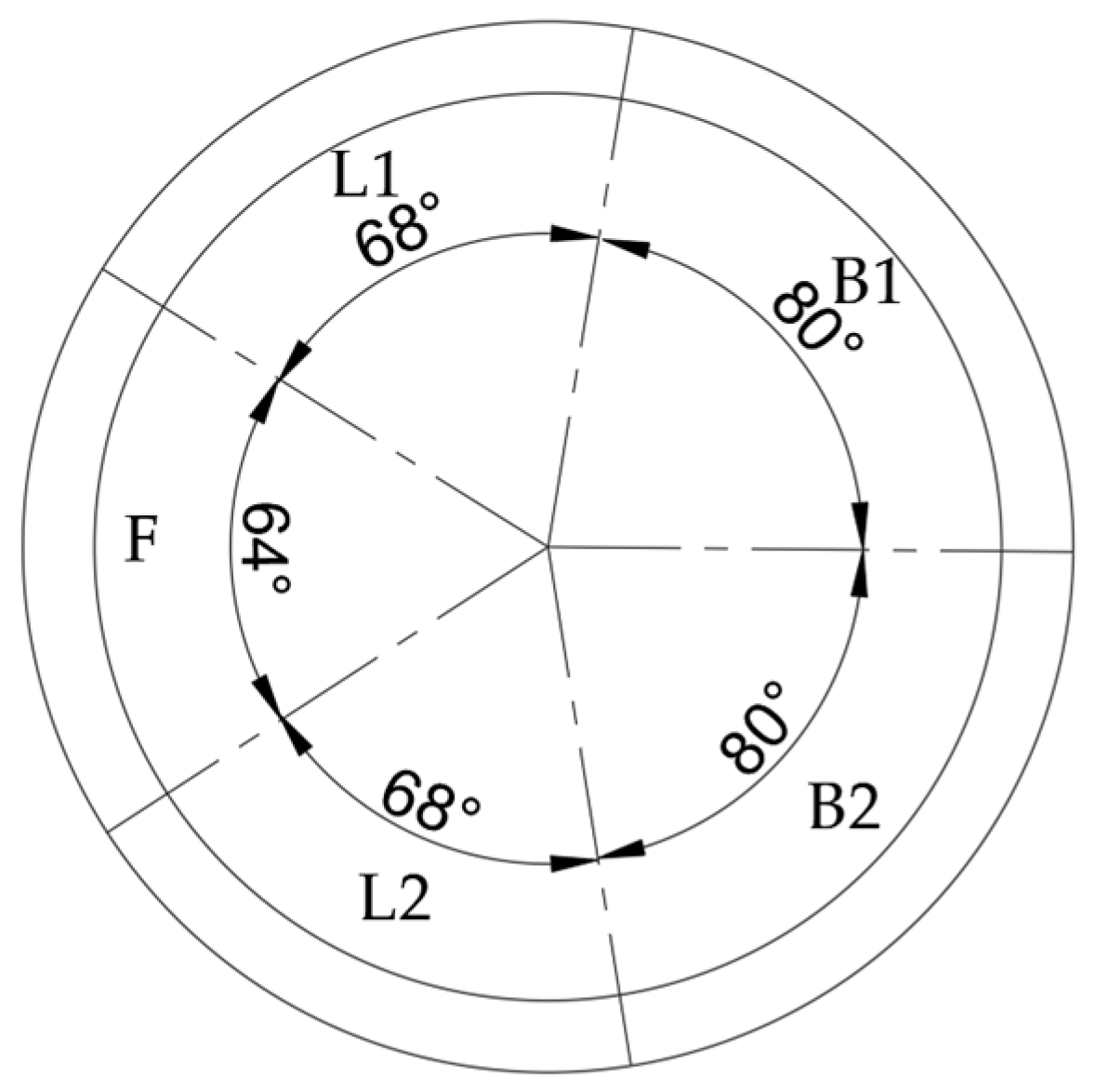
Figure 1. Cross-section of the lining ring. F denotes the cap block, L1 and L2 denote adjacent blocks, and B1 and B2 denote standard blocks.
Buildings 15 04175 g001
Figure 2. Geological profile of the communication channel.
Buildings 15 04175 g002
Figure 3. The cross-section of the cross-passage monitoring location.
Buildings 15 04175 g003
Figure 4. Layout diagram of measuring points for the 30th ring’s earth pressure. Note: The highlighted section indicates the F capping block. TY-01 and TY-02 represent the soil pressure monitoring points for the F capping block. The angle formed between two adjacent vibrating wire soil pressure gauges was 30°, with the sensors positioned at the center of the segment width and the precast box installed between the two sensors.
Buildings 15 04175 g004
Figure 5. Layout diagram of piezometric measurement points for Ring 30. The highlighted section indicates the F capping block. SY-01 and SY-02 are the water pressure monitoring points for the F capping block. The angle formed between two adjacent vibrating wire piezometers is 30°, with the sensors oriented toward the tunnel lining. The pre-embedded box is positioned between the two sensors.
Buildings 15 04175 g005
Figure 6. Layout of longitudinal Bolt Measuring Points between Ring M-1 and Ring M, and between Ring 30 and Ring 30+1. The angle formed between two adjacent axle load sensors is 36°.The highlighted sections represent F cap blocks. ZL-01, ZL-02, ZL-03, and ZL-04 are axial force monitoring points for the F cap blocks.
Buildings 15 04175 g006
Figure 7. Layout diagram of stress measuring points for reinforcement in ring 30. The highlighted section represents the F-type cap block. YL-01, YL-02, YL-03, and YL-04 denote the inner reinforcement stress gauges within the F-type cap block, while YL-05, YL-06, YL-07, and YL-08 denote the outer reinforcement stress gauges. The dotted box indicates a vibrating wire type reinforcement gauge.
Buildings 15 04175 g007
Figure 8. Layout of measuring points for longitudinal joint opening at Ring 30. The highlighted section represents the F capping block, and y denotes the vertical joint opening monitoring point for the F capping block and the adjacent L1 block.
Buildings 15 04175 g008
Figure 9. Normal Q-Q Plot of Longitudinal Seam y.
Buildings 15 04175 g009
Figure 10. Fitting effect diagram of longitudinal seam y.
Buildings 15 04175 g010
Table 1. Tunnel site monitoring measurement items and measurement tool parameters.
Serial NumberMonitoring ParametersSensor NameModelRangeResolution
1Earth pressureVibrating wire soil pressure gaugeGn-TY0106A0~1.6 (MPa)<0.05 F.S.
2Water pressureVibrating wire piezometerGn-SY02060~1.0 (MPa)<0.05 F·S
3Axial forceAxial force gaugeYBY-M0~500 (kN)
4Reinforcement stressVibrating wire rebar gaugeHD-GJ1040<800 (MPa)<0.05 F·S
5Longitudinal joint opening amountRebound displacement gaugeATR-C±50 mm±0.1 mm
Table 2. Earth pressure, water pressure, and axial force surveillance results.
Date (yyyy-mm-dd)Earth Pressure (MPa)Water Pressure (MPa)Axial Force Monitoring Results (KN)
TY-01TY-02SY-01SY-02ZL-01ZL-02ZL-03ZL-04
2024-10-02265.74269.69203.85203.2090.2116.232.3247.70
2024-10-03271.89268.46205.67203.2889.7815.897.8234.90
2024-10-04269.53270.36201.56197.0489.6116.067.4834.11
2024-10-06289.88302.21242.94236.9686.4014.187.6534.29
2024-10-07258.26267.30179.29174.8188.3513.676.5334.11
2024-10-08265.92276.02180.39183.4338.8913.496.5333.76
2024-10-09270.88275.54181.02184.5038.893.506.7034.11
2024-10-10269.73302.05208.05203.6638.8914.436.6237.97
2024-10-11279.23288.65189.13192.7938.8914.696.3637.71
2024-10-12276.36300.80194.23195.6038.8915.127.0538.32
2024-10-14271.79296.98183.40186.7338.8915.376.7038.41
2024-10-15272.57288.09178.21185.6738.8915.806.7938.76
2024-10-16273.82290.78177.71184.2338.8915.896.8738.67
2024-10-17275.48289.72177.15183.4938.8915.896.8738.50
2024-10-18277.03294.41175.18178.6938.8915.976.8738.58
2024-10-19273.53289.30175.24177.7938.8915.976.8738.76
2024-10-20274.66293.25173.84177.1738.8916.066.9638.76
Table 3. Reinforcement stress and longitudinal joint surveillance results.
Date (yyyy-mm-dd)Reinforcement Stress (MPa)Longitudinal Joint (mm)
YL-01YL-02YL-03YL-04YL-05YL-06YL-07YL-08y
2024-10-0211.4613.7911.7814.468.932.813.522.6940.23
2024-10-0311.5013.9812.3015.188.862.733.312.3440.41
2024-10-0411.4414.0912.6416.238.962.733.312.0740.42
2024-10-0611.4014.8913.1316.599.853.353.732.2240.54
2024-10-0711.3314.8313.9716.629.332.742.982.2539.78
2024-10-0810.5914.7614.0816.989.512.873.031.7139.87
2024-10-0911.1315.4014.7616.999.463.043.302.0139.87
2024-10-1011.8615.7815.8616.239.353.773.992.8940.16
2024-10-1112.1216.3416.0915.908.873.784.103.2539.95
2024-10-1212.3116.2716.7816.068.924.034.113.4139.98
2024-10-1412.0216.3916.8515.708.883.893.553.2539.39
2024-10-1512.0316.3816.5715.618.834.183.923.4439.17
2024-10-1612.1416.4716.7215.988.834.033.773.3839.22
2024-10-1712.4316.5316.8016.108.853.903.813.2439.07
2024-10-1812.1816.5916.7615.868.843.853.923.3239.00
2024-10-1912.2016.4116.7715.878.843.753.753.3738.64
2024-10-2012.1216.4116.6115.938.743.753.723.2137.79
Table 4. Normality test of longitudinal joint y.
Kolmogorov–SmirnovaShapiro–Wilk
StatisticdfSignificanceStatisticdfSignificance
y0.176170.1670.925170.180
Table 5. Stepwise linear regression analysis table.
Regression ModelModel
Variables
Determination
Coefficient/R2
Standard
Error of
Estimate
Significance Change
1SY-010.5420.512<0.001
2SY-01
TY-02
0.6970.4310.018
Table 6. Regression coefficients table.
ModelUnstandardized CoefficientsStandardized CoefficientstSignificanceCollinearity Statistics
BStd. ErrorBetaToleranceVIF
1(Constant)33.9461.353-25.090<0.001--
SY-010.0300.0070.7364.209<0.0011.0001.000
2(Constant)40.3482.645-15.256<0.001--
SY-010.0320.0060.7835.287<0.0010.9861.014
TY-02−0.0240.009−0.397−2.6820.0180.9861.014
Table 7. Regression variance table.
ModelSum of SquaresdfMean SquareFSignificance
1Regression 4.64314.64317.716<0.001
Residual3.931150.262
Total8.57516-
2Regression 5.97722.98916.110<0.001
Residual2.597140.186
Total8.57516-
Disclaimer/Publisher’s Note: The statements, opinions and data contained in all publications are solely those of the individual author(s) and contributor(s) and not of MDPI and/or the editor(s). MDPI and/or the editor(s) disclaim responsibility for any injury to people or property resulting from any ideas, methods, instructions or products referred to in the content.