Machine Learning Prediction on Progressive Collapse Resistance of Purely Welded Steel Frames Considering Weld Defects

Abstract

This study proposes a machine learning (ML) framework to predict the progressive collapse resistance of purely welded steel frames considering weld defects. A finite element model (FEM) incorporating weld weakening degree at joints was developed and validated against push-down tests. A parametric modelling program, combined with Latin Hypercube Sampling (LHS), was used to generate 700 samples from 27 design features across 8 categories, establishing a progressive collapse database containing full-process resistance curves. Five ML algorithms—DNN, SVR, RF, XGBoost, and LightGBM—were trained and evaluated. SVR was identified as the optimal model through Bayesian hyperparameter optimization and K-fold cross-validation, achieving an R² = 0.988 and sMAPE = 5.096% in predicting the full-process resistance response. SHAP analysis was employed to examine feature interpretations both locally and globally, revealing that the failure scenario, beam span-to-height ratio, and weld quality are the three most significant factors affecting structural resistance, accounting for 22.6%, 22.5%, and 16% of the overall influence, respectively. For practical design, a steel frame with a beam span-to-height ratio of approximately 15, a weld joint relative position ratio between 0.15 and 0.18, a circular stub diameter-to-beam width ratio around 1.8, and a stub diameter-to-thickness ratio near 13 can achieve superior progressive collapse robustness, provided that weld quality is ensured.

1. Introduction

Progressive collapse of structures represents one of the most catastrophic events in civil engineering. The September 11 attacks in the United States, for instance, caused massive casualties and economic losses, exposing the vulnerability of modern structures to multiple extreme hazards and revealing the limitations of conventional design guidelines in addressing unexpected accidental loads. The triggers of progressive collapse are diverse. When a structure is subjected to extreme loads such as explosions or vehicle impacts, the directly affected components sustain initial damage, which may then propagate to adjacent areas. As structural redundancy becomes insufficient, internal forces are redistributed through alternative load paths, ultimately leading to extensive failure or total collapse under applied loads [1]. The root causes often lie in insufficient structural robustness and ductility, coupled with a lack of effective alternate load paths (ALP) [2,3], which collectively fail to contain localized damage propagation. Therefore, developing efficient evaluation methods to enhance structural resistance to progressive collapse under accidental events remains an important research objective.

Steel frames are widely used in modern structures due to their superior strength, ductility, and construction efficiency. According to the ALP design philosophy [4], the load-carrying capacity and ductility of a representative substructure—extracted between bending inflection points of the remaining frame under the combined action of column-top loading and uniformly distributed beam loads—can be taken as indicative of the overall structural resistance to progressive collapse following the sudden removal of a critical column [5,6]. Based on this concept, many researchers have conducted quasi-static push-down tests on single-bay planar substructures to investigate resistance mechanisms and load transfer under the column removal scenario.

Research shows that beam-column joint configuration significantly influences substructural resistance and ductility, particularly in determining whether effective catenary action (CA) can develop. Yang et al. [7] and Oosterhof et al. [8] performed push-down tests and demonstrated that bolted web angle connections can effectively mobilize both flexural action (FA) and catenary action (CA). Weigand et al. [9] observed that although such connections reduce the initial load-carrying capacity compared to welded-bolted connections, they exhibit superior ductility, albeit with a need for enhanced shear resistance. Dinu et al. [10] reported that welded cover plate flange connections (CWP), haunched end-plate bolted connections (EPH), and reduced beam section (RBS) welded connections all achieve excellent ductility and capacity through CA. Zhong et al. [11,12] further indicated that the resistance of rigid joints (e.g., welded flange–bolted web connections) is dominated by FA, whereas that of semi-rigid joints (e.g., bolted web angle connections) is primarily provided by CA. Zhang et al. [13] and Qian et al. [14,15] also emphasized the crucial influence of semi-rigid connection details on load capacity and ductility. Additionally, all-welded beam-column joints represent another common configuration. Yu and Huang et al. [16,17] highlighted that weld quality significantly affects resistance development. Poor welding can trigger sudden fracture of the flange or web under small deformations, resulting in abrupt loss of load capacity, which critically governs substructural ductility and overall robustness.

Beyond joint behavior, structural design parameters—such as beam and column cross-sectional dimensions, span-to-height (STH) ratio, height-to-width (HTW) ratio, and boundary conditions—also considerably influence substructural performance across different resistance stages. Yang et al. [18,19] indicated that increasing the beam cross-section or reducing the STH ratio enhances FA but impairs CA development. A higher HTW ratio makes the web and flange more prone to local buckling, weakening FA and hindering CA [20]. Huang et al. [21] suggested that under push-down loading, substructures with higher boundary stiffness exhibit greater load capacity but reduced ductility. Inadequate horizontal restraint can induce significant lateral displacement in corner columns, which is detrimental to progressive collapse resistance.

The studies referenced above rely primarily on experimental and numerical approaches. Experimentally validated numerical models allow for efficient parametric studies, an approach also widely applied in steel–concrete composite structure analysis [22,23,24,25]. However, when analyzing the progressive collapse resistance of steel frames while simultaneously accounting for multiple design parameters—especially weld uncertainty at joint locations—traditional parametric methods fall short in enabling rapid performance prediction and design feedback.

The rapid development of artificial intelligence, particularly machine learning (ML), has demonstrated strong performance in materials design [26,27,28] and offers a promising alternative for structural performance prediction. In the context of progressive collapse, Zhu et al. [29] developed an efficient machine learning algorithm to assess the effects of damping ratio, column removal time, and structural period on the dynamic amplification factor (DAF), providing an innovative instrument for quantifying dynamic effects in nonlinear static analysis. Guo [30] employed multiple ML models to predict the structural resistance and collapse probability of steel frames with slabs and used SHAP analysis to interpret parameter contributions, thereby improving the model’s transparency and credibility. Commonly used ML methods in such tasks include k-nearest neighbors (KNN), deep neural networks (DNN), extreme gradient boosting (XGBoost), support vector machines (SVR), and light gradient boosting machines (LightGBM) [31,32,33,34,35,36]. Given the highly nonlinear nature of collapse resistance, Gan et al. [37] developed a deep convolutional network (DCN) to predict the full-process response of RC frames, while Liu et al. [38] used XGBoost to rapidly assess the collapse resistance of truss systems.

Despite these advances, existing ML applications in progressive collapse have largely focused on predicting specific scalar outcomes (e.g., DAF, collapse probability, maximum resistance, or deformation capacity). A dedicated ML framework for predicting the full-process resistance response of steel frame structures is still lacking. More importantly, the potential of ML to capture the critical influence of joint weld uncertainty in conjunction with other design parameters remains largely unexplored. To address these gaps, this study develops a robust ML-based framework with the following key aspects: (1) explicit integration of joint weld quality as an input feature to assess its impact on structural robustness; (2) rapid prediction of the full-process vertical load–displacement angle (P–θ) response to overview progressive collapse resistance; and (3) comparative ML model evaluation combined with SHAP interpretation to ensure prediction accuracy and provide comprehensible insights for practical design.

To achieve these objectives, a finite element model (FEM) was established and validated against real substructure push-down tests by Huang [17]. The Latin hypercube sampling (LHS) method [39,40] was then used to generate 700 combinations of 27 design features. A parametric modeling program was developed to perform batch simulations, from which a database of P–θ sequences was constructed. Several popular ML regression methods—DNN, SVR, RF, XGBoost, and LightGBM—were trained and compared. The best-performing model was selected based on prediction accuracy and generalization ability, followed by SHAP interpretation analysis [41] to derive practical design insights.

2. Experiment Program and Establishment of FEM

2.1. Specimen Design and Test Setup

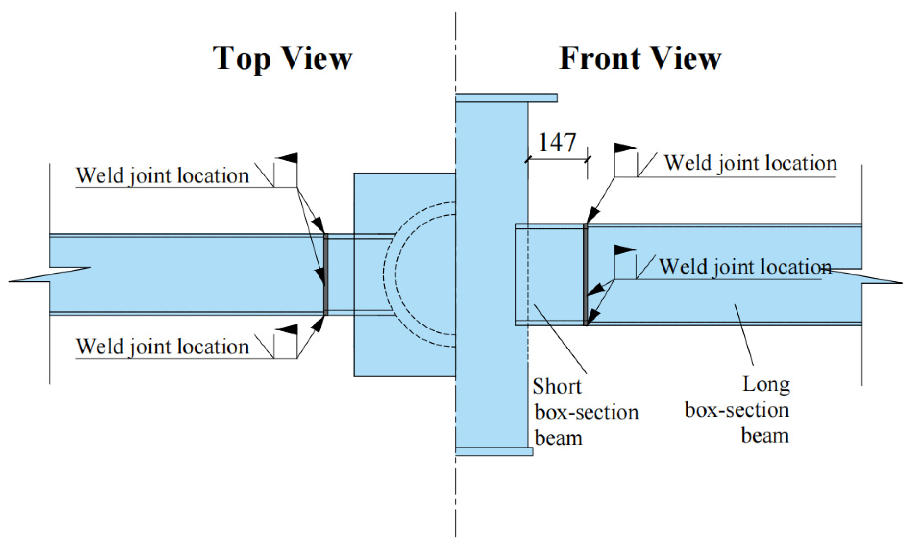
Based on a real-world prototype steel frame from Nanchang, China [17], a single-story beam-column substructure was extracted at a 1/3 scale from the inflection points of the bending moment, as shown in Figure 1. The side stub and the middle failure stub of the substructure were made of circular hollow steel sections with an external diameter of 356 mm and a thickness of 30 mm. The side stub had a length of 1230 mm. Short cantilever beams extending from both ends featured I-shaped cross-sections with a height of 250 mm and width of 200 mm; both the flanges and webs had a thickness of 12 mm. The internal main beam had a box-shaped cross-section with identical width and height and a clear span of 3250 mm. The purple rectangles in Figure 1 indicate the locations of the strain gauges. Additionally, the welded connection of the box beam was positioned near the beam-column joint, 147 mm from the edge of the stub, as shown in Figure 2. The flange thickness was 12 mm near the side stub and 8 mm near the middle stub.

Figure 1. Details of test steel frame substructure.

Figure 2. Details of weld connections of test substructure.

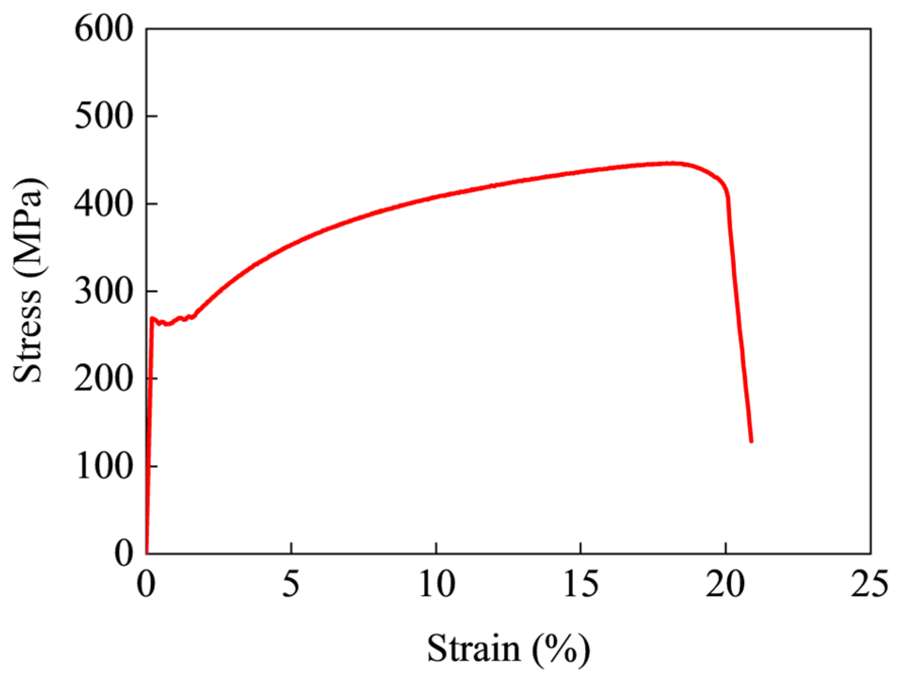
The base material was Grade Q235 structural steel according to the Chinese code GB50017-2017 [42], with a specified yield strength of 235 MPa. Uniaxial tensile tests determined the following material properties: an elastic modulus of 163,158 MPa, a yield strength f_y of 269 MPa, an ultimate strength f_u of 446 MPa, and a fracture elongation of 21%. The resulting stress–strain curve is shown in Figure 3.

Figure 3. Stress–strain curve of base material.

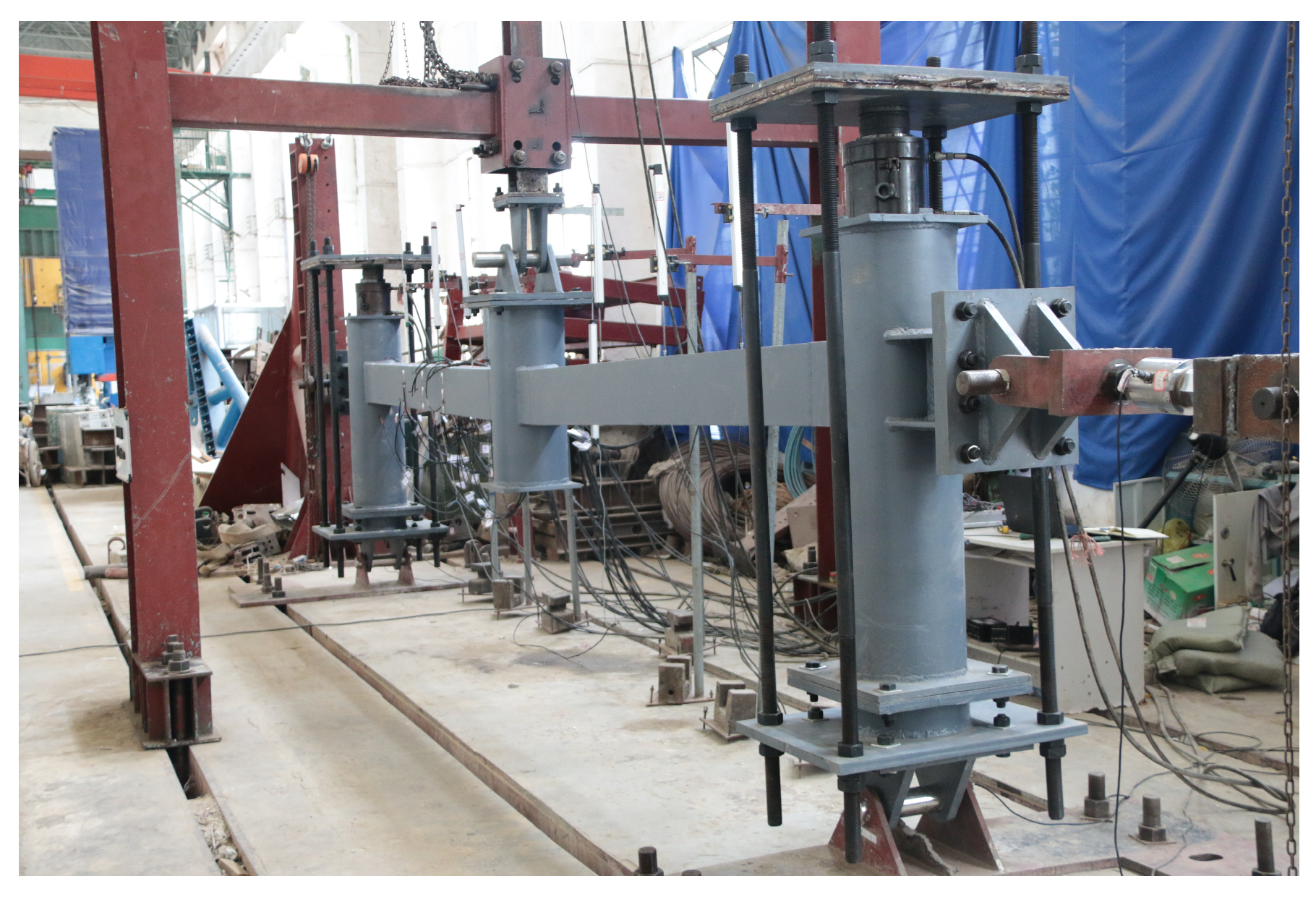
Quasi-static push-down tests were conducted on the specimen, as illustrated in Figure 4. The test setup followed the arrangement used by Qian [14], and consisted of a jack applying vertical displacement to the middle failure stub and an A-frame reaction system providing boundary restraint. Each side stub was bolted to a hinged support fixed to the ground, while the end plate of the cantilever beam was connected to the reaction support via a hinge, ensuring that no bending moments were transferred at the boundaries during loading. A self-balancing axial compression device was installed at the top of each side stub to maintain an axial compression ratio (ACR) of 0.3.

Figure 4. Test setup for push-down loading.

The specific axial compression force was determined by N = μf_cA_s, where μ is the ACR, f_c is the concrete compressive strength, and A_s is the area of the circular stub. The jack positioned atop the middle failure stub constrained the specimen to in-plane vertical displacement and rotation during loading. The load-carrying capacity of the substructure was measured using a load cell integrated into the jack, as illustrated in Figure 4.

2.2. Establishment of FEM

2.2.1. Model Overview

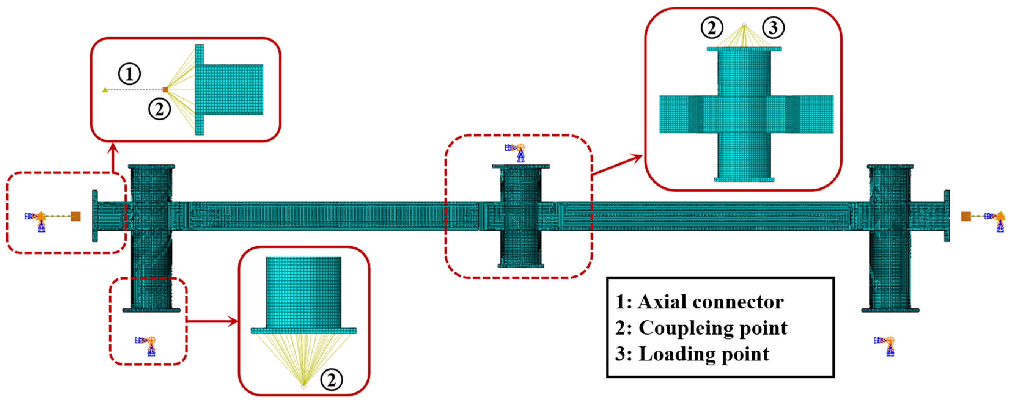
A finite element model (FEM) of the substructure was developed in ABAQUS 2021 following the specimen dimensions and test setup, as shown in Figure 5. The global mesh size was set to 15 mm using C3D8R elements. Notably, since premature failure was observed in the weld connection regions during testing, a weld-weakened zone was incorporated into the model. This zone extended 100 mm from the weld location and was discretized with a refined 5 mm mesh along the span direction. This modeling strategy effectively captures the performance degradation and stress concentration characteristics typical of the heat-affected zone in actual welded structures [43].

Figure 5. Establishment of FEM.

Regarding the boundary and loading conditions in FEM, the following simplifications were implemented: The top surface of the middle stub, the top and bottom surfaces of the side stubs, and the end plate surfaces of the cantilever beams were all coupled to a reference point. The reference point at the bottom of each side stub was constrained to allow only in-plane rotation. A concentrated axial force corresponding to an ACR of 0.3 was applied to the top reference points of the side stub. The reference point at the top of the middle stub was permitted in-plane vertical displacement and rotation. Based on experimental observations, a vertical displacement of 450 mm was applied at the top of the middle stub. Furthermore, the horizontal constraint provided by the link rod was simplified and modeled using a connector element with axial stiffness. Preliminary numerical analyses determined the axial stiffness of the connector was 17,200 kN/m.

The processed data from the uniaxial tensile tests described in Section 2.1 were incorporated into the ABAQUS material model using the “Plasticity” definition, with the material density specified as 7.85 × 10⁻⁶ kg/mm³. The input values for yield stress and plastic strain were derived from the test nominal stress–strain data, converted using Equations (1) and (2):

$${\sigma }_{\mathrm{T}}={\sigma }_{\mathrm{N}}(1+{\epsilon }_{\mathrm{N}})$$

(1)

$${\epsilon }_{\mathrm{T}}=\ln (1+{\epsilon }_{\mathrm{N}})$$

(2)

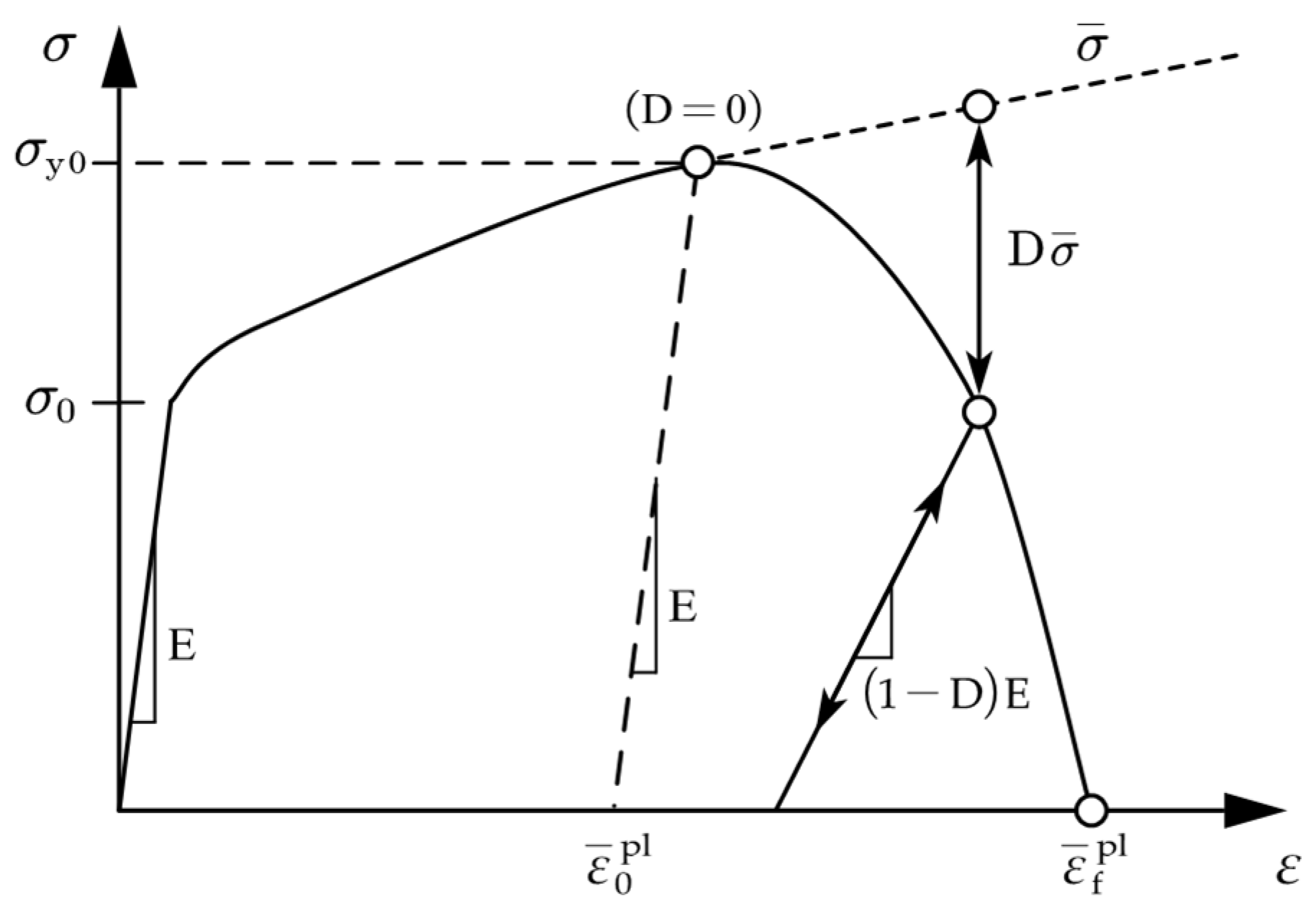
Here, ${\sigma }_{\mathrm{T}}$ and ${\sigma }_{\mathrm{N}}$ are the true stress and nominal stress (obtained from tests), respectively; ${\epsilon }_{\mathrm{T}}$ and ${\epsilon }_{\mathrm{N}}$ are the true strain and nominal strain. Ductile damage criteria for steel were additionally defined in ABAQUS to simulate the abrupt fracture behavior observed in weld joints, as illustrated in Figure 6. Where ${\stackrel{\mathrm{-}}{\epsilon }}_0^{\mathrm{pl}}$ is the equivalent plastic strain corresponding to the ultimate strength and the initial trigger of the damage, and ${\stackrel{\mathrm{-}}{\epsilon }}_{\mathrm{f}}^{\mathrm{pl}}$ represents the equivalent plastic strain at failure. The fracture energy G_F is the integral of the product of yield stress and characteristic length with respect to equivalent plastic strain over the range from ${\stackrel{\mathrm{-}}{\epsilon }}_0^{\mathrm{pl}}$ to ${\stackrel{\mathrm{-}}{\epsilon }}_{\mathrm{f}}^{\mathrm{pl}}$.

Figure 6. Ductile damage in ABAQUS.

In ABAQUS, the ductile damage requires definition of the fracture strain ${\stackrel{\mathrm{-}}{\epsilon }}_0^{\mathrm{pl}}$. Since the base material tests exhibited fracture immediately upon reaching the ultimate strength, the material was considered to possess low fracture energy. Accordingly, the failure strain ${\stackrel{\mathrm{-}}{\epsilon }}_0^{\mathrm{pl}}$ was defined as the true elongation of 0.19 for the base material, with the stress triaxiality and reference strain rate specified as 1/3 and 0, respectively.

Based on the findings of Jia [44], low-carbon steel exhibits significant reductions in yield strength, ultimate strength, and elongation under typical welding thermal conditions compared to the base metal. In FEM, this performance degradation in the weld-weakened zone was represented by applying a percentage reduction to the base material properties. This approach provides a macroscopic representation of the combined detrimental effects of weld defects and uncertainties on joint performance and progressive collapse resistance.

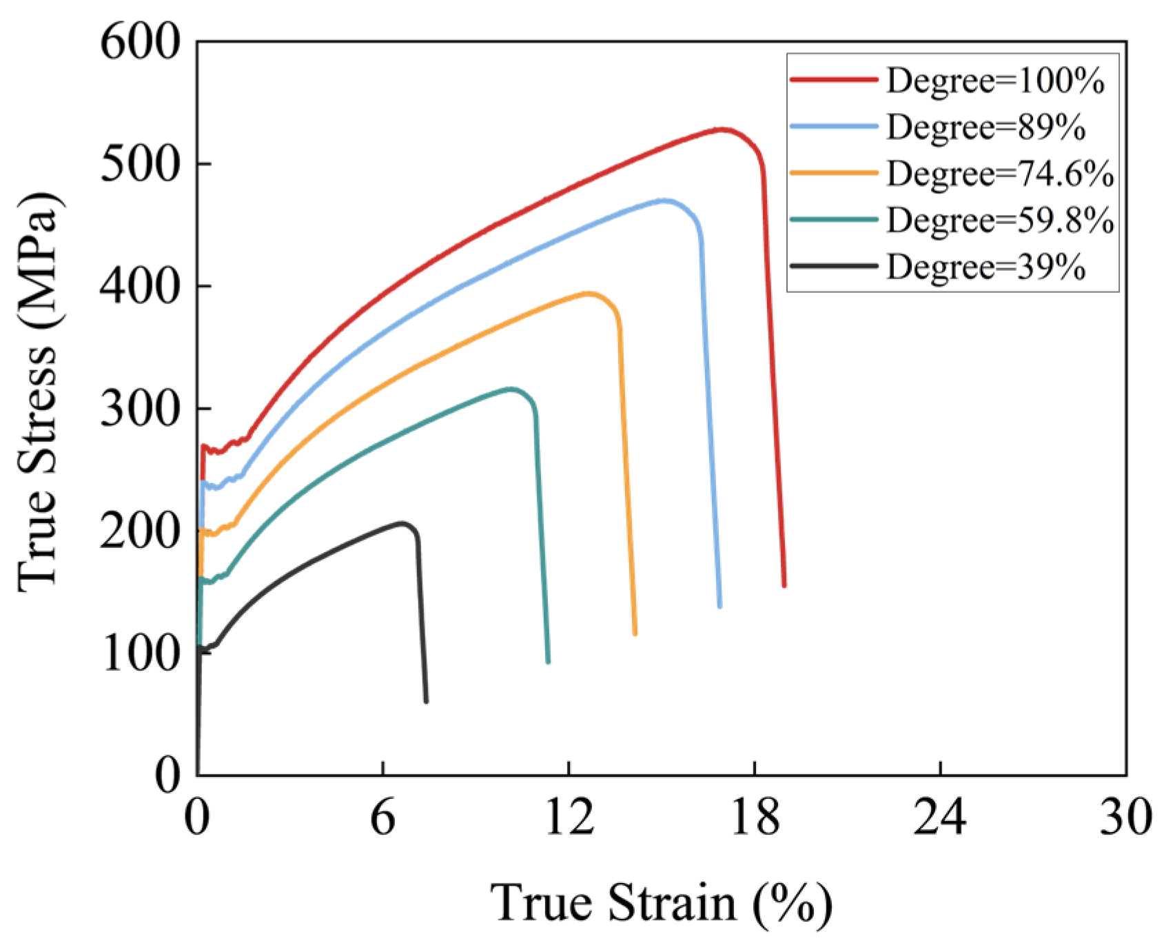
Based on the resistance development and failure modes observed in the push-down test, and considering that inferior weld quality can degrade structural performance by up to 50% [45], the following weakening degrees were applied to different locations within the weld-weakened zone: No reduction was applied to the weakened zones on the left main beam near either the side or middle stub. For the weakened zone on the right main beam near the middle stub, the bottom flange, top flange, and web were weakened to 39%, 89%, and 74.6% of the base material properties, respectively. For the weakened zone on the right main beam near the side stub, the bottom flange was unchanged, while the top flange and web were weakened to 59.8% and 74.6% of the base material properties, respectively.

These weakened degrees were determined through trail calculations to ensure the failure sequence in the weakened zone and the resistance development of the substructure at all loading stages accurately reflected the experimental behavior [17]. Figure 7 shows the true stress–strain curves under different weakened degrees, with the corresponding ductile damage parameters summarized in Table 1.

Figure 7. True stress–strain relationship under various reduction degrees.

Table 1. Ductile damage parameters under various reduction degrees.

Degree (%)	Fracture Strain (%)	Stress Triaxiality	Strain Rate (s−1)	Fracture Energy (N/mm2)
100	19	1/3	0	0.001
89	16.9	1/3	0	0.001
74.6	14.1	1/3	0	0.001
59.8	11.3	1/3	0	0.001
39	7.4	1/3	0	0.001

2.2.2. Model Validation

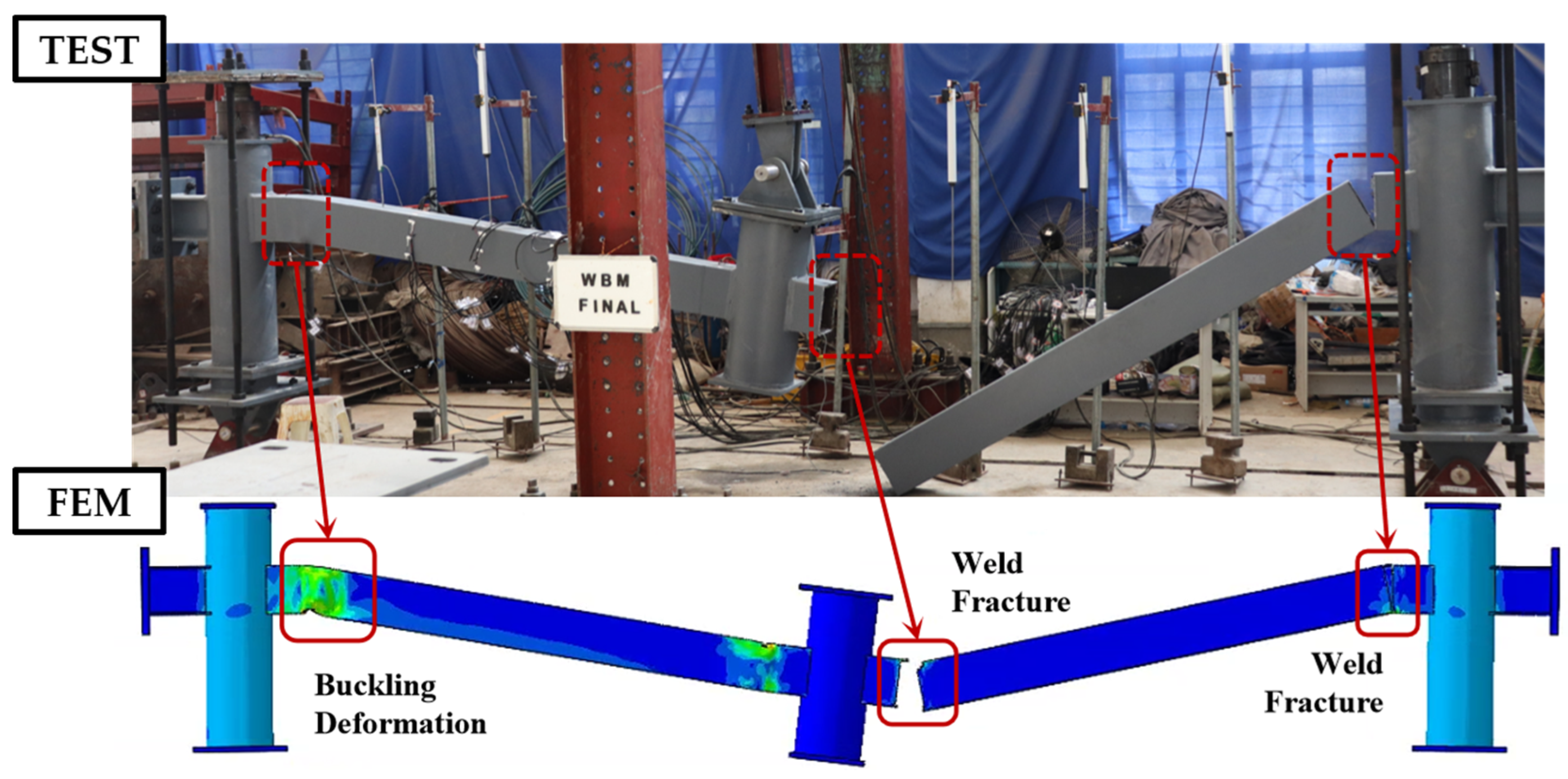
Figure 8 compares the failure modes obtained from FEM and tests. The results demonstrate that the incorporation of the weld-weakened zone in FEM successfully reproduces the joint failure observed in tests. Specifically, during the small deformation stage, the bottom flange in the weakened zone near the middle stub of the right main beam ruptured first. As the vertical displacement of the middle stub (MSD) increased, cracks propagated upward through the web toward the top flange. Concurrently, significant cracking developed at the top flange in the weakened zone near the side stub and progressed downward toward the bottom flange. Ultimately, at the final MSD, the weakened zone near the middle stub experienced complete fracture, indicating the total loss of the substructure’s resistance.

Figure 8. Comparison of failure modes between test and FEM.

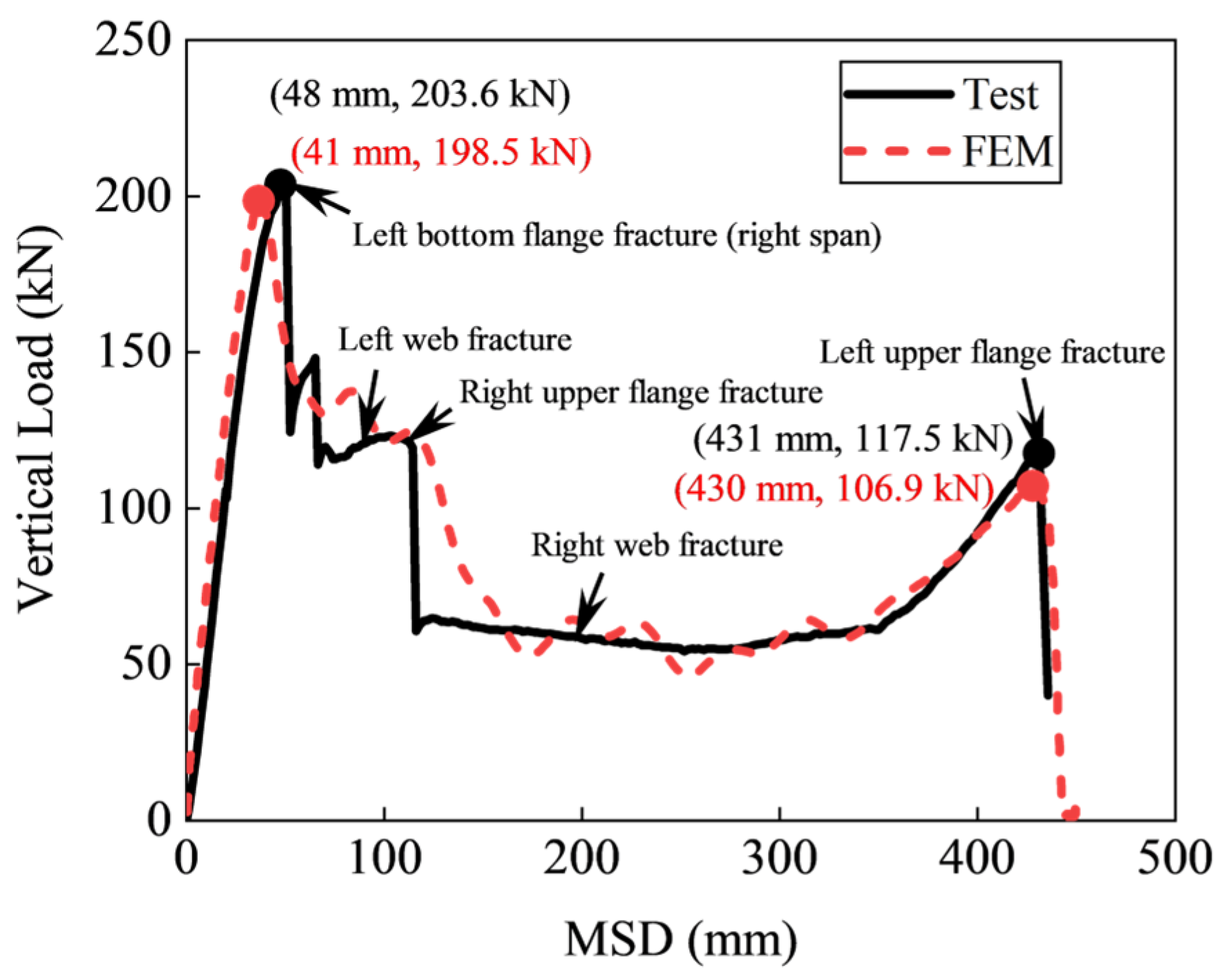
Figure 9 compares the vertical load versus middle stub displacement (MSD) curves obtained from the finite element analysis and experimental tests. The comparison reveals that due to the presence of weld defects, the development of vertical load in the substructure can be divided into three distinct phases. In the initial loading phase, the vertical load increases linearly with MSD, indicating elastic behavior dominated by frame action (FA). However, inconsistent weld quality led to fracture of the bottom flange in the weld-weakened zone near the middle stub of the right span. This fracture caused a sudden load drop when reaching the first peak load of 203.6 kN at an MSD of 48 mm.

Figure 9. Comparison of Load–MSD curves between test and FEM.

Subsequently, as the crack propagated upward through the web, the vertical load exhibited a brief plateau until fracture occurred in the top flange of the weakened zone near the side stub, resulting in a second load drop. Despite these localized failures, the maintained connectivity between the web and flange in the weakened zone allowed the resistance to continue increasing with MSD, demonstrating the development of catenary action (CA). Ultimately, when the top flange in the weakened zone near the middle stub fractured, the substructure reached its second peak load of 117.5 kN before complete loss of resistance, with the corresponding ultimate MSD reaching 431 mm.

2.2.3. Sensitivity Analysis

To further validate the finite element model, Figure 10 presents a sensitivity analysis examining the effects of the width of the weakened zone, the mesh size within it, and the boundary stiffness. The results indicate that as the zone width decreases from 100 mm to 20 mm, the load reaches the second peak more rapidly after the resistance plateau phase, accompanied by premature structural failure. This suggests that the fracture process in the web and top flange of the weakened zone near the middle stub becomes more transient. When the width is reduced to 10 mm, although the resistance plateau phase is delayed, the web in the weakened zone near the middle stub fractures simultaneously with the bottom flange, resulting in complete loss of catenary action development capability.

Figure 10. Sensitivity analysis of validated FEM: (a) Weld-weakened zone width; (b) Weakened zone mesh size; (c) Boundary stiffness.

The refined mesh demonstrates closer alignment with test results by reducing structural resistance during both the plateau phase and catenary action development. However, excessively refined mesh may lead to premature structural failure. Meanwhile, increased boundary stiffness (K_B) enabled earlier transition from the resistance plateau phase and enhanced structural stiffness during catenary action development, though this improvement is accompanied by premature failure of the substructure.

Furthermore, the analysis reveals that the first peak load remained stable across all sensitivity cases, demonstrating that the configuration of the weld-weakened zone and boundary stiffness have minimal influence on the initial yielding behavior of the substructure. Based on the sensitivity study, the optimal model configuration is determined to be a weakened zone width of 100 mm, a local mesh size of 5 mm, and a boundary stiffness of 17,200 kN/m, as this combination most accurately reproduces the test response.

3. Progressive Collapse Database Creation

3.1. Parametric Modelling Program

Building upon the validated FEM established in Section 2, this study develops an efficient automated modeling program for substructure parameterization. The program is developed around driving the ABAQUS kernel through Python 2.7 code, automating the complete workflow including parts creation, material property definition, assembly, boundary condition application, and mesh generation. This approach not only eliminates time-consuming manual modeling operations but also ensure model consistency while generating a comprehensive progressive collapse database that incorporates multiple engineering design features and accounts for weld-weakened degrees.

Based on their significant influence on the progressive collapse resistance of steel frame substructures, eight categories of design features were selected to constitute the parametric design space, as summarized in Table 2. The parameters included: SL, denoting the span length of the main beam; FT and WT, representing the thickness of the flange and web of the box-section beam, respectively; CLR, defined as the ratio of the cantilever I-beam length to the main beam span; JWL, indicating the relative position ratio of the weld center, considering locations near both the middle and side stubs; WWD, signifying the degree of weakening within the weld-affected zone, applied to the top flange, bottom flange, and web; STH, calculated as the span-to-height ratio of the main beam; HTW, representing the height-to-width ratio of the beam section; DTW, defined as the diameter-to-width ratio of the circular tubular stub; DTT, calculated as the diameter-to-thickness ratio of the steel tube; ACR, denoting the axial compression ratio; Stiffness, representing the axial stiffness of the boundary connector; and Scenario, which considered both middle-stub and side-stub failure cases. Given that the validation substructure features a box-section main beam, this cross-sectional profile is adopted for all beams in the parametric models.

Table 2. Key feature categories of progressive collapse resistance.

Feature Category	Unit	Maximum	Minimum
SL	mm	1625	4875
FT	mm	4	20
WT	mm	4	20
CLR	%	0.05	0.2
JWL	%	0.03	0.3
WWD	%	0.3	1
STH	%	10.8	26
HTW	%	1	1.5
DTW	%	1.28	2.28
DTT	%	5.93	35.6
ACR	%	0	0.5
Stiffness	kN/m	1720	1,720,000
Scenario	-	Middle Stub	Side Stub

FT comprises FT-C and FT-F, representing the flange thickness of the short beam between the weld location and the stub, and the flange thickness of the long beam between the two weld locations, respectively; WT comprises WT-C and WT-F, denoting the corresponding web thickness; JWL comprises JWL-CJ and JWL-MJ, representing the relative position ratio of the weld-weakened area center near the side stub and the middle stub, respectively; WWD includes WWD-LSFT, WWD-LSFB, WWD-LSW, WWD-LMFT, WWD-LMFB, WWD-LMW, WWD-RSFT, WWD-RSFB, WWD-RSW, WWD-RMFT, WWD-RMFB, WWD-RMW. These denote the weld-weakened degree for the upper, lower flanges, and web regions of the weld-weakened area near the side stub of the left span beam, the weld-weakened degree for the three regions of the weakened area near the middle stub of the left span beam, and the weld-weakened degree for the corresponding regions in the right span.

After expansion, a total of 27 features were used to parameterize the FEM and construct the sample database. Figure 11 shows the models under two different failure scenarios: Figure 11a presents the validated benchmark model, while Figure 11b illustrates the model obtained by changing only the failure scenario.

Figure 11. FEM of two failure scenarios: (a) Middle stub failure; (b) Side stub failure.

Additionally, a dedicated script was developed to automatically extract historical output results from ODB files—specifically the load–MSD curves for each substructure—and process them into load–displacement angle (P–θ) curves, thereby standardizing the dataset for machine learning training and testing. It should be noted that the GSA 2016 defines a displacement angle of 0.2 as the critical limit state in pushover analysis [4]. Therefore, a maximum displacement angle of 0.2 was selected for loading each model, which corresponds to applying a vertical displacement at 0.2 times the span length.

3.2. LHS Hypercube Sampling

Given the 27-dimensional feature space, traditional random sampling would require a prohibitively large sample size to avoid clustering or sparsity issues while ensuring uniform feature coverage, resulting in unacceptable computational costs. In contrast, both Monte Carlo [46] and Latin Hypercube Sampling (LHS) [39,40] provide effective strategies for exploring high-dimensional feature combinations. Among these, LHS was selected for its superior space-filling capability and sampling efficiency with limited samples. By ensuring all possible values within each input feature range were sampled with equal probability and without repetition, LHS avoided sample clustering and facilitated parameter interactions at minimal computational cost.

The LHS procedure was implemented as follows: For a feature space of dimension d, the range of each feature was divided into N non-overlapping intervals of equal probability. For each feature j (j = 1, 2, …, d), a random permutation π_j(i) of the interval indices {1, 2, …, N} was generated. The value π_j(i) denoted the selected interval index for the i-th sample point of the j-th feature. Subsequently, a random value u_ij was sampled from the uniform distribution U(0,1). The specific feature value for the i-th sample point was then calculated as follows:

$$x_{ij}={\displaystyle \frac{{\pi }_j(i)-u_{ij}}{N}}$$

(3)

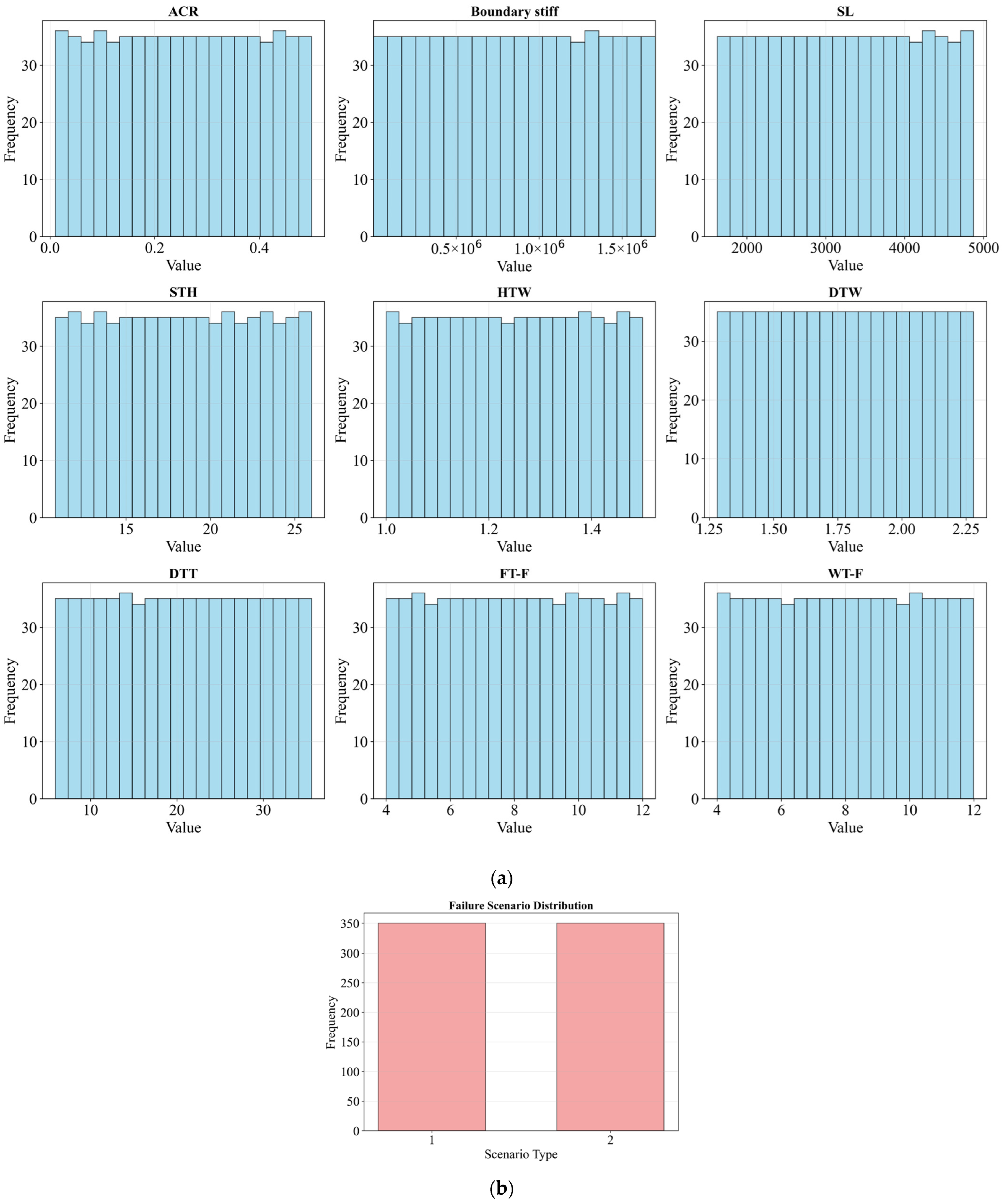
Assuming the first 26 features were uniformly distributed and the 27th feature was a discrete distribution (failure scenario), the sample size N was ultimately set to 700 after balancing computational cost and training accuracy.

Figure 12 presents the sampling distribution histograms for nine randomly selected continuous features and the failure scenario feature. The results show that the sample points were distributed approximately uniformly within each feature domain, with all intervals exhibiting comparable frequencies. Figure 13 shows the two-dimensional projection of samples for pairwise feature combinations, where the relatively uniform distribution of sampling points across all two-dimensional projections, without noticeable gaps or clustering patterns, confirmed the effectiveness of LHS in achieving comprehensive coverage of the high-dimensional parameter space. The random seed for the LHS process was set to 42 to ensure reproducibility.

Figure 12. Histogram of the distribution of features: (a) Random 9 features; (b) Feature of failure scenario.

Figure 13. LHS two-dimensional projection: (a) SL vs. STH; (b) ACR vs. Boundary stiffness; (c) HTW vs. DTW.

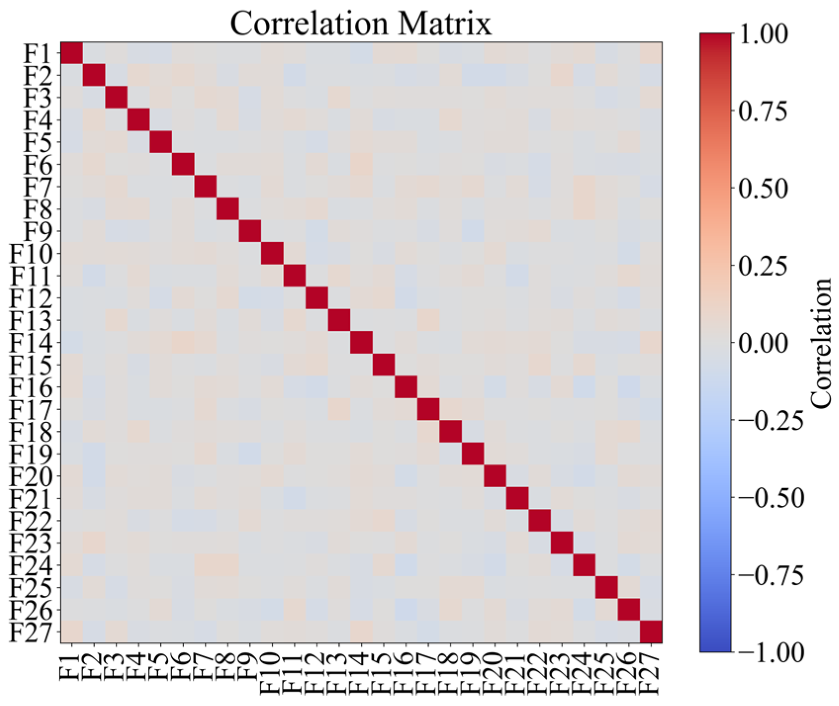
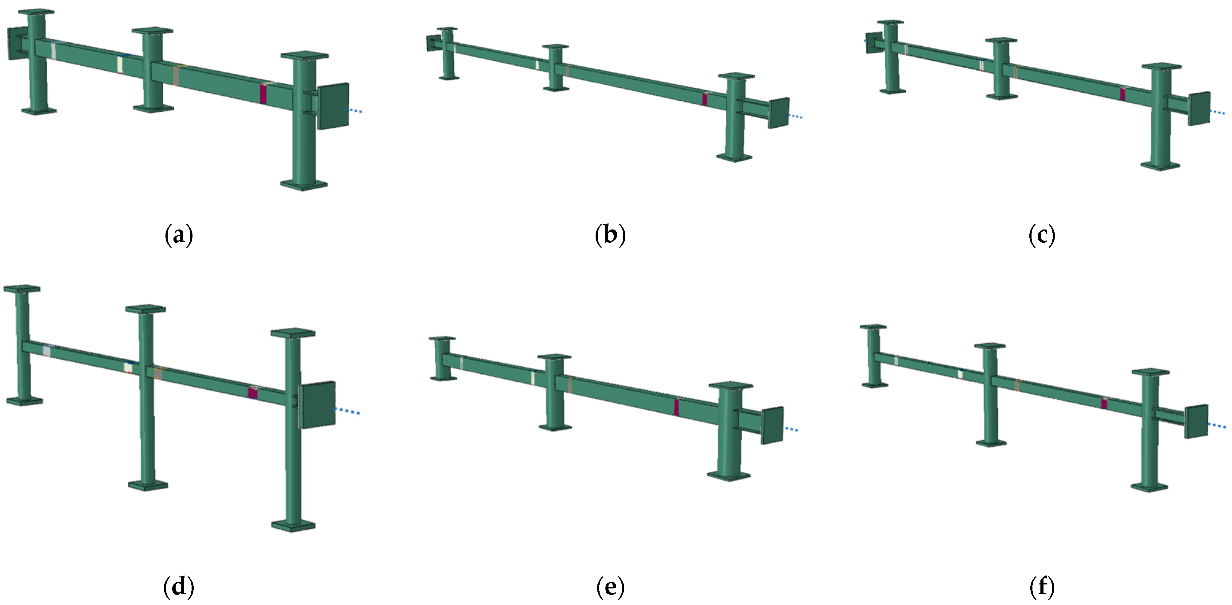
To further validate the independence of sampling points in the feature space, the correlation heatmap for all 27 features was shown in Figure 14. The absolute values of correlation coefficients between different features all remained below 0.2, confirming that the LHS method generated nearly independent or weakly correlated samples. This near-independence satisfies the requirement for input feature independence in machine learning training and contributes to enhanced model stability. Figure 15 displays six representative models randomly selected from the 700 samples, covering both failure scenarios.

Figure 14. Correlation matrix diagram of different features.

Figure 15. Parametric finite element modeling for substructure: (a) Sample 7; (b) Sample 351; (c) Sample 622; (d) Sample 158; (e) Sample 422; (f) Sample 669.

4. Machine Learning Prediction for Progressive Collapse Resistance

4.1. Machine Learning Frame

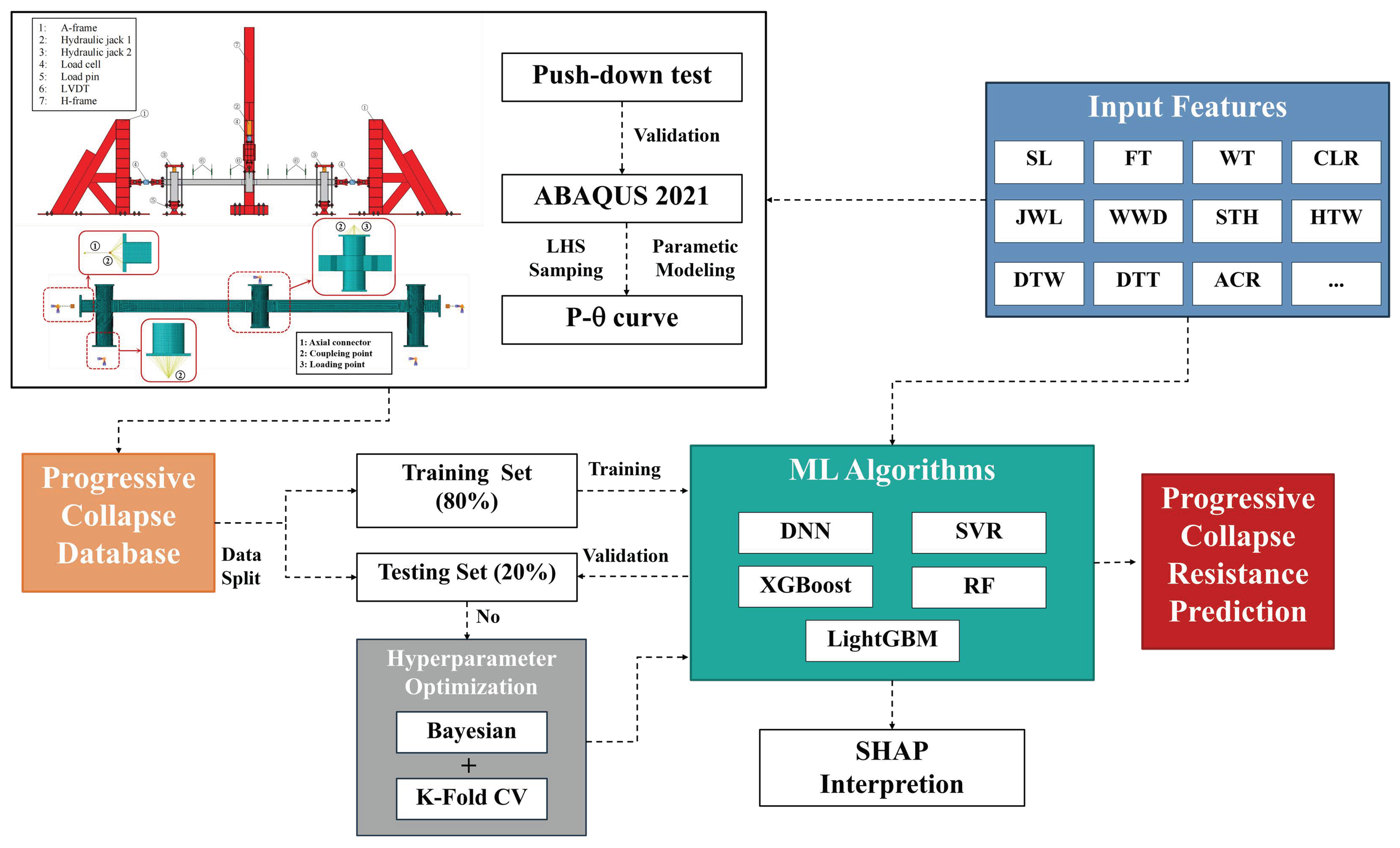
This section presents an ML framework for predicting the progressive collapse resistance of steel frame substructures with weld uncertainties, employing five distinct ML algorithms as illustrated in Figure 16. The framework implementation began with the parameterized modeling program and LHS described in Section 2, which efficiently generated 700 FEMs with INP files covering different configurations across the 27 features. The complete P–θ curves served as outputs to establish the progressive collapse database.

Figure 16. Machine learning frame for progressive collapse resistance prediction.

Through the parametric modeling procedure on a 24-core parallel computing resource operating at 3.2 GHz base frequency, each substructure model required approximately 10–20 min from generation through computation to extraction of the P–θ sequence. The complete set of 700 models generally required about two weeks to generate the full database.

Simultaneously, five ML algorithms (DNN, SVR, RF, XGBoost, and LightGBM) were implemented to train the database. Given the critical importance of hyperparameter selection for model performance, a combined strategy of Bayesian optimization [47] and K-fold cross-validation [48] was employed to ensure robust training outcomes through careful tuning and validation. The optimal algorithm was selected based on its predictive accuracy and overall performance. SHAP analysis [41] was then applied to the best-performing model to quantitatively assess the contribution of each input feature to the predictions, thereby enhancing the interpretability and physical relevance of the ML results.

4.2. Machine Learning Algorithms

4.2.1. Deep Neutral Network (DNN)

The Deep Neural Network (DNN) represents a complex artificial neural network architecture comprising multiple layers of interconnected neurons. Each neuron receives inputs, performs nonlinear transformation through activation functions, and generates outputs. The key characteristic of DNNs lies in their inclusion of multiple hidden layers, which enable the learning of complex functional mappings through cascaded nonlinear transformations, making them particularly suitable for high-dimensional nonlinear regression problems. In this study, the forward propagation process of the DNN is described by Equation (4):

$$a^{\left[l\right]}=\mathrm{ReLU}\left(Z^{\left[l\right]}\right)=\mathrm{ReLU}\left(W^{\left[l\right]}{a}^{\left[l-1\right]}+b^{\left[l\right]}\right)$$

(4)

${\mathit{a}}^{\left[l\right]}$ represents the output matrix of the l-th neuron layer, ${\mathit{Z}}^{\left[l\right]}$ is the corresponding input vector, ${\mathit{W}}^{\left[l\right]}$ and ${\mathit{b}}^{\left[l\right]}$ are the weight matrix and the bias vector of that layer, respectively. ReLU is the nonlinear activation function described as

$$\mathrm{ReLU}\left(z\right)=\max \left(0,z\right)$$

(5)

For the backpropagation process of the DNN, the mean squared error (MSE) served as the loss function, as specified in Equation (6).

$$\mathcal{L}\left(W,b\right)={\displaystyle \frac{1}{m}}{\displaystyle \sum _{i=1}^m\frac{1}{2}}{‖{\widehat{y}}^{\left(i\right)}-y^{\left(i\right)}‖}_2^2$$

(6)

where m is the number of feature samples, ${\widehat{y}}^{\left(i\right)}$ and $y^{\left(i\right)}$ are vectors of predicted value and true value of the i-th sample, respectively. Therefore, the gradient δ of the output layer L and the hidden layer l can be calculated according to Equations (7) and (8):

$${\delta }^{\left[L\right]}={\displaystyle \frac{\partial \mathcal{L}}{\partial Z^{\left[L\right]}}}={\displaystyle \frac{\partial \mathcal{L}}{\partial A^{\left[L\right]}}}{\displaystyle \frac{\partial A^{\left[L\right]}}{\partial Z^{\left[L\right]}}}=\left(A^{\left[L\right]}-Y\right)\odot {\mathrm{ReLU}}^{\prime \left[L\right]}\left(Z^{\left[L\right]}\right)$$

(7)

$${\delta }^{\left[l\right]}={\displaystyle \frac{\partial \mathcal{L}}{\partial Z^{\left[l\right]}}}=\left({\left(W^{\left[l+1\right]}\right)}^{\mathrm{T}}{\delta }^{\left[l+1\right]}\right)\odot {\mathrm{ReLU}}^{\prime \left[l\right]}\left(Z^{\left[l\right]}\right)$$

(8)

where ${\mathit{A}}^{\left[L\right]}$ represents the activation output vector of the output layer, and Y denotes the true value matrix. For the weight matrix and the bias vector, the basic update after gradient descent is dependent on the hyperparameter learning rate α.

$$W^{\left[l\right]}\leftarrow W^{\left[l\right]}-\alpha {\displaystyle \frac{\partial \mathcal{L}}{\partial W^{\left[l\right]}}}$$

(9)

$$b^{\left[l\right]}\leftarrow b^{\left[l\right]}-\alpha {\displaystyle \frac{\partial \mathcal{L}}{\partial b^{\left[l\right]}}}$$

(10)

In this study, the weights and biases of the DNN were iteratively updated using the Adam optimizer. This optimizer adapts the learning rate for each parameter by estimating the first and second moments of the gradients, thereby accelerating convergence and enhancing training stability. The initial learning rate was determined through hyperparameter optimization.

4.2.2. Support Vector Regression (SVR)

Support Vector Regression (SVR) is a supervised learning method based on Support Vector Machines. It seeks an optimal hyperplane in a high-dimensional feature space that maximizes the margin while ensuring that most data points lie within an ϵ-insensitive band around the predicted values. This approach provides excellent generalization capability for regression tasks.

SVR utilizes a specialized ϵ-insensitive loss function that measures prediction errors by penalizing only those deviations exceeding the ϵ threshold. For a single-output system, the loss function is defined as

$$L_{ϵ}\left(y,\widehat{y}\right)=\left\{\begin{array}{cc}0& \mathrm{if}\hspace{0.17em}\left|y-\widehat{y}\right|\le ϵ\\ \left|y-\widehat{y}\right|-ϵ& \mathrm{otherwise}\end{array}\right.$$

(11)

This means that if the absolute difference between the predicted value $\widehat{y}$ and the true value y is within ϵ, the loss is 0. To account for samples falling outside the ϵ-insensitive margin, SVR introduces slack variables ${\xi }_i$ and ${\xi }_i^{*}$. The primal form of its optimization problem is as follows:

$$\underset{w,b,{\xi }_i,{\xi }_i^{\ast }}{\min }{\displaystyle \frac{1}{2}}{‖w‖}^2+C{\displaystyle \sum _{i=1}^m\left({\xi }_i+{\xi }_i^{\ast }\right)}$$

(12)

where ${\displaystyle \frac{1}{2}}{‖w‖}^2$ is the regularization term. Minimizing it meant finding a flatter hyperplane to prevent overfitting. C is the hyperparameter penalty coefficient; a larger value indicates a narrower margin. The two slack variables ${\xi }_i$ and ${\xi }_i^{*}$ quantify the error amounts above and below the margin for the i-th sample. By the Lagrange multiplier method, the above can be transformed into a dual form that is easier to solve:

$$\begin{array}{c}\underset{\alpha ,a^{\ast }}{\max }-{\displaystyle \frac{1}{2}}{\displaystyle \sum _{i=1}^m{\displaystyle \sum _{j=1}^m\left({\alpha }_i-{\alpha }_i^{\ast }\right)\left({\alpha }_j-{\alpha }_j^{\ast }\right)K\left(x_i,x_j\right)-ϵ{\displaystyle \sum _{i=1}^m\left({\alpha }_i+{\alpha }_i^{\ast }\right)+{\displaystyle \sum _{i=1}^m{y}_i\left({\alpha }_i-{\alpha }_i^{\ast }\right)}}}}\\ \mathrm{s}.\mathrm{t}.\hspace{0.17em}{\displaystyle \sum _{i=1}^m\left({\alpha }_i-{\alpha }_i^{\ast }\right)=0,\hspace{0.17em}\hspace{0.17em}0\le {\alpha }_i\le C,\hspace{0.17em}\hspace{0.17em}0\le \hspace{0.17em}\hspace{0.17em}}{\alpha }_i^{\ast }\le C,\hspace{0.17em}\hspace{0.17em}i=1,\dots ,m\hspace{0.17em}\end{array}$$

(13)

where ${\alpha }_i^{*}$ and ${\alpha }_j^{*}$ are Lagrange multipliers, and $K({\mathit{x}}_i,{\mathit{x}}_j)$ is the kernel function, defined as $K({\mathit{x}}_i,{\mathit{x}}_j)=\exp \left(-\gamma {‖{\mathit{x}}_i-{\mathit{x}}_j‖}^2\right)$. This directly affects the performance and the applicability of the SVR. In SVR, algorithm performance primarily depends on the hyperparameters C, ϵ, and γ, which were obtained through Bayesian optimization and K-fold CV tuning.

4.2.3. Random Forest

Random Forest is an ensemble learning method that performs regression tasks by constructing and aggregating multiple decision trees. The core principle involves generating bootstrap samples from the original training data through sampling with replacement. Each sample subset is used to train an individual decision tree, and the final prediction is obtained by averaging the outputs of all trees. During the training of each tree, the algorithm randomly selects a subset of features at each node and identifies the optimal splitting feature from this subset. This feature randomization strategy enhances diversity among the trees, improving predictive accuracy and reducing overfitting.

When performing node splitting, the objective is to find a feature j and a split point s that partition the subset D_N of the current node N into two subsets D_L (x_j $\le$ s) and D_R (x_j > s), ensuring the MSE_split(j, s) is minimized.

$${\mathrm{MSE}}_{\mathrm{split}}\left(j,s\right)={\displaystyle \frac{m_L}{m_N}}\mathrm{MSE}\left(D_L\right)+{\displaystyle \frac{m_R}{m_N}}\mathrm{MSE}\left(D_R\right)$$

(14)

$$D_L=\left\{\left(x,y\right)\in D_N\left|x_j\right.\le s\right\}$$

(15)

$$D_R=\left\{\left(x,y\right)\in D_N\left|x_j\right.>s\right\}$$

(16)

where $m_L$ and $m_R$ denote the sample sizes of the left and right split regions, respectively, while MSE(D_L) and MSE(D_R) represent the mean squared errors of the left and right split regions, respectively. The optimal split $\left(j^{*}, s^{*}\right)$ is the combination of j and s that minimizes the MSE_split, as indicated in Equation (17). In RF algorithms, hyperparameters include the number of estimators, the maximum number of features, the maximum tree depth, and the minimum number of samples per split.

$$\left(j^{\ast },s^{\ast }\right)=\underset{j,s}{\mathrm{argmin}}\hspace{0.17em}{\mathrm{MSE}}_{\mathrm{split}}\left(j,\hspace{0.17em}s\right)$$

(17)

4.2.4. eXtreme Gradient Boosting (XGBoost)

XGBoost is an ensemble learning method that sequentially constructs decision trees in an additive manner. Unlike parallel ensemble methods, each new tree is specifically trained to correct the residual errors of the previous trees in the sequence. The final prediction is obtained by aggregating the weighted predictions from all constituent trees through a weighted sum. Furthermore, XGBoost optimizes a well-defined objective function using gradient descent, making it particularly effective for learning complex nonlinear relationships in high-dimensional feature spaces.

$${\widehat{y}}_i^{\left(t\right)}={\displaystyle \sum _{k=1}^t{f}_k\left(x_i\right)}={\widehat{y}}_i^{\left(t-1\right)}+f_t\left(x_i\right)$$

(18)

As shown in Equation (18), the prediction results are the sum of all trees’ predictions after t iterations. Here, f_k denotes the decision of the k-th tree, and f_t is the decision of the final tree. For the objective function requiring optimization, it includes the loss function and regularization terms, as shown in Equation (19).

$$\mathcal{L}={\displaystyle \sum _{i=1}^{n}l\left(y_i,\hspace{0.17em}{\widehat{y}}_i^{\left(t-1\right)}+f_t\left(x_i\right)\right)}+{\displaystyle \sum _{k=1}^t\mathsf{\Omega }\left(f_k\right)}$$

(19)

The loss function l is defined as the MSE in regression, while the regularization definition related to three hyperparameters, as indicated in Equation (20).

$$\mathsf{\Omega }\left(f\right)=\gamma T+{\displaystyle \frac{1}{2}}\lambda {\displaystyle \sum _{j=1}^T{w}_j^2}$$

(20)

where T represents the number of nodes in the tree, γ denotes the penalty coefficient for controlling the number of nodes, and λ is the L2 regularization coefficient, all of which are hyperparameters, while w_j is the weight of the j-th node. To optimize the objective function, a quadratic Taylor expansion of the loss function is performed, resulting in the following Equation (21).

$$\mathcal{L}={\displaystyle \sum _{i=1}^n\left[g_i{f}_t\left(x_i\right)+\frac{1}{2}{h}_i{f}_t^2\left(x_i\right)\right]}+\mathsf{\Omega }\left(f_t\right)$$

(21)

Defined the sample geometry of leaf node j as $I_j = i|q\left({\mathit{x}}_i\right) = j$, where $q\left({\mathit{x}}_i\right)$ is the function mapping samples to the leaf node. Then the optimal leaf node weight and corresponding optimal objective function value are as follows:

$$w_j^{\ast }=-{\displaystyle \frac{{\displaystyle {\sum }_{i\in I_j}{g}_i}}{{\displaystyle {\sum }_{i\in I_j}{h}_i+\lambda }}}$$

(22)

$${\mathcal{L}}^{\ast }=-{\displaystyle \frac{1}{2}}{\displaystyle \sum _{j=1}^T\frac{{\left({\displaystyle {\sum }_{i\in I_j}{g}_i}\right)}^2}{{\displaystyle {\sum }_{i\in I_j}{h}_i+\lambda }}}+\gamma T$$

(23)

By incorporating regularization terms into its objective function, XGBoost effectively controls model complexity to prevent overfitting. However, the optimization process involves multiple hyperparameters—including the learning rate, maximum tree depth, minimum leaf weight, subsampling and feature selection ratios, L1 and L2 regularization coefficients, and the number of estimators—thereby demanding substantial computational resources for hyperparameter tuning and model training.

4.2.5. Light Gradient Boosting Machnie (LightGBM)

Both LightGBM and XGBoost are gradient-boosting frameworks based on decision trees, yet they differ significantly in their implementation approaches. LightGBM employs Gradient-based One-Side Sampling (GOSS), which prioritizes samples with larger gradients during splitting under the assumption that these contribute more substantially to information gain. This strategy enables the algorithm to approximate optimal split points using a significantly smaller subset of the original data. Additionally, LightGBM utilizes Exclusive Feature Bundling (EFB) to combine mutually exclusive features into single features, thereby reducing the feature space dimensionality and accelerating the training process while maintaining model accuracy.

For the split of a leaf node I, assuming it splits into the left subset I_L and the right subset I_R, the split gain is calculated as shown in Equation (24).

$${\mathcal{L}}_{\mathrm{Gain}}={\displaystyle \frac{1}{2}}\left[{\displaystyle \frac{{\left({\displaystyle {\sum }_{i\in I_L}{g}_i}\right)}^2}{{\displaystyle {\sum }_{i\in I_L}{h}_i+\lambda }}}+{\displaystyle \frac{{\left({\displaystyle {\sum }_{i\in I_R}{g}_i}\right)}^2}{{\displaystyle {\sum }_{i\in I_R}{h}_i+\lambda }}}-{\displaystyle \frac{{\left({\displaystyle {\sum }_{i\in I}{g}_i}\right)}^2}{{\displaystyle {\sum }_{i\in I}{h}_i+\lambda }}}\right]-\gamma$$

(24)

4.3. Model Predictions

The five ML algorithms described above (DNN, SVR, RF, XGBoost, and LightGBM) were trained using the database of full-process P–θ curves for steel frame substructures. Given the wide numerical range of the input features—for instance, boundary stiffness varying from 1700 to 1,700,000 kN/m and the axial compression ratio (ACR) ranging from 0 to 0.5—the feature space was standardized using a standard scaler before training all algorithms. The optimal hyperparameters for the five ML methods, obtained through Bayesian optimization with 30 iterations and 5-fold cross-validation, along with their search ranges, are summarized in Table 3.

Table 3. Hyperparameter optimization.

Algorithm	Hyperparameters Optimization
DNN	Activation: ReLu; Hidden layers: 5 (3~8); Units: 439 (128~512); Dropout_rate: 0.1713 (0.15~0.4); Learning_rate: 0.0026 (0.0005~0.005); Batch_size: 31 (16~32); Epochs: 46 (16~500)
SVR	C: 832.4594 (0.1~1000); Epsilon: 0.0221 (0.001~0.1); Gamma: 1.8191 (0.001~10); Kernel: RBF
RF	N_estimators: 245 (50~500); Max_depth: 31 (5~50); Min_samples_split: 2 (2~20); Min_samples_leaf: 1 (1~10); Max_features: 0.1 (0.1~1)
XGBoost	N_estimators: 498 (100~500); Max_depth: 9 (3~10); Learning_rate: 0.0889 (0.01~0.1); Subsample: 0.7732 (0.7~0.9); Colsample_bytree: 0.8623 (0.7~0.9); Reg_alpha: 0.2368 (0.1~1); Reg_lambda: 0.9742 (0.1~1); Min_child_weight: 9 (1~10)
LightGBM	N_estimators: 328 (100~500); Max_depth: 10 (3~10); Learning_rate: 0.1 (0.01~0.1); Num_leaves: 28 (20~100); Subsample: 0.7 (0.7~0.9); Colsample_bytree: 0.9 (0.7~0.9); Reg_alpha: 0.1 (0.1~1); Reg_lambda: 1 (0.1~1); Min_child_sample: 12 (5~20)

Four commonly used regression metrics were employed to evaluate algorithm performance: the root mean square error (RMSE), coefficient of determination (R²), mean absolute error (MAE), and symmetric mean absolute percentage error (sMAPE), as defined in Equations (25)–(28). Here, m is the sample size in train or test set; $y_i$ and ${\widehat{y}}_i$ are the true value and predicted value, respectively.

$$\mathrm{RMSE}=\sqrt{{\displaystyle \frac{1}{m}}{\displaystyle \sum _{i=1}^m{\left(y_i-{\widehat{y}}_i\right)}^2}}$$

(25)

$${\mathrm{R}}^2=1-{\displaystyle \frac{{\displaystyle \sum _{i=1}^m{\left(y_i-{\widehat{y}}_i\right)}^2}}{{\displaystyle \sum _{i=1}^m{\left(y_i-\overline{y}\right)}^2}}}$$

(26)

$$\mathrm{MAE}={\displaystyle \frac{1}{m}}{\displaystyle \sum _{i=1}^m\left|y_i-{\widehat{y}}_i\right|}$$

(27)

$$\mathrm{sMAPE}={\displaystyle \frac{100\%}{m}}{\displaystyle \sum _{i=1}^m\left|\frac{y_i-{\widehat{y}}_i}{\left|y_i\right|+\left|{\widehat{y}}_i\right|}\right|}$$

(28)

RMSE quantifies the absolute deviation between predicted and actual values, with lower values indicating higher predictive accuracy. R² measures the proportion of variance in the target variable explained by the model, where values approaching 1 represent better performance. Both MAE and sMAPE offer complementary perspectives on prediction errors, with sMAPE being particularly valuable for error assessment under low-load conditions.

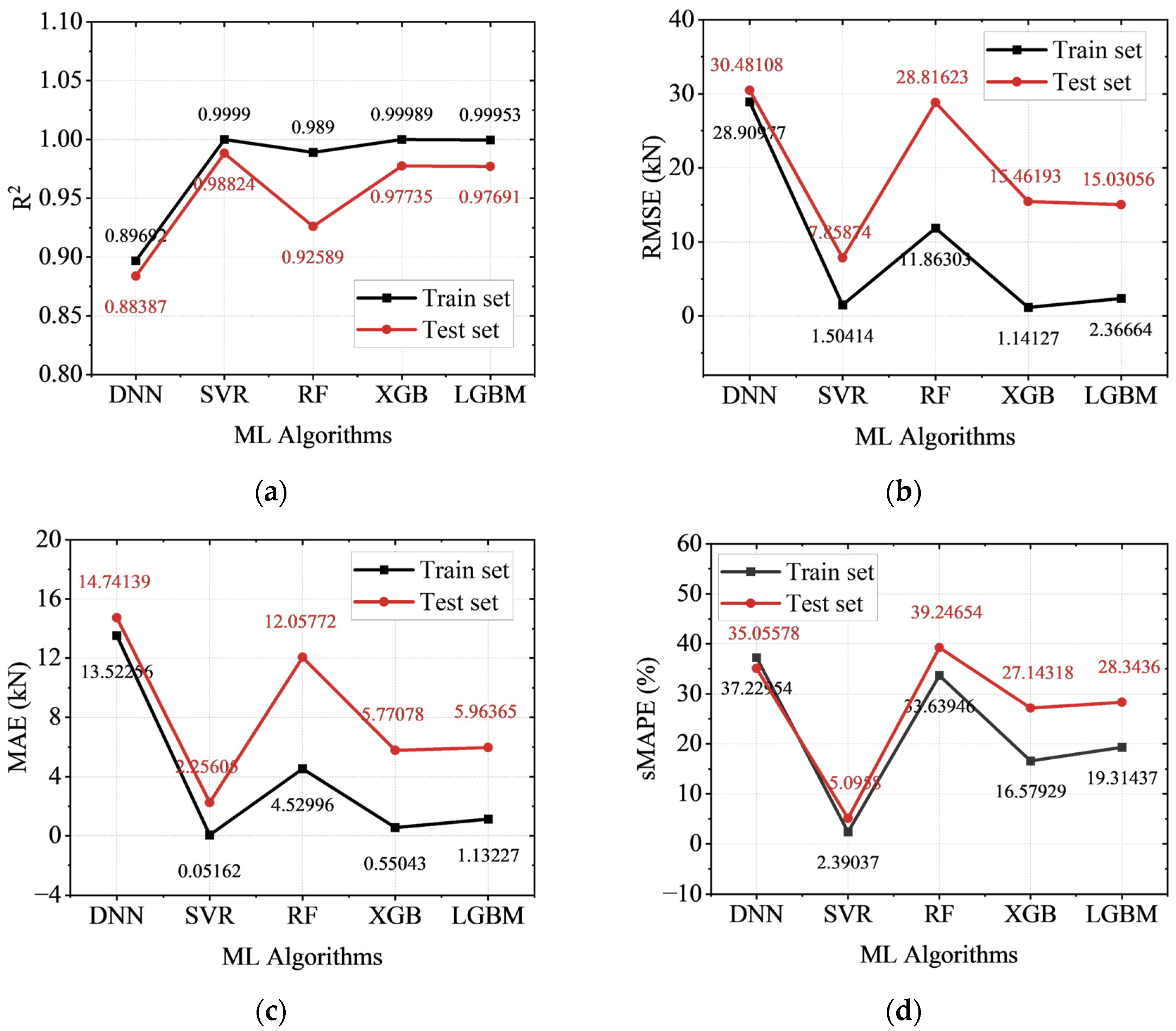
Figure 17 compares the performance of the five ML algorithms trained on the database. The results show that three of the algorithms—SVR, XGBoost, and LightGBM—achieved coefficients of determination exceeding 0.95 on both training and test sets, indicating their high predictive accuracy. Further error analysis revealed that SVR consistently achieved the lowest RMSE, MAE, and sMAPE values alongside the highest R² score on both datasets, demonstrating its superior predictive accuracy and generalization capability among all evaluated algorithms. In contrast, XGBoost and LightGBM showed noticeably degraded performance on the test set compared to the training set, suggesting potential overfitting. Both DNN and RF delivered suboptimal performance in this study, which can be attributed to the challenge of modeling high-dimensional feature relationships with limited training samples.

Figure 17. Performance of different ML algorithms: (a) R²; (b) RMSE; (c) MAE; (d) sMAPE.

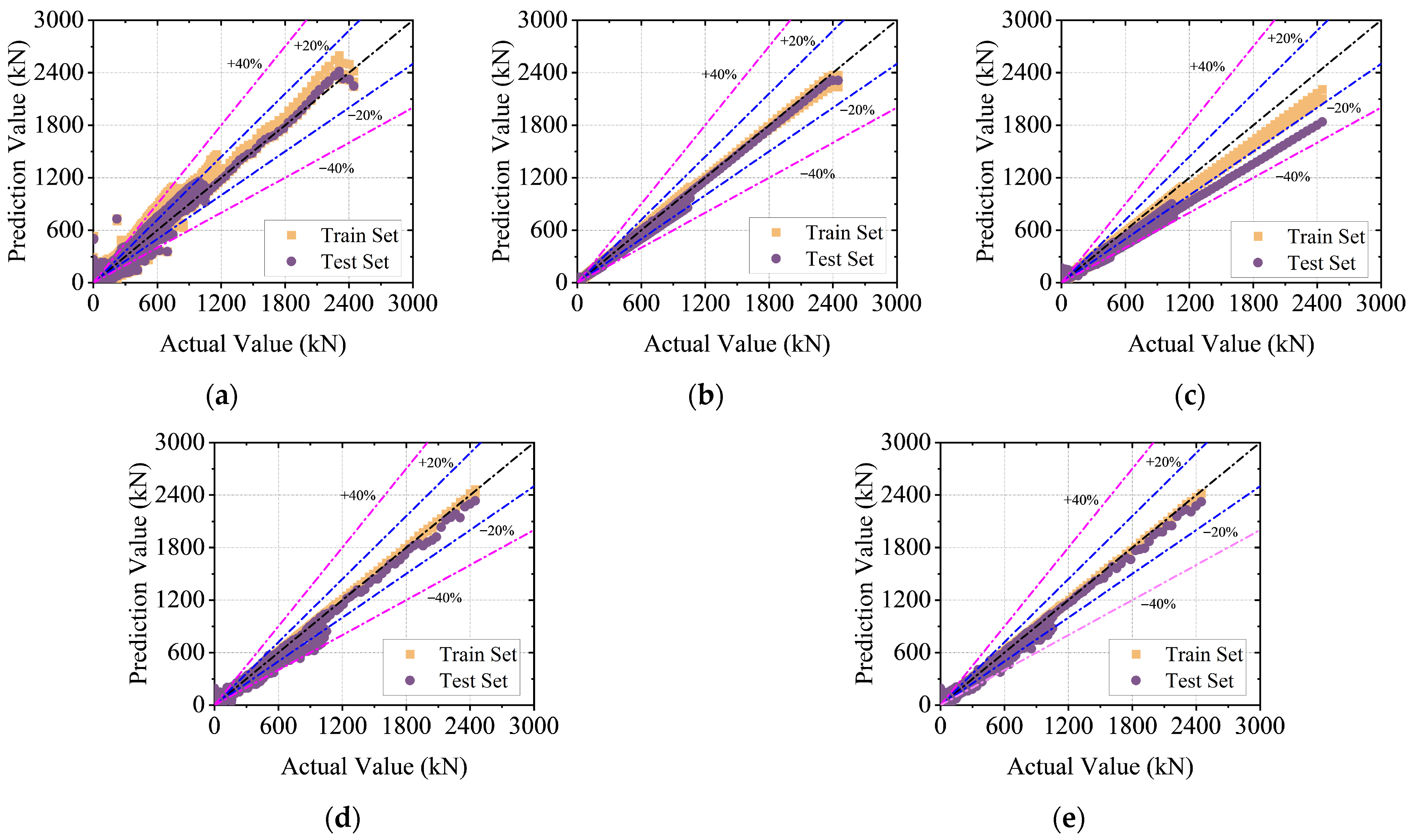
Figure 18 presents a comparison between the FEM results and the predicted load values from the five trained ML algorithms. It should be noted that the raw load-displacement curves obtained from FEM contained varying numbers of data points across different samples. To address this, each curve was first converted to P–θ format and then uniformly resampled to 50 points using linear interpolation through the Interp1d function from the SciPy library. This standardized interpolation approach effectively preserved the key characteristics of the original curves, including peak loads, as demonstrated by Figure 19. Consequently, each ML model’s training and prediction results shown in Figure 18 encompass 35,000 data points. Furthermore, to eliminate non-physical load oscillations near zero resistance, when the post-peak load in the interpolated P–θ curve dropped below zero, the structure was considered to have failed, and all subsequent load values were set to zero.

Figure 18. Prediction of loads of different machine learning algorithms: (a) DNN; (b) SVR; (c) RF; (d) XGBoost; (e) LightGBM.

Figure 19. Validation of data interpolation: (a) Sample 81; (b) Sample 274; (c) Sample 605.

Figure 18 reveals distinct performance patterns among the five ML algorithms. The prediction results of all algorithms except SVR showed substantial dispersion at lower load levels, while the RF algorithm exhibited significant prediction errors across the entire load range in the test set. In contrast, SVR maintained less than 20% deviation between predicted and actual loads on both training and test sets. DNN, XGBoost, and LightGBM demonstrated particularly large prediction errors for smaller loads in the test set, indicating their limited capability in capturing the structural response under low-load conditions.

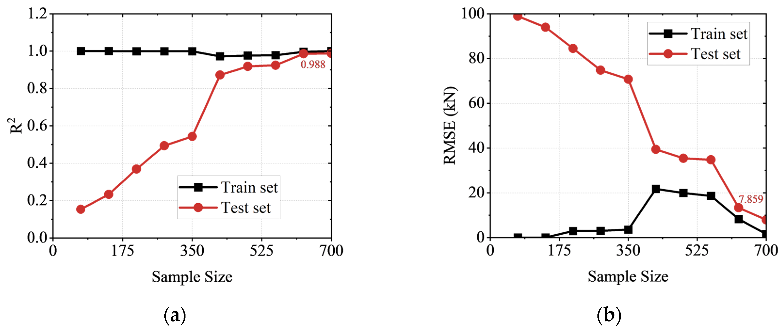
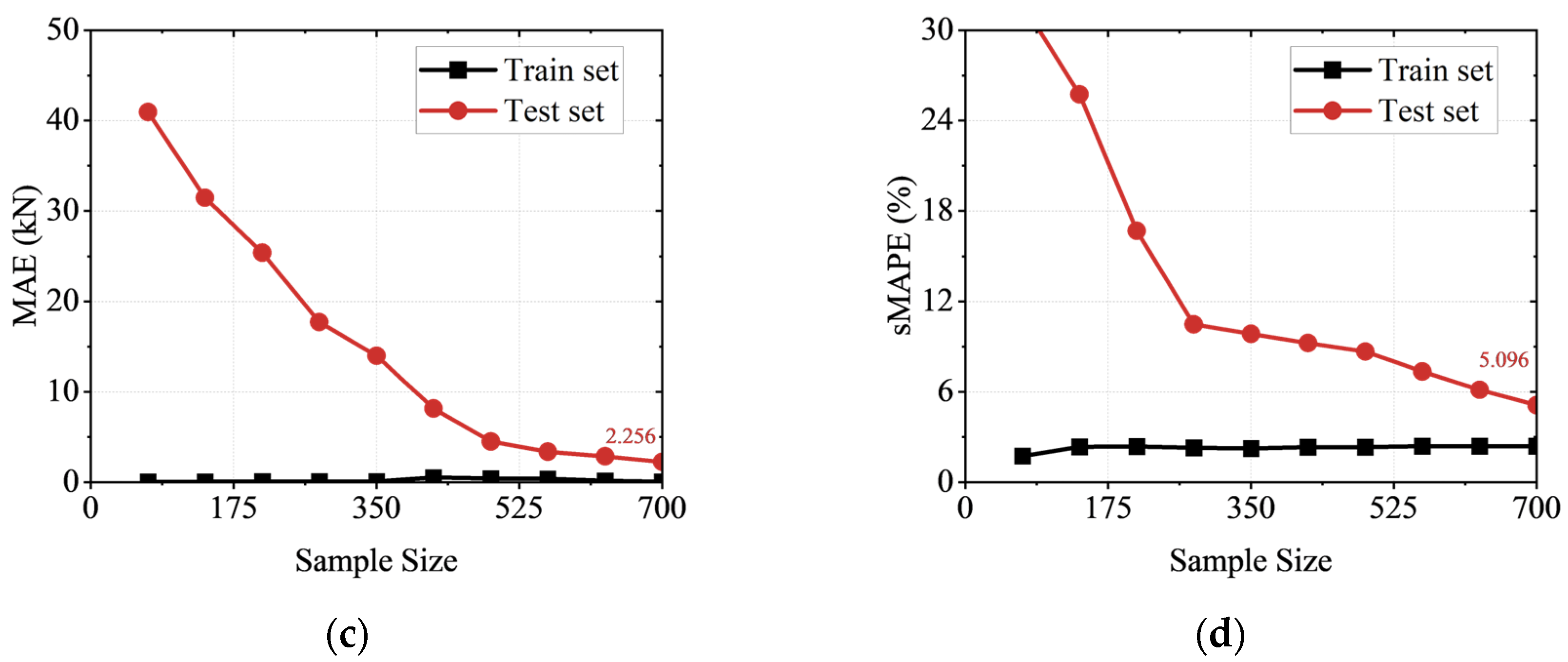
Figure 20 presents the learning curves for the SVR model, showing the relationship between training sample size and four performance metrics: R², RMSE, MAE, and sMAPE. The results demonstrate that as the sample size increases, all evaluation metrics on the test set progressively converge toward their corresponding training set values, indicating stabilized model performance and diminished generalization gap with sufficient data.

Figure 20. SVR learning curves: (a) R²; (b) RMSE; (c) MAE; (d) sMAPE.

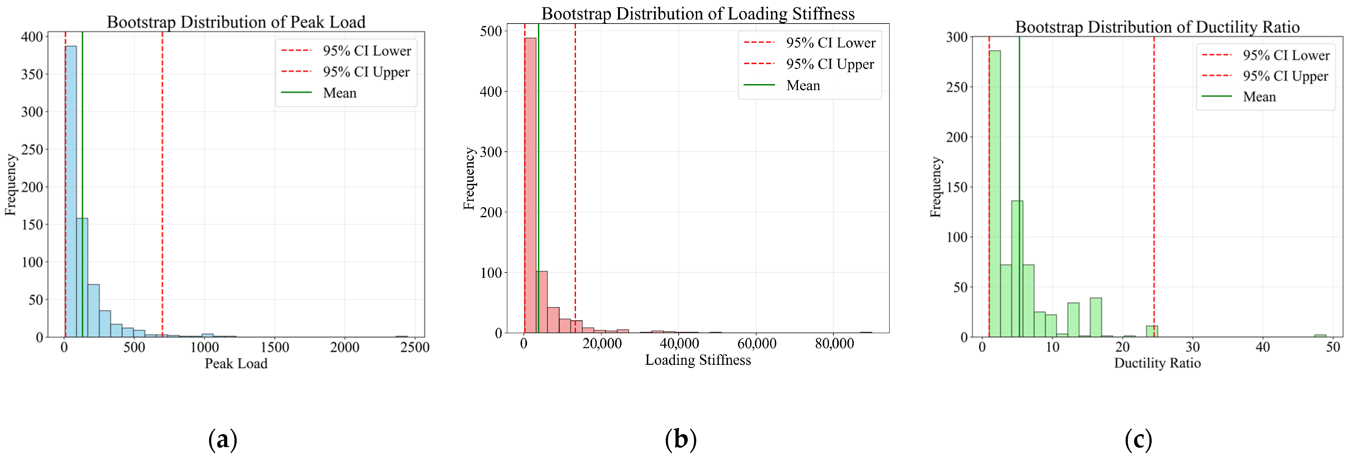
Considering there are three key indicators for comprehensively evaluating the progressive collapse resistance performance of substructures under the column removal: peak load P_max, loading stiffness K_e, and ductility ratio R_θ, which are expressed as Equations (29)–(31).

$$P_{\max }=\mathrm{Max}(P)$$

(29)

$$K_{\mathrm{e}}={\displaystyle \frac{P_{\mathrm{FP}}}{{\theta }_{\mathrm{FP}}}}$$

(30)

$$R_{\mathsf{\theta }}={\displaystyle \frac{{\theta }_{\mathrm{FP}}}{{\theta }_{\mathrm{Fail}}}}$$

(31)

where P_FP and θ_FP is the first peak load and the corresponding displacement angle, respectively, while θ_Fail is the displacement angle at failure. Therefore, based on the Bootstrap SVR, uncertainty analysis was subsequently performed for these three key indicators, with the results presented in Figure 21.

Figure 21. Uncertainty analysis based on Bootstrap SVR: (a) Peak Load; (b) Loading stiffness; (c) Ductility ratio.

As shown in Figure 21, the bootstrap distribution of the peak load follows a unimodal distribution with a mean value of approximately 130.86 kN and a 95% confidence interval ranging from 10.13 kN to 700.1 kN. The mean loading stiffness is 3793.53 kN/rad, with a 95% confidence interval of 280.56 kN/rad to 13,317.84 kN/rad. For the ductility ratio, the mean value is 5.3, with a 95% confidence interval spanning from 1 to 24.5. This substantial variability in structural performance during progressive collapse highlights the significant influence of factors such as weld quality and failure scenarios. The lower bound of the ductility ratio (approaching 1) indicates the potential for brittle failure modes, typically associated with fractures in joint welds. Consequently, ensuring high-quality welds in practice is crucial for maintaining adequate structural ductility and mitigating progressive collapse risks.

To further evaluate the importance of the Weld-Weakened Degree (WWD) features, an ablation study was conducted by removing them from the original SVR model. This removal resulted in the test set R² dropping to 0.923 and the sMAPE increasing from 5.096% to 14.281%. These results demonstrate that the WWD feature series is critical for maintaining the model’s prediction accuracy.

Figure 22 illustrates the hyperparameter tuning process for the SVR model using Bayesian optimization with 5-fold cross-validation. The optimized hyperparameters comprised C, ϵ, and γ. The optimization history reveals no clear correlation between individual hyperparameter values and the resulting R² scores (left y-axis) or MSE (right y-axis), which reflects the strength of the Bayesian approach: it selects hyperparameters based on both historical performance and uncertainty estimates from its probabilistic surrogate model, rather than through predetermined patterns. Compared to exhaustive methods like grid search, Bayesian optimization more efficiently explores the hyperparameter space to identify configurations approaching the global optimum, significantly improving training efficiency. With only three hyperparameters to tune, SVR required the least training time among the five ML algorithms, demonstrating a notable computational advantage for this application.

Figure 22. Optimal hyperparameters iteration history by Bayesian optimization and 5-Fold CV: (a) C; (b) Epsilon; (c) Gamma.

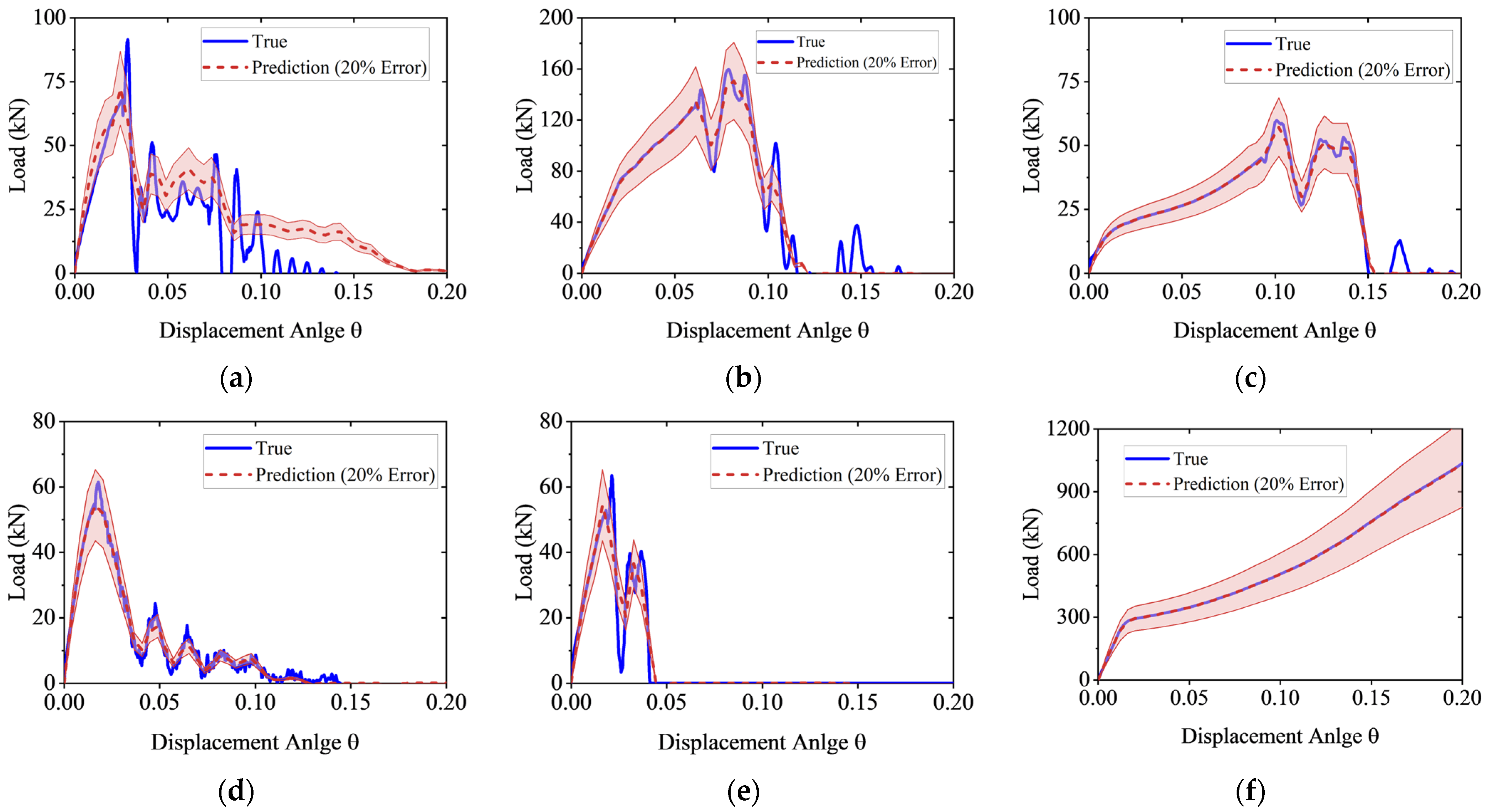
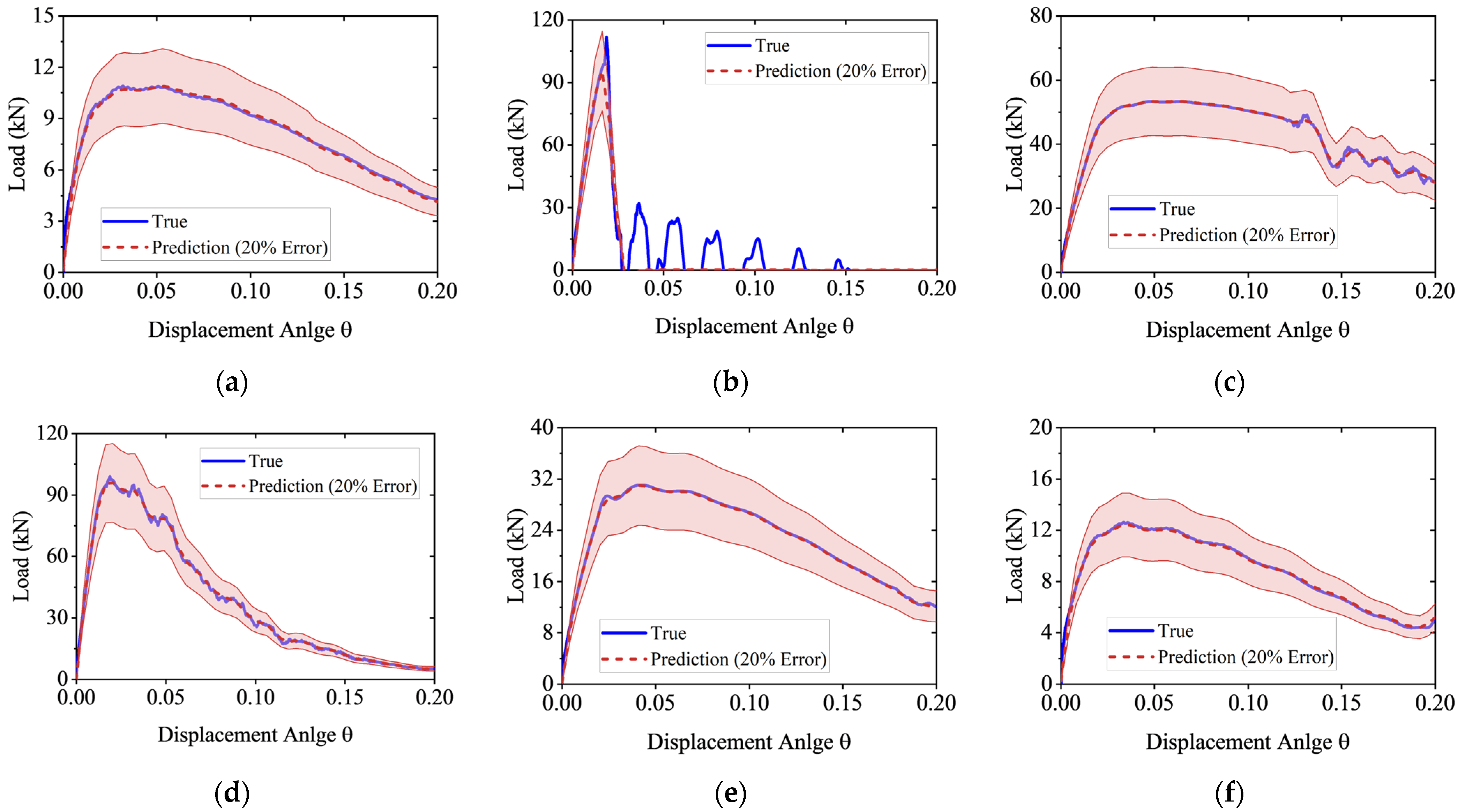
Figure 23 and Figure 24 compares the actual full-process P–θ curves with the predicted curves for 12 randomly selected samples from the SVR test set under two failure scenarios. It can be observed that the SVR prediction curves closely matched the actual results, effectively reflecting the development of the resistance of substructure under different combinations of features.

Figure 23. Full-process resistance prediction in test set by SVR (Middle stub failure): (a) Sample 4; (b) Sample 81; (c) Sample 163; (d) Sample 278; (e) Sample 452; (f) Sample 616.

Figure 24. Full-process resistance prediction in test set by SVR (Side stub failure): (a) Sample 13; (b) Sample 153; (c) Sample 274; (d) Sample 405; (e) Sample 581; (f) Sample 646.

To further validate the effectiveness of the SVR algorithm, Figure 25 compares the ML predictions with calculated results from Huang’s simplified mechanical model [21]. The analysis uses the validated substructure from [17], though Huang’s model did not account for weld uncertainty.

Figure 25. Verification of the predictions based on the theoretical model: (a) WWD boundary results [21]; (b) STH boundary results [21]; (c) Weld variability analysis [17].

Figure 25a presents the analysis of the test substructure without weld defects, where all material properties in the weakened zone remain at 100% of their base values. The theoretical results from Huang’s model remain within a 20% margin of the SVR predictions, demonstrating good agreement between both methods for the ideal weld condition. Figure 25b extends the validation by extrapolating the beam span-to-height ratio (STH) to the boundary of the feature domain, where the SVR prediction maintains accurate alignment with the theoretical curve, confirming the robust generalization capability. Figure 25c illustrates the sensitivity to weld quality through a comparative analysis where all weld-weakened degrees are set to 30% (blue curve). The area between this degraded response and the baseline curve (red) quantitatively represents the variability in progressive collapse resistance resulting from weld uncertainty, highlighting the significant influence of weld defects on structural performance. Compared to theoretical models, ML method not only enables efficient prediction but also accounts for the crucial effect of weld uncertainty on resistance, thereby offering broader applicability.

5. Machine Learning Interpretations

This section applies the SHAP (SHapley Additive exPlanations) method [41] to interpret the trained SVR model, aiming to reveal the effects and interactions of various features on the progressive collapse resistance of steel frame substructures. The insights derived from this interpretation provide the basis for developing practical design recommendations applicable to engineering practice.

SHAP is an interpretation method based on cooperative game theory that explains predictions from ML algorithms. Its core concept treats each feature as a participant in a cooperative game, with the final prediction representing the outcome of their collective contribution. The SHAP value ${\varphi }_i$ quantifies the marginal contribution of the i-th feature to the prediction. For a feature vector X of a given sample, the prediction $\widehat{f}\left(\mathit{X}\right)$ can be expressed as

$$\widehat{f}\left(X\right)={\varphi }_0+{\displaystyle \sum _{i=1}^M{\varphi }_i\left(X\right)}$$

(32)

where ${\varphi }_0$ represents the mean of all train set predictions, M denotes the number of features, and ${\varphi }_i$ is the SHAP value for the i-th feature. ${\varphi }_i$ > 0 indicates a positive contribution of that feature to the prediction; conversely, a negative value signifies the negative contribution. It should be noted that since the entire P–θ curve cannot be subjected to SHAP analysis, only peak load P_max, loading stiffness K_e, and ductility ratio R_θ are selected as the key indicators for SHAP analysis. All 700 samples were used for SHAP analysis.

5.1. Individual Interpretation

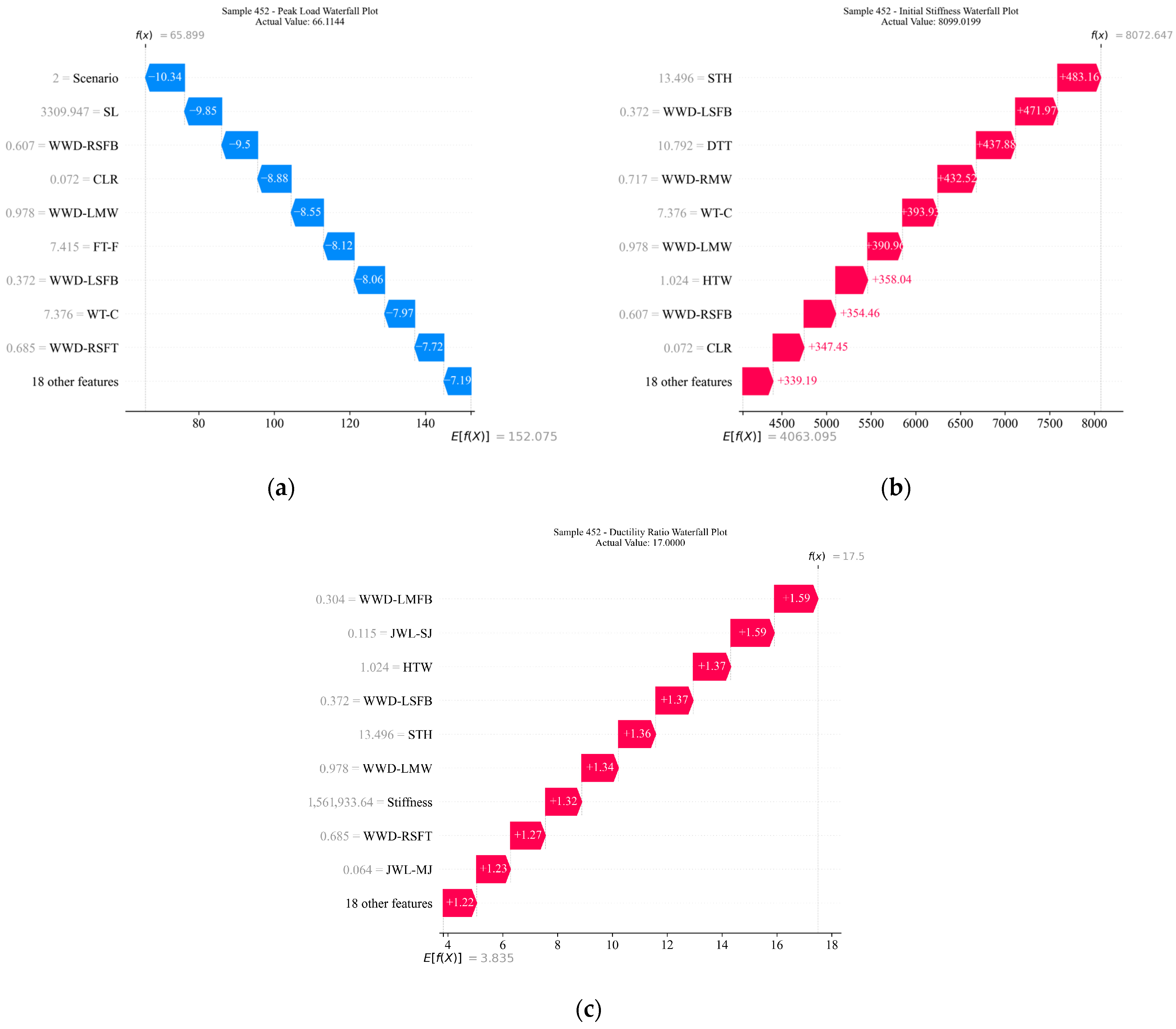
Figure 26 presents the SHAP waterfall plots for the peak load, loading stiffness, and ductility ratio corresponding to sample 452. The horizontal axis indicates the SHAP values, while the vertical axis lists the feature values for this specific sample. Features shown in blue exerted a negative influence on the prediction, whereas those in red had a positive effect. The baseline value E[f(X)] at the bottom corresponds to the expected model output ${\varphi }_0$. For the peak load prediction, the side stub failure scenario contributed −10.34 kN, the beam span length (SL = 3309.947 mm) contributed −9.85 kN, and the cantilever-to-span ratio (CLR = 0.072) contributed −8.88 kN. Notably, the combined negative contribution from the various weld-weakened degree (WWD) features across different locations totaled approximately −33.9 kN, establishing weld defects as the most significant detrimental factor affecting the substructure’s peak load.

Figure 26. SHAP waterfall plot for Sample 452: (a) Peak load; (b) Loading stiffness; (c) Ductility ratio.

For the loading stiffness K_e, the WWD feature series remained the dominant influencing factor, collectively accounting for approximately 1649.9 kN/rad. The beam span-to-height ratio (STH = 13.496) was the second most significant contributor, exerting an influence of 483.16 kN/rad. Subsequently, the stub diameter-to-thickness ratio (DTT = 10.792), the web thickness of the short beam segment between the weld location and the stub (WT-C = 7.376 mm), and the beam height-to-width ratio (HTW = 1.024) contributed 437.88 kN/rad, 393.93 kN/rad, and 358.04 kN/rad to the loading stiffness, respectively. In contrast to its effect on peak load, the failure scenario exerted limited influence on the loading stiffness.

For the ductility ratio R_q, consistent with the trends observed for peak load and loading stiffness, the WWD feature series remained the most influential factor, with a combined negative contribution of approximately −5.57. Other notable features included the relative position ratio of the weld location to the side stub (JWL–SJ = 0.115), contributing +1.59, the beam height-to-width ratio (HTW = 1.024) at +1.37, and the beam span-to-height ratio (STH = 13.496) at +1.36. Additionally, boundary stiffness (Stiffness = 1,561,933.64 kN/m) and the relative position ratio of the weld location to the middle stub (JWL–MJ = 0.115) positively influenced ductility, contributing +1.32 and +1.23, respectively.

5.2. Global Interpretation

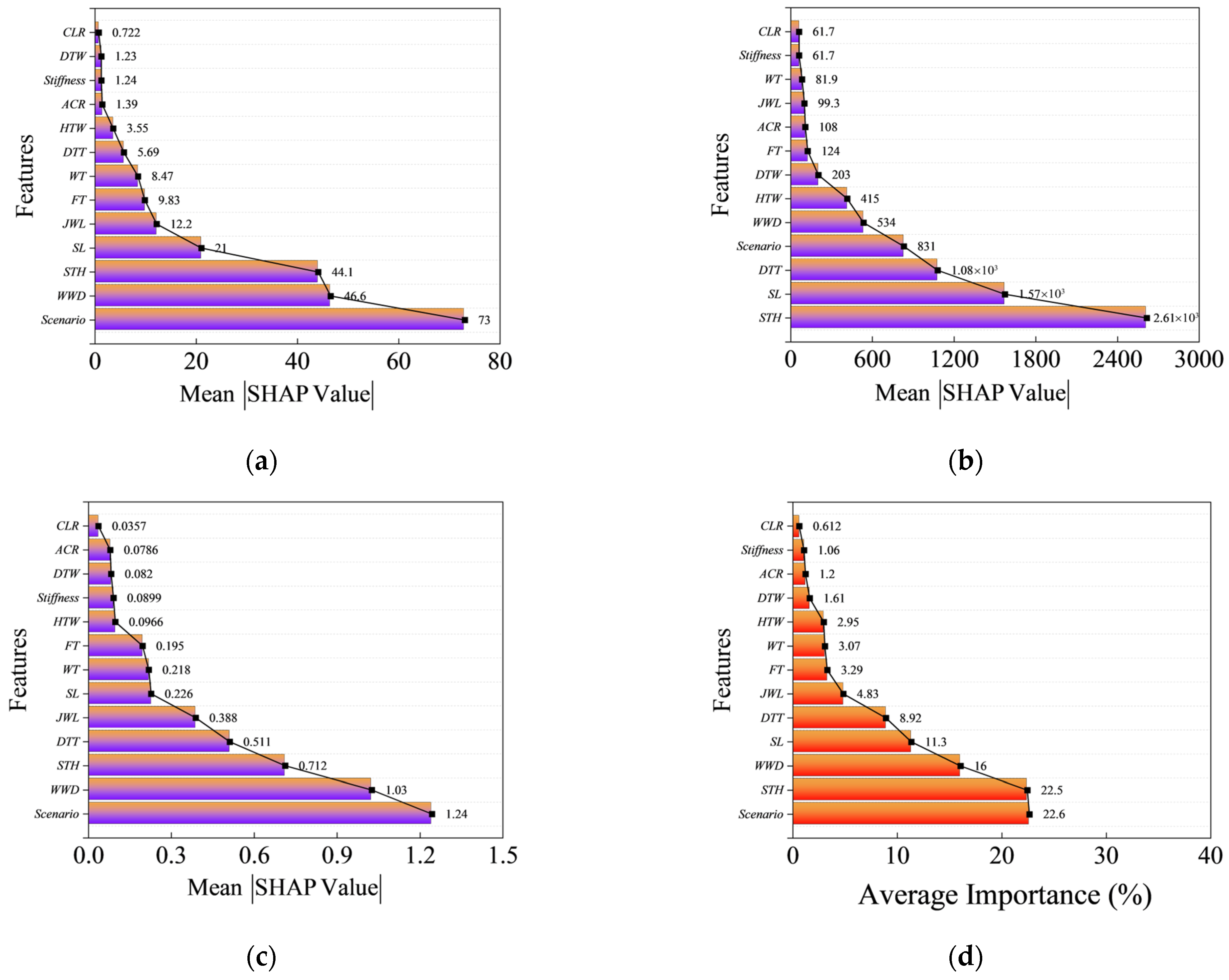
Based on the mean absolute SHAP values computed across all samples, Figure 27 presents the key features influencing the peak load, loading stiffness, and ductility ratio of steel frame substructures, along with their relative importance rankings. For clarity in interpretation, features of the same category have been aggregated—such as the various weld-weakened degree (WWD) features, which are grouped to represent their collective impact on structural performance.

Figure 27. SHAP global feature importance analysis: (a) Peak load; (b) Loading stiffness; (c) Ductility ratio; (d) Relative importance.

The results indicate that the failure scenario was the primary factor influencing the peak load and ductility ratio, while the weld defect (WWD) ranked among the top three critical factors. Therefore, ensuring weld quality should be prioritized in practical engineering applications. Additionally, for the peak load, the beam span-to-height ratio (STH), span length (SL), weld joint relative position ratio (JWL), beam web thickness (WT), and flange thickness (FT) also exerts significant influence. In terms of loading stiffness, the influence of STH is most pronounced, while the stub diameter-to-thickness ratio (DTT) is also critical, ranking third. For the ductility ratio, the influence of the DTT and JWL is more pronounced. By normalizing and averaging the feature rankings across these three aspects, an average importance ranking for the progressive collapse resistance of steel frame substructures is obtained, as shown in Figure 27d. The order is Scenario, STH, WWD, SL, DTT, JWL, FT, WT, HTW, DTW, ACR, Stiffness, and CLR. The corresponding importance values were 22.6%, 22.5%, 16%, 11.3%, 8.92%, 4.83%, 3.29%, 3.07%, 2.95%, 1.61%, 1.2%, 1.06%, and 0.612%, respectively.

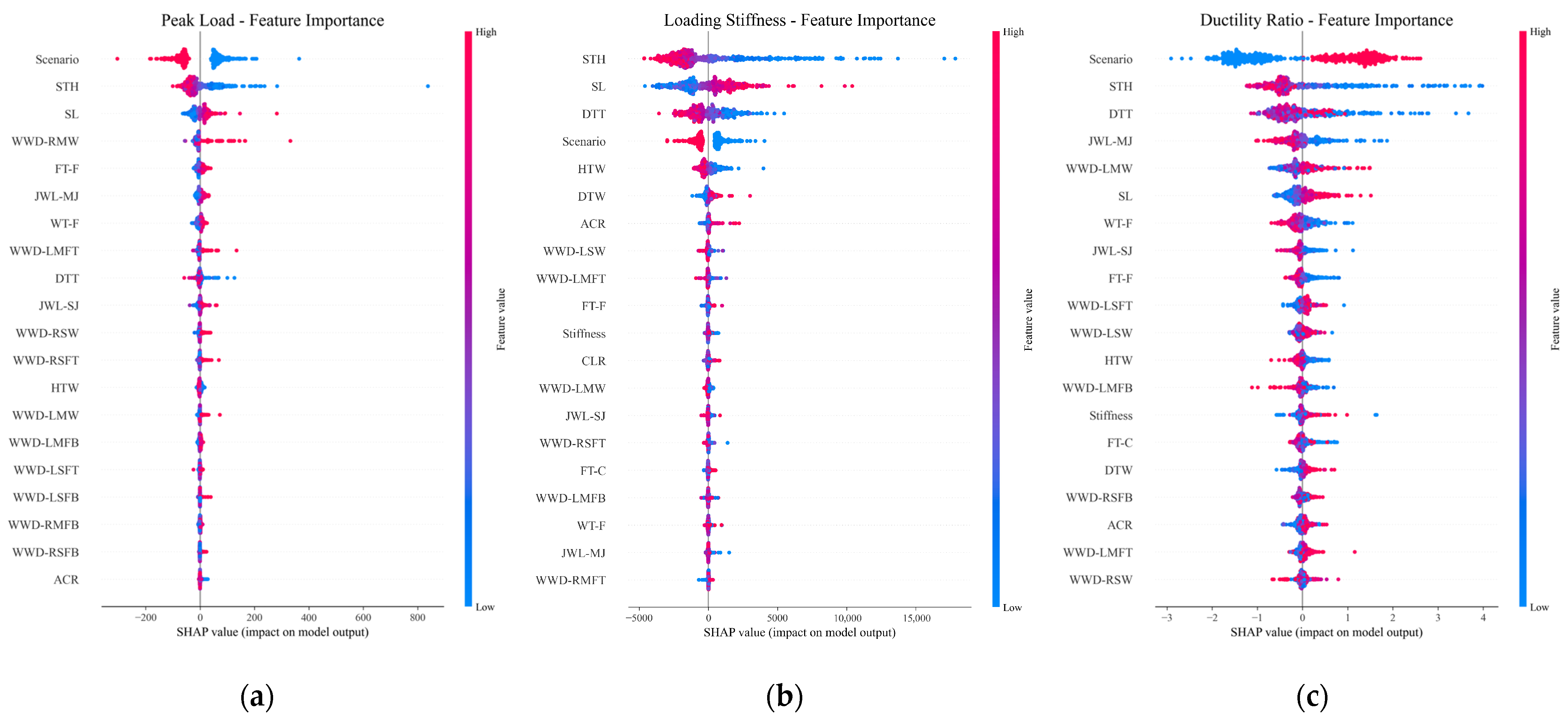
Figure 28 displays a summary plot of the peak load, loading stiffness, and ductility ratio for all samples. The failure scenario is defined as a discrete feature: a value of 1 indicates middle stub failure, while a value of 2 indicates side stub failure. The plot reveals that the middle stub failure scenario contributes positively to the peak load but negatively to the ductility ratio. In contrast, the side stub failure scenario exhibits the opposite contributions. This difference occurs because the development of the flexural action (FA) and catenary action (CA) in the substructure is primarily supported by two span beams under the middle stub failure scenario. Conversely, only a single beam provides the resistance under the side stub failure scenario, functioning as a cantilever beam subjected to a concentrated load. Consequently, the peak load under side stub failure is significantly lower than that under middle stub failure, while the former exhibits better ductility.

Figure 28. SHAP summary plot: (a) Peak load; (b) Loading stiffness; (c) Ductility ratio.

Furthermore, larger beam STH and smaller SL values are disadvantageous for the peak load, initial stiffness, and ductility ratio, as indicated by their negative SHAP values. A larger FT enhances the peak load and loading stiffness but reduces ductility, with WT exhibiting a similar influence. A smaller JWL results in a lower peak load, greater loading stiffness, and improved ductility. For circular steel tube stubs, a larger DTW enhances the loading stiffness and ductility ratio, whereas a larger DTT decreases both.

5.3. Feature Interaction

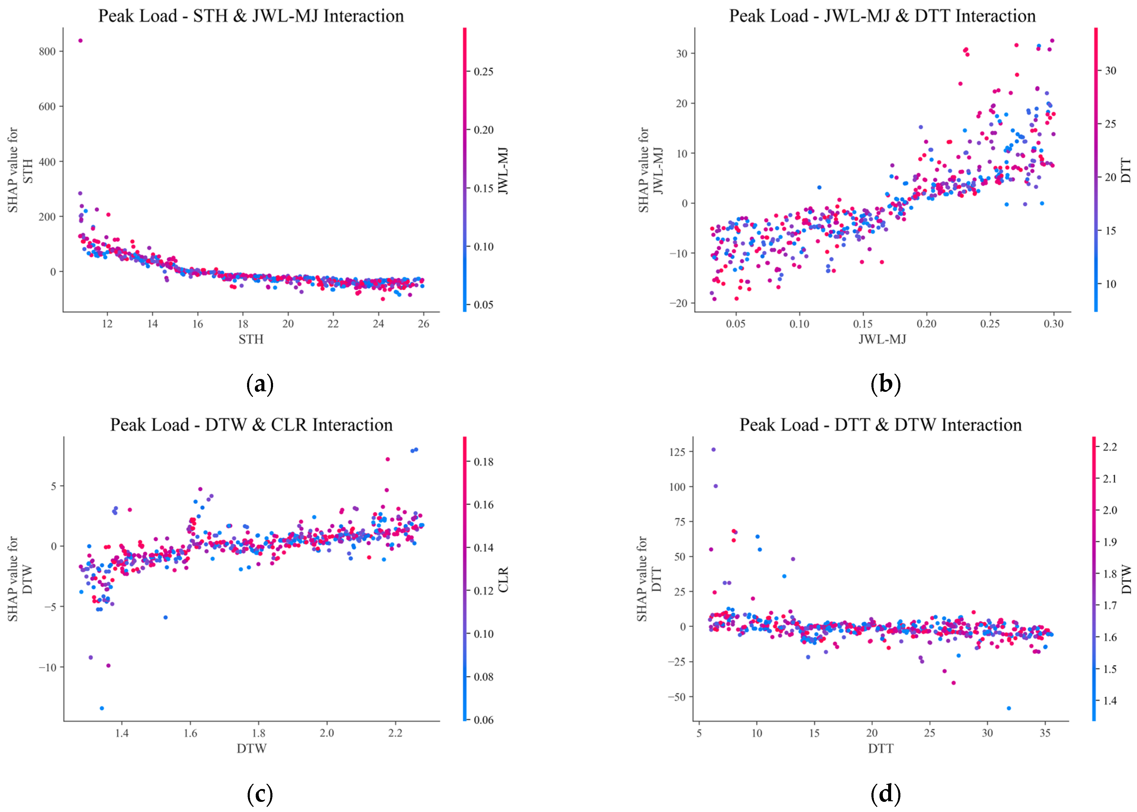
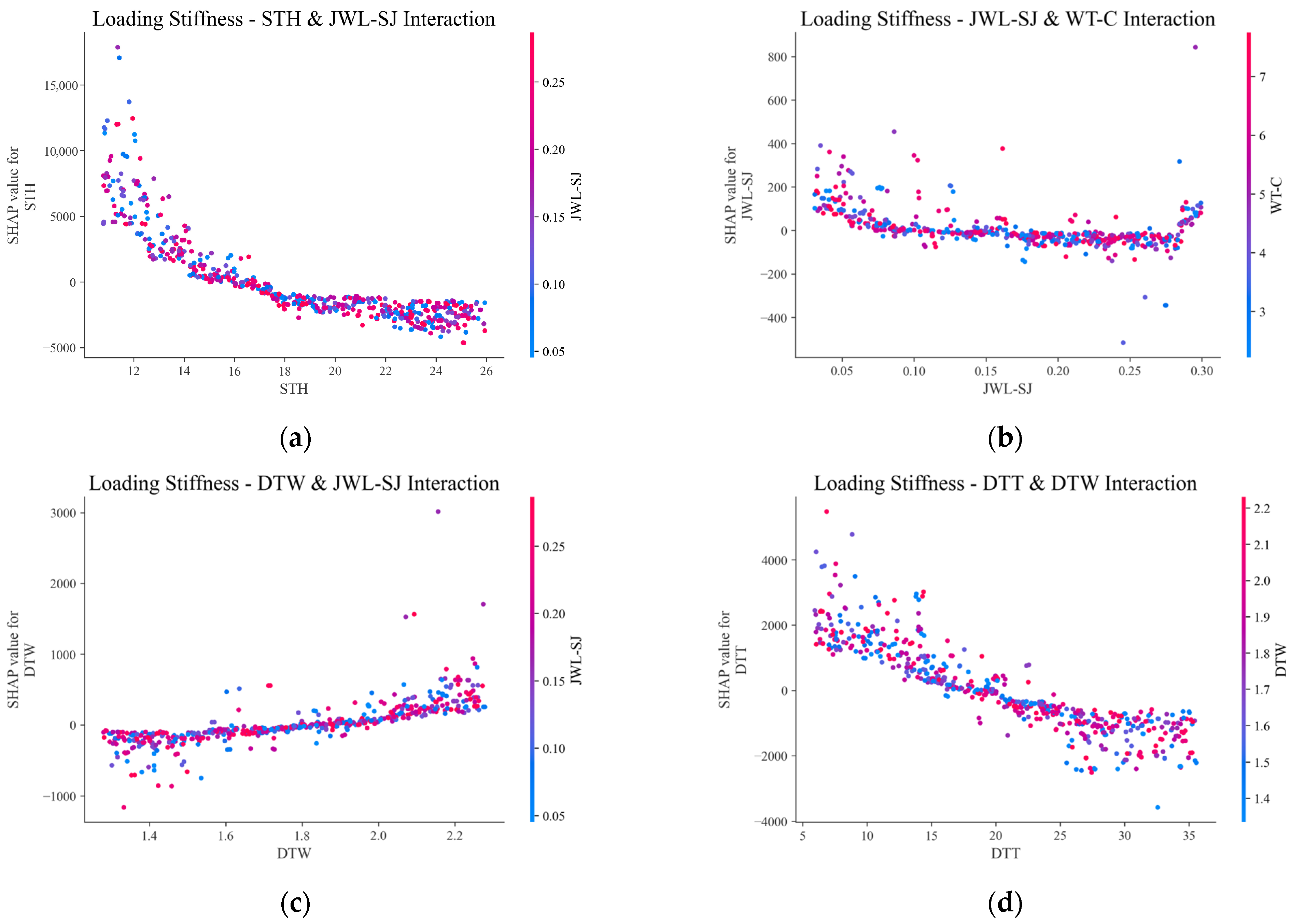
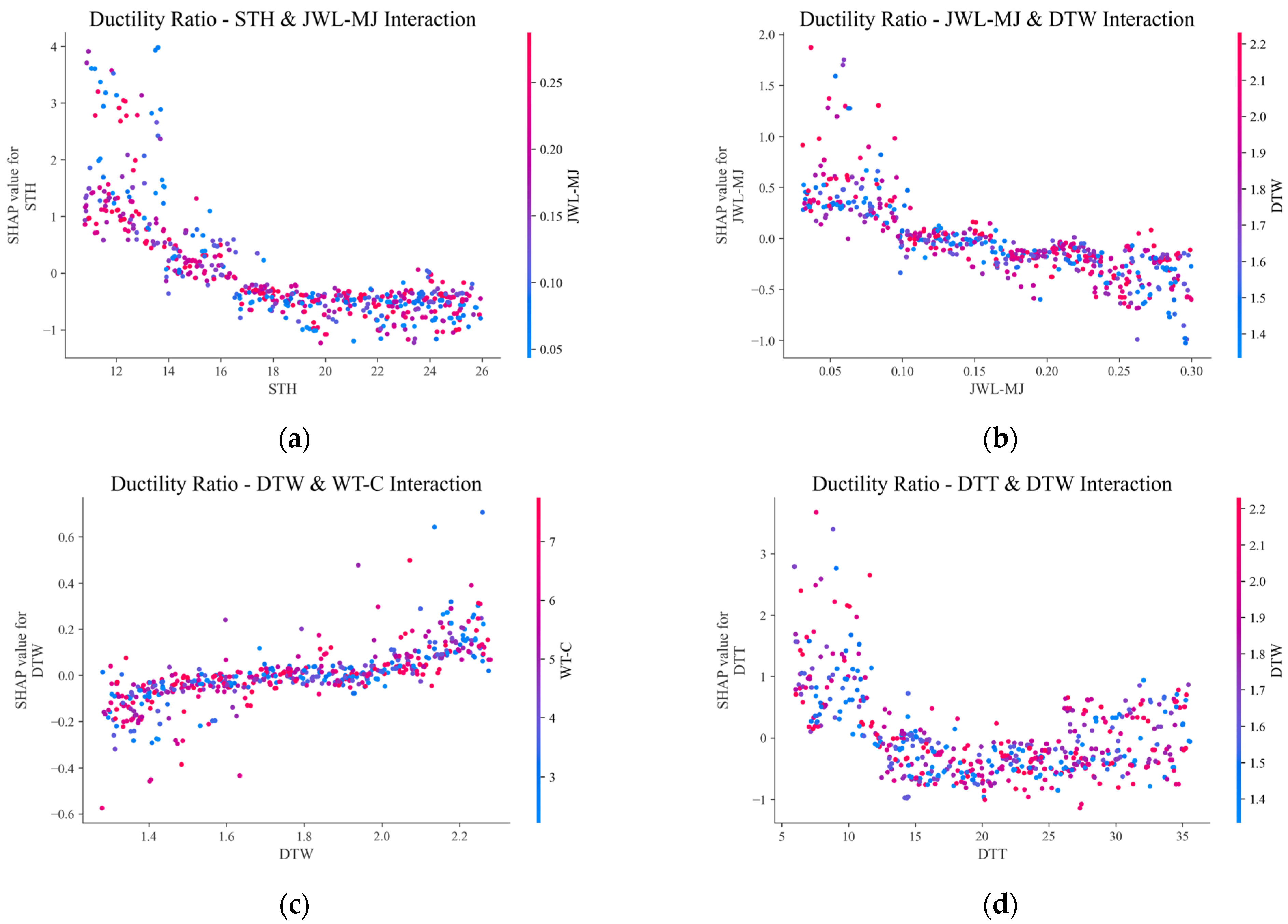
Figure 29, Figure 30 and Figure 31 illustrate the feature interactions among the four primary features (STH, JWL, DTW, and DTT) from a structural design perspective in terms of peak load, loading stiffness, and ductility ratio. The horizontal axis represents the feature value, while the left vertical axis shows the corresponding SHAP value. A positive SHAP value indicates that the current feature value contributes to performance improvement. By examining the regions where negative SHAP values are predominantly distributed for each feature, a structurally reasonable range for these features can be roughly determined when the weld quality at joints is unknown, in order to maximize the robustness of the structure during progressive collapse.

Figure 29. Feature interaction for the peak load: (a) STH; (b) JWL-MJ; (c) DTW; (d) DTT.

Figure 30. Feature interaction for the loading stiffness: (a) STH; (b) JWL-SJ; (c) DTW; (d) DTT.

Figure 31. Feature interaction for the ductility ratio: (a) STH; (b) JWL-MJ; (c) DTW; (d) DTT.

For the peak load, a positive SHAP value generally corresponds to an STH lower than 13, a JWL higher than 0.17, a DTW higher than 1.7, and a DTT lower than 15. For loading stiffness, a positive SHAP value is typically associated with an STH lower than 16, a JWL lower than 0.15, a DTW higher than 1.8, and a DTT lower than 15. For the ductility ratio, a positive SHAP value usually indicates an STH lower than 15, a JWL lower than 0.13, a DTW higher than 1.8, and a DTT lower than 12.

While smaller STH, larger DTW, and smaller DTT enhance the progressive collapse resistance of purely welded steel frames, a balance must be struck with cost-effectiveness. From a cost perspective, values of STH around 15, DTW around 1.8, and DTT around 13 are considered suitable for engineering practice. Furthermore, while maximizing weld quality assurance is paramount, setting the weld joint relative position ratio (JWL) within the range of 0.15 to 0.18 enables the structure to achieve superior performance in resisting progressive collapse.

Finally, due to uncertainties in weld quality, it is impossible to accurately determine the reduction degree of material properties in the weakened zone without material testing. Therefore, this study establishes a mapping relationship between the approximate range of the reduction degree and the ISO 5817 [49] weld quality grades commonly used in engineering practice, as shown in Table 4. This mapping enables engineers to approximately determine the range of the reduction degree based on the weld quality acceptance grade. Consequently, it facilitates an assessment of whether the structural resistance can effectively develop up to the 0.2 rad displacement angle limit specified in the GSA 2016 guideline [4].

Table 4. Mapping between weld quality levels and material weakening degree.

ISO 5817 Quality Levels	Defect Characteristics	Suggested Weakening Degree	Explanation
Level B (Stringent)	Permits only minimal defects. (e.g., undercut depth ≤ 0.5 mm).	100–85%	This level represents high-quality welds. The performance is close to that of the base metal.
Level C (Intermediate)	Allows for defects of certain dimensions. (e.g., undercut depth ≤ 1 mm).	85–60%	This is the common standard for most static structures. A reduction within this range is sufficient to significantly affect structural ductility and collapse resistance.
Level D (Basic)/ Non-Compliant	Permits significant defects or the presence of individual, excessively large defects. (e.g., undercut depth > 1.5 mm).	65–30%	This level corresponds to poor-quality or non-compliant welds. Such welds should be deemed unacceptable on critical load paths for progressive collapse resistance.

6. Conclusions

• An FEM of a steel frame substructure considering weld defects was established and validated by comparing with test results. Subsequently, a parametric modeling program was developed, which employed Latin Hypercube Sampling (LHS) to generate 700 feature combinations from 27 features and to create the corresponding numerical models. Based on the load–displacement angle (P–θ) results from all 700 models, a progressive collapse database was constructed to facilitate machine learning.
• Five machine learning algorithms—DNN, SVR, RF, XGBoost, and LightGBM—were trained on the multi-output database. The SVR algorithm, optimized via Bayesian hyperparameter tuning combined with 5-fold cross-validation, demonstrated the best performance. It achieved an R² of 0.988 and an sMAPE of 5.096% for the full-process load prediction on the test set, indicating high accuracy and strong generalization capability. Compared to theoretical models, the machine learning method can account for the complex effects of weld uncertainty on progressive collapse resistance while enabling efficient prediction, which offers broader applicability.
• SHAP was employed for both single sample and global interpretation to analyze the contribution of each feature to the progressive collapse resistance of substructures. The results revealed that the failure scenario, span-to-height ratio, and weld quality are the three most critical factors, accounting for 22.6%, 22.5%, and 16% of the average importance.
• Engineering practice should prioritize ensuring the weld quality of pure welded steel frames. Considering both cost and progressive collapse resistance performance, this study suggests that a beam span-to-height ratio of approximately 15, stub diameter-to-width of beam ratio of about 1.8, stub diameter-to-thickness ratio of around 13, and weld joint relative position ratio set within 0.15 to 0.18 are suitable for engineering practice.
• Although this study established a mapping between ISO weld quality acceptance grades and the approximate ranges of property weakened degree, it is recommended to directly measure the performance degradation of welding material through tests under identical conditions to ensure accuracy. The proposed machine learning framework is developed for predicting the progressive collapse resistance of purely welded steel frames with box-section beam, with its predictive scope confined to the defined feature domain. However, this framework remains applicable to steel frame structures with bolted or hybrid connections, provided that a representative dataset is available. Additionally, this study does not yet consider the synergistic optimization between structural performance and economic benefits, which could serve as a direction for future research. Finally, while this study focuses on static scenarios based on the alternative load path method, the framework requires further validation and development for dynamic scenarios, such as sudden column loss or blasts and impacts. Such future work should incorporate the effects of material strain rate and structural dynamic response.

References

- Marjanishvili, S.M. Progressive Analysis Procedure for Progressive Collapse. J. Perform. Constr. Facil. 2004, 18, 79–85. [Google Scholar] [CrossRef]
- Shalva, M. Agnew Elizabeth Comparison of Various Procedures for Progressive Collapse Analysis. J. Perform. Constr. Facil. 2006, 20, 365–374. [Google Scholar]
- Sasani, M.; Sagiroglu, S. Progressive Collapse Resistance of Hotel San Diego. J. Struct. Eng. 2008, 134, 478–488. [Google Scholar] [CrossRef]
- General Services Administration (GSA). GSA 2016: Alternate Path Analysis & Design Guidelines for Progressive Collapse Resistance; General Services Administration: Washington, DC, USA, 2016.
- Qian, K.; Liu, Y.; Yang, T.; Li, B. Progressive Collapse Resistance of Posttensioned Concrete Beam-Column Subassemblages with Unbonded Posttensioning Strands. J. Struct. Eng. 2018, 144, 04017182. [Google Scholar] [CrossRef]
- Qian, K.; Li, B. Performance of Precast Concrete Substructures with Dry Connections to Resist Progressive Collapse. J. Perform. Constr. Facil. 2018, 32, 04018005. [Google Scholar] [CrossRef]
- Yang, B.; Tan, K.H. Robustness of Bolted-Angle Connections against Progressive Collapse: Mechanical Modelling of Bolted-Angle Connections under Tension. Eng. Struct. 2013, 57, 153–168. [Google Scholar] [CrossRef]
- Oosterhof, S.A.; Driver, R.G. Behavior of Steel Shear Connections under Column-Removal Demands. J. Struct. Eng. 2015, 141, 04014126. [Google Scholar] [CrossRef]
- Weigand, J.M.; Berman, J.W. Integrity of Bolted Angle Connections Subjected to Simulated Column Removal. J. Struct. Eng. 2016, 142, 04015165. [Google Scholar] [CrossRef]
- Dinu, F.; Marginean, I.; Dubina, D. Experimental Testing and Numerical Modelling of Steel Moment-Frame Connections under Column Loss. Eng. Struct. 2017, 151, 861–878. [Google Scholar] [CrossRef]
- Zhong, W.; Tan, Z.; Tian, L.; Meng, B.; Song, X.; Zheng, Y. Collapse Resistance of Composite Beam-Column Assemblies with Unequal Spans under an Internal Column-Removal Scenario. Eng. Struct. 2020, 206, 110143. [Google Scholar] [CrossRef]
- Zhong, W.; Song, X.; Ma, B. Analysis of Anti-Collapse Performance of Beam–Column Substructure with Welded Flange-Bolted Web Connection in Minor-Axis Direction Under Different Span Ratios. Int. J. Struct. Stab. Dyn. 2018, 19, 1940005. [Google Scholar] [CrossRef]
- Zhang, J.; Jiang, J.; Xu, S.; Wang, Z. An Investigation of the Effect of Semi-Rigid Connections on Sudden Column Removal in Steel Frames. Structures 2018, 13, 166–177. [Google Scholar] [CrossRef]
- Qian, K.; Lan, X.; Li, Z.; Li, Y.; Fu, F. Progressive Collapse Resistance of Two-Storey Seismic Configured Steel Sub-Frames Using Welded Connections. J. Constr. Steel Res. 2020, 170, 106117. [Google Scholar] [CrossRef]
- Qian, K.; Lan, X.; Li, Z.; Fu, F. Behavior of Steel Moment Frames Using Top-and-Seat Angle Connections under Various Column-Removal Scenarios. J. Struct. Eng. 2021, 147, 04021144. [Google Scholar] [CrossRef]
- Yu, P.; Huang, X.; Li, H.; Nie, Y.; He, S. Progressive Collapse Resistance of Unsymmetrical Steel Sub-Structure under a Middle Column-Removal Scenario. J. Build. Eng. 2023, 69, 105994. [Google Scholar] [CrossRef]
- Huang, X.; Elchalakani, M.; Yu, P.; Lin, R.; Nie, Y.; He, S. Progressive Collapse Resistance of Steel Frame with Beam to Column Transfer Structure under a Middle Column-Removal Scenario. Structures 2023, 51, 1–12. [Google Scholar] [CrossRef]
- Yang, B.; Tan, K.H. Behavior of Composite Beam-Column Joints in a Middle-Column-Removal Scenario: Experimental Tests. J. Struct. Eng. 2014, 140, 04013045. [Google Scholar] [CrossRef]
- Yang, B.; Tan, K.H. Experimental Tests of Different Types of Bolted Steel Beam–Column Joints under a Central-Column-Removal Scenario. Eng. Struct. 2013, 54, 112–130. [Google Scholar] [CrossRef]
- Wang, F.; Yang, J.; Pan, Z. Progressive Collapse Behaviour of Steel Framed Substructures with Various Beam-Column Connections. Eng. Fail. Anal. 2020, 109, 104399. [Google Scholar] [CrossRef]
- Huang, X.; Yu, P.; He, S.; Zhang, C. Effects of RWS and Horizontal Restraint on Progressive Collapse of Steel Sub-Structure with Box-Beams. J. Build. Eng. 2025, 104, 112389. [Google Scholar] [CrossRef]
- Shariati, M.; Raeispour, M.; Naghipour, M.; Kamyab, H.; Memarzadeh, A.; Nematzadeh, M.; Toghroli, A. Flexural Behavior Analysis of Double Honeycomb Steel Composite Encased Concrete Beams: An Integrated Experimental and Finite Element Study. Case Stud. Constr. Mat. 2024, 20, e03299. [Google Scholar] [CrossRef]
- Davoodnabi, S.M.; Mirhosseini, S.M.; Shariati, M. Analyzing Shear Strength of Steel-Concrete Composite Beam with Angle Connectors at Elevated Temperature Using Finite Element Method. Steel Compos. Struct. 2021, 40, 853–868. [Google Scholar]
- Yu, P.; Guo, Z.; Yun, W.; Guo, X. Investigation on the New Bolt-Welded Joint of Concrete-Encased CFST under Eccentric Compression. Structures 2025, 72, 108183. [Google Scholar] [CrossRef]
- Guo, Z.; Yu, P.; Huang, X.; Chen, X.; Yao, Y. Numerical Investigation on Dynamic Behaviour of Unbonded Post-Tensioned Precast Concrete Beam Column Sub-Assemblages under Drop Impact Loading. J. Build. Eng. 2025, 113, 113954. [Google Scholar] [CrossRef]
- Kazemi, F.; Shafighfard, T.; Yoo, D.-Y. Data-Driven Modeling of Mechanical Properties of Fiber-Reinforced Concrete: A Critical Review. Arch. Comput. Methods Eng. 2024, 31, 2049–2078. [Google Scholar] [CrossRef]
- Lu, X.-G.; He, Y.; Zheng, W. Design of Advanced Steels by Integrated Computational Materials Engineering. Mater. Genome Eng. Adv. 2024, 2, e36. [Google Scholar] [CrossRef]
- Geng, X.; Wang, F.; Wu, H.-H.; Wang, S.; Wu, G.; Gao, J.; Zhao, H.; Zhang, C.; Mao, X. Data-Driven and Artificial Intelligence Accelerated Steel Material Research and Intelligent Manufacturing Technology. Mater. Genome Eng. Adv. 2023, 1, e10. [Google Scholar] [CrossRef]
- Zhu, Y.F.; Yao, Y.; Huang, Y.; Chen, C.H.; Zhang, H.Y.; Huang, Z. Machine Learning Applications for Assessment of Dynamic Progressive Collapse of Steel Moment Frames. Structures 2022, 36, 927–934. [Google Scholar] [CrossRef]
- Guo, Y.; Yang, B.; Alqawzai, S.; Chen, K.; Kong, D. Machine Learning-Based and Interpretable Models for Predicting the Resistance and Probability of Progressive Collapse of Steel Frame-Composite Floor Structures. Eng. Struct. 2025, 332, 120089. [Google Scholar] [CrossRef]
- Elkady, N.; Augusthus Nelson, L.; Weekes, L.; Makoond, N.; Buitrago, M. Progressive Collapse: Past, Present, Future and Beyond. Structures 2024, 62, 106131. [Google Scholar] [CrossRef]
- Fu, F. Fire Induced Progressive Collapse Potential Assessment of Steel Framed Buildings Using Machine Learning. J. Constr. Steel Res. 2020, 166, 105918. [Google Scholar] [CrossRef]
- Esfandiari, M.; Haghighi, H.; Urgessa, G. Machine Learning-Based Optimum Reinforced Concrete Design for Progressive Collapse. Electron. J. Struct. Eng. 2023, 23, 1–8. [Google Scholar] [CrossRef]
- Esfandiari, M.J.; Urgessa, G.S. Progressive Collapse Design of Reinforced Concrete Frames Using Structural Optimization and Machine Learning. Structures 2020, 28, 1252–1264. [Google Scholar] [CrossRef]
- Hwang, S.-H.; Mangalathu, S.; Shin, J.; Jeon, J.-S. Machine Learning-Based Approaches for Seismic Demand and Collapse of Ductile Reinforced Concrete Building Frames. J. Build. Eng. 2021, 34, 101905. [Google Scholar] [CrossRef]
- Wang, S.; Cheng, X.; Li, Y.; Song, X.; Guo, R.; Zhang, H.; Liang, Z. Rapid Visual Simulation of the Progressive Collapse of Regular Reinforced Concrete Frame Structures Based on Machine Learning and Physics Engine. Eng. Struct. 2023, 286, 116129. [Google Scholar] [CrossRef]
- Gan, Y.; Chen, J.; Li, Y.; Xu, Z. Prediction of Progressive Collapse Resistance of RC Frames Using Deep and Cross Network Model. Structures 2023, 51, 800–813. [Google Scholar] [CrossRef]
- Liu, W.; Zeng, B.; Zhou, Z.; Yao, J.; Lu, Y. Machine Learning-Based Models for Predicting the Progressive Collapse Resistance of Truss String Structures. Eng. Struct. 2024, 307, 117946. [Google Scholar] [CrossRef]
- Olsson, A.; Sandberg, G.; Dahlblom, O. On Latin Hypercube Sampling for Structural Reliability Analysis. Struct. Saf. 2003, 25, 47–68. [Google Scholar] [CrossRef]
- Mostafaei, H.; Behnamfar, F.; Alembagheri, M. Reliability and Sensitivity Analysis of Wedge Stability in the Abutments of an Arch Dam Using Artificial Neural Network. Earthq. Eng. Eng. Vib. 2022, 21, 1019–1033. [Google Scholar] [CrossRef]
- Lundberg, S.M.; Lee, S.-I. A Unified Approach to Interpreting Model Predictions. In Proceedings of the 31st International Conference on Neural Information Processing Systems, Long Beach, CA, USA, 4–9 December 2017; Curran Associates Inc.: Red Hook, NY, USA, 2017; pp. 4768–4777. [Google Scholar]
- GB 50017-2017; Standard for Design of Steel Structures. China Architecture & Building Press: Beijing, China, 2017.
- Eroğlu, M.; Aksoy, M.; Orhan, N. Effect of Coarse Initial Grain Size on Microstructure and Mechanical Properties of Weld Metal and HAZ of a Low Carbon Steel. Mater. Sci. Eng. A 1999, 269, 59–66. [Google Scholar] [CrossRef]
- Jia, Z. Experimental Study on Mechanical Properties of Butt Welded Connection at High Temperature. Master’s Thesis, China University of Mining and Technology, Beijing, China, 2019. (In Chinese). [Google Scholar]
- Kuwamura, H. Classification of Material and Welding in Fracture Consideration of Seismic Steel Frames. Eng. Struct. 2003, 25, 547–563. [Google Scholar] [CrossRef]
- Palanci, M. Fuzzy Rule Based Seismic Risk Assessment of One-Story Precast Industrial Buildings. Earthq. Eng. Eng. Vib. 2019, 18, 631–648. [Google Scholar] [CrossRef]
- Yuan, C.; He, C.; Xu, J.; Liao, L.; Kong, Q. Bayesian Optimization for Selecting Efficient Machine Learning Regressors to Determine Bond-Slip Model of FRP-to-Concrete Interface. Structures 2022, 39, 351–364. [Google Scholar] [CrossRef]
- Ling, H.; Qian, C.; Kang, W.; Liang, C.; Chen, H. Combination of Support Vector Machine and K-Fold Cross Validation to Predict Compressive Strength of Concrete in Marine Environment. Constr. Build. Mater. 2019, 206, 355–363. [Google Scholar] [CrossRef]
- ISO 5817; Welding—Fusion-Welded Joints in Steel, Nickel, Titanium and Their Alloys (Beam Welding Excluded)—Quality Levels for Imperfections. International Organization for Standardization: Geneva, Switzerland, 2023.
Disclaimer/Publisher’s Note: The statements, opinions and data contained in all publications are solely those of the individual author(s) and contributor(s) and not of MDPI and/or the editor(s). MDPI and/or the editor(s) disclaim responsibility for any injury to people or property resulting from any ideas, methods, instructions or products referred to in the content. |
© 2025 by the authors. Licensee MDPI, Basel, Switzerland. This article is an open access article distributed under the terms and conditions of the Creative Commons Attribution (CC BY) license (https://creativecommons.org/licenses/by/4.0/).