A Time Registration Method for Asynchronous Building Electricity Consumption Data Based on the A-PCHIP-iKF Algorithm

Abstract

Building energy consumption data are widely used in various data research and analysis, and data quality is crucial for the accuracy of analysis results. Most existing data quality research focuses on the numerical accuracy of data, while little attention is paid to the temporal accuracy. Time deviations that can be up to thirty minutes are found in the timestamps of the data of a building energy consumption monitoring system. They can result in temporal asynchronism and decreased data accuracy. To correct the time deviations and restore synchronization in data, the A-PCHIP-iKF method is proposed, which integrates time registration and data fusion and utilizes the spatial and temporal correlation to achieve the higher estimation accuracy of correlated time series simultaneously. The results showed that the proposed method has significant advantages over traditional methods in terms of correction accuracy, with 56% RMSE and 60% MAE improvements on the total meter of the building, and can achieve a balance between the correction accuracy, stability, and consistency.

1. Introduction

The operations of buildings account for 30% of global final energy consumption and 26% of global energy-related emissions, and to meet the requirement of the Net Zero Scenario, carbon emissions from building operations need to more than halve by 2030 [1].

Smart buildings are designed to save energy while maintaining acceptable occupants’ comfort by incorporating automation technology and energy and resource management systems within buildings [2]. The extensive deployment of heterogeneous sensors has provided a massive amount of building operational data, which facilitates various energy conservation research, such as energy usage analysis and benchmarking [3], detection of anomalous usage patterns [4], building energy system optimization [5,6], and fault detection and diagnosis (FDD) [7,8].

Good data quality plays an important role in building energy performance analysis [9] and is essential for policy and decision making [10]. A large amount of research effort was invested into ensuring high accuracy of sensor data, including the sensor FDD frameworks of building systems [11,12,13], in situ calibration methods for low-cost environmental monitoring sensors [14,15], sensor calibration based on virtualization techniques [16,17], etc. Despite the great efforts to secure measurement accuracy, building operational data are time series data that consist of an ordered collection of measurement values collected at regular time intervals. Therefore, the accuracy of temporal information is of equal importance as the measurement accuracy. In dynamic data monitoring systems, the timestamp of measurements can be inaccurate due to reasons like inaccurate local clocks, communication delays or network-induced delays, and system processing delays [18,19,20]. Furthermore, in distributed multi-sensor networks, the asynchronization between sensors can be caused by the usage of various types of devices, different transmission protocols, distinct sampling periods, and initial sampling time instants [21,22,23]. Therefore, assuring the temporal accuracy of sensor data and achieving time synchronization is a necessary procedure before multi-source data aggregation and analysis [24].

However, in most existing literature regarding building operational data analysis [25,26], prediction [27,28,29], and quality assessment [30,31], there is a universal absence of reporting checks on the temporal accuracy of the data, and the timestamps of data are assumed implicitly to be synchronous and accurate. Only a few researchers reported performing approximate correction on the timestamp to achieve data synchronization when conducting multi-source data pre-processing. Rusek et al. [32] reported rounding the timestamps of the building users’ subjective comfort opinion data to the nearest 10 min to align with the energy consumption data. Lee et al. [33] reported manually synchronizing the time of different types of measured environmental data using a spreadsheet software. Sözer et al. [34] and Chew et al. [35] both reported matching the time of data collection with different protocols or sampling frequencies, yet without detailed elaboration. Wang et al. [36] mentioned that the sampling between two data acquisition cards was not simultaneous, and the synchronization lag was manually corrected before data analysis. Nevertheless, manually aligning unsynchronized data sequences inevitably disturbs the original correspondence between the measurement value and its timestamp, thereby introducing numerical errors that may exceed the acceptable error limit, especially for dynamic measurements whose value changes drastically with time.

Time registration [37], or time alignment, is the transformation that maps local sensor observation times t to a common time axis t′. This technique has been explored to solve the alignment problem of time series data in fields such as multi-source data fusion [38], target tracking [39], ocean spatial positioning technology [40], head-related virtual acoustics [41], etc. In multi-sensor architectures, a similar process is also referred to as the asynchronous data fusion [42,43,44]. In practice, it is usually preferred to obtain a comprehensive insight from the data of multiple sensors with more accuracy and reliability. Distributed systems such as wireless sensor networks (WSN) [45] are given particular attention due to the limitations of bandwidth and energy. Though with inconsistent taxonomies in the literature [40,42,46,47], common time registration methods include interpolation or curve-fitting methods, least squares methods, the exact maximum likelihood (EML) methods, the Kalman filter and its variants, etc. Chen et al. [39] designed a time registration algorithm based on the spline interpolation applicable to a high-accuracy target tracking system with measurement missing and non-uniform sampling periods. The interpolation methods can adapt to any length of sampling period but are extremely sensitive to measurement errors. Although the curve fitting method can avoid this by setting global smoothness, it has poor adaptability to local conditions. Moreover, both categories lack multivariate data fusion capabilities, limiting their practical applications.

On the contrary, most asynchronous data fusion methods can adapt to centralized or distributed multisensory frameworks, but they are usually limited to specific relationships of sensors’ sampling periods. Zhu et al. [48] proposed sequential asynchronous filter algorithms based on the Kalman filter and particle filter to perform target tracking in asynchronous wireless sensor networks, in which the sampling periods of all sensors were assumed to be the same while the measurements were taken at different time instants. Similar assumptions can be found in [49] by Wang et al., where the starting times of sensors’ measurements are different. For sensors with different sampling periods, certain relationships are also required. Blair et al. [50] originally proposed the least-squares-based time alignment approach for two dissimilar sensors whose sampling rates are in an integer relation. Lin et al. [51] proposed a distributed fusion estimation algorithm for multisensor multi-rate systems with correlated noises, where the state update rate is a positive integer multiple of the measurement sampling rates. Some studies have also examined the situation where time delays exist. Julier et al. [52] proposed the Kalman filter incorporated with the Covariance Union algorithm to address the problem of state estimation for multiple target tracking, where the observation sequences are imprecisely timestamped. However, the delays of the timestamps were assumed to be multiple times the time step of the filter. Similar settings with uniformly spaced time series and random but discrete time delays can be found in [53]. Furthermore, assumptions with different sampling frequencies and initial sampling times were found in [54] by Huang et al., where an adaptive registration algorithm for multiple navigation positioning sensors was proposed based on the real-time motion model estimation and matching using the least squares method and the Kalman filter. A more complicated setup with different and varying sampling periods is adopted in [42], where the spatiotemporal biases of multiple asynchronous sensors were attempted to be simultaneously compensated for data fusion, but the signal transmission delay was assumed to be constant. In summary, asynchronous data fusion, including time registration, is a class of practical engineering problems that are strongly dependent on system architecture, sensor configurations, and problem settings. Therefore, it is crucial to select the appropriate methods based on the problem-specific characteristics.

To the best of the authors, the synchronization and the temporal accuracy of sensory data remain rarely discussed topics in studies related to building energy consumption data. However, most building energy management systems (BEMSs) have a centralized architecture consisting of multi-source heterogeneous sensors, smart meters, and data collectors, where time asynchronism cannot be completely avoided. In addition, most measurement data are measured by meters and sensors, collected by data collectors, and then attached with a unified timestamp and uploaded to data centers [55]. This means that the time delay may accumulate in multiple processes, including data transmission and processing. In this article, based on the analysis of real data from a campus building energy consumption monitoring platform (BECMP), it is proven that both time delays and time asynchronism are found in the timestamps of building energy data. This problem is jointly caused by the characteristics of RS-485 communication and the flawed timestamping mechanism. If not detected, such temporal deviations can greatly affect the data accuracy and introduce uncertainty into the data analysis results.

Most of the existing asynchronous data fusion methods are based on the situation of the same type of sensors [48,49], and have specific requirements for the sampling period of multiple sensors [50,51] or are based on the assumption that the delay is discrete [52,53]. However, in the problem of this paper, the range of time deviation is continuous and random, and the energy consumption monitoring meters in buildings are mostly not equipped with redundant counterparts, which limits the applicability of these methods. Although the spline interpolation method [39] can effectively solve the problem of continuous delay, it may cause oscillation or overshoot for building energy consumption data. Therefore, it is still necessary to study applicable methods for the problem of time deviation correction in BECMPs.

Therefore, improvements to the timestamping mechanism are first proposed, followed by an A-PCHIP-iKF time registration method for the synchronization of the building electricity consumption data with non-negligible time deviations.

The rest of the article is organized as follows. Section 2 gives a detailed analysis of the causes of the time deviation phenomenon of building energy data and its characteristics according to the data collection and transmission process. In Section 3, the A-PCHIP-iKF method is proposed for the correction of data with non-negligible time deviations. In Section 4, the proposed method is compared with traditional methods on simulated data, and the contributions and limitations of the proposed method are discussed. The conclusions of this study are summarized in Section 5.

2. Problem Description

2.1. The Source of Time Deviation

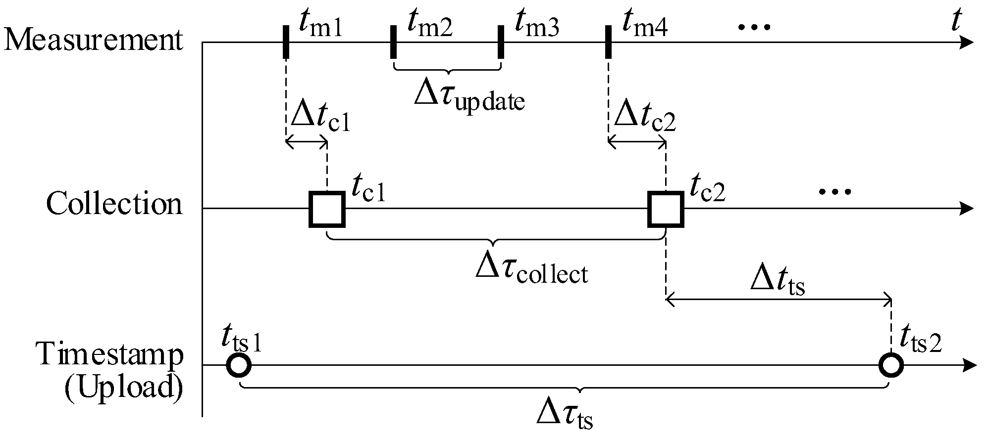
The typical structure of a BECMP is shown in Figure 1. The bottom layer consists of meters and sensors that regularly measure the parameters of interest. In the middle layer, the data collectors perform data collection by acquiring the latest measurements from the registers of meters and sensors with preset frequencies and data buffering by temporarily storing the measurements in the local memory. When the local clock of the data collector reaches a predetermined time for data upload, the data collector packages all the buffered measurements as a data packet with a single timestamp and uploads the packet to the data center. In these processes, the measurement of energy consumption and its timestamping are performed on different devices at different time instants. Therefore, multiple time delays exist, which are summarized in Table 1. The corresponding processes are illustrated in Figure 2.

Figure 1. Typical architecture of a BECMP.

Table 1. Explanation of time delays and time deviations.

Item	Delay Sign	Order of Magnitude	Influence
Measuring delay	Non-negative	ms~s	Negligible
Data collection delay Δtc	Non-negative	ms~s	Negligible
Timestamping delay Δtts	Non-negative	Normally: s~min Abnormally: ~min	Normally: negligible Abnormally: nonnegligible
Clock offset of the data collector Δtclock	Positive or negative	s~min	Can be corrected by clock synchronization.

Figure 2. Data measuring, collection, and timestamping processes.

(1) Measuring delays of sensors

The response of meters may be delayed from the actual change of the target physical quantity due to various factors, and it takes time for the meter to process the measurement and update it on the register. The total delay in such a process is referred to as the measuring delay. In the context of building energy data monitoring, the measuring delay is assumed to be negligible compared to the usual minimum data upload frequency of 15 min to 1 h.

(2) Data collection delays of data collectors

The collection delay Δt_c is defined as the duration from the time the latest measurement is updated by a meter to the measurement is collected by a data collector. It is mainly determined by the relative temporal relationship between the data collections and the register updates, as well as the transmission latency of the communication bus.

For example, as illustrated in Figure 2, a meter updates its measurements with a fixed interval Δτ_update and a data collector performs data collections with a fixed interval Δτ_collect. Two consecutive data collections, c₁ and c₂, correspond to the measurements m₁ and m₄, respectively, and the collection delays Δt_c1 and Δt_c2 can be different due to the non-integer multiple relationship between the two intervals.

The data collection delay is assumed to be negligible in this study.

(3) Timestamping delays

The timestamping delay Δt_ts is the duration from the time a measurement is collected by a data collector to the time the measurement is attached with a timestamp. As mentioned, the timestamp is only attached by a data collector when a data packet is uploaded, rather than immediately after data measuring. Such a mechanism is regulated by the current national technical specification for building energy monitoring [56]. However, for all meters on the same RS-485 bus, the data collections are executed in a polling manner due to the half-duplex communication mechanism, which means the actual collection time t_c for each measurement is unique. Since all measurements share a uniform timestamp, their timestamping delays are non-uniform. Therefore, the timestamping delay of a measurement is mainly determined by its order in the data collection queue before each data upload, which may vary in each cycle.

For example, as shown in Figure 3, a data collector collects the measurements of three parameters, c₁, c₂, and c₃, in a polling manner in a data uploading cycle Δτ_ts, starting with c₃ at time t_c3″ and ending with it at time t_c3′. Before the data uploading time t_ts, the latest measurements of the three parameters are collected at t_c1, t_c2′, and t_c3′. Therefore, their timestamping delay are Δt_ts1, Δt_ts2, and Δt_ts3, respectively.

Figure 3. Detailed data collection process of a data collector.

The inherent asynchronism of data collections of different meters has two aspects of impact. Firstly, in a data upload cycle, although all measurements share a uniform timestamp, their actual times of data measuring are in sequence rather than synchronized. Secondly, the order of meters in the data collection queue before each data upload may vary; therefore, the timestamping delays of a meter in different data upload cycles can be different. This means that for each meter’s sequence of measurements, its actual timestamps may not be uniformly spaced on the timeline. Both impacts are illustrated in Figure 4.

Figure 4. The asynchronism of actual data measuring of different meters.

(4) Abnormal timestamping delays

Normally, the timestamping delay is about seconds to minutes, which is negligible in most cases. However, in practice, a randomly occurring data-collecting failure phenomenon was observed, where the latest value of a parameter cannot be successfully collected. Possible reasons for this phenomenon are electromagnetic interference, poor wiring, and defects in devices. The failure may occur multiple times consecutively, but it can usually recover automatically.

If such a failure happens before data uploading and has lasted for less than a certain number of times, the data collector will upload its last normally collected measurement as a substitute. This is a remedy for uploading a null value, but it also means the timestamping delay of the substitute is much larger than the normal one. For example, in Figure 3, the collection of c₁ failed at t_c1′ before data upload, and its substitute is collected at t_c1, whose timestamping delay is Δt_ts1, which is larger than the normal timestamping delays Δt_ts2 and Δt_ts3.

The existence of abnormal timestamping delay can exacerbate the asynchronism of measurements. Depending on the number of parameters to be collected and the times of data collection failures, abnormal timestamping delays can range from tens of seconds to several minutes. It has a significant negative impact on data accuracy and needs to be addressed with emphasis.

(5) Clock offset of the data collector

The local clock of the data collector may accumulate errors if not calibrated regularly, resulting in seconds to minutes of clock offset. However, it can be directly corrected using the network time protocol (NTP). Therefore, it is feasible to eliminate the clock offset and achieve clock synchronization between all data collectors and the data center servers.

(6) Total time deviation of the timestamp

Total time deviation is the sum of all delays and the clock offset. As mentioned above, the measuring delay and data collection delay are negligible, and the data collector clock can be directly synchronized. Therefore, the total time deviation mainly depends on the timestamping delay, especially the abnormal one.

2.2. The Characteristics of Time Deviations

The time deviation can result in the misalignment between the measured value and its timestamp. If the value of the measured variable changes during the interval, there will be a numerical deviation in the measurement. For energy usage values, time deviations will result in the wrong attribution of energy usage between the adjacent intervals, as illustrated in Figure 5. In the interval from t₁ to t₂, if there are time deviations on both the starting point and the ending point of the interval and the actual times of measuring are t′₁ and t′₂, respectively, then the measured energy usage is W₀ + W₁ while the true value is W₀ + W₂, and the measurement error equals W₁ − W₂.

Figure 5. The effect of time deviation on numerical accuracy.

However, in BECMPs, the energy usage in an interval is calculated by the difference between the two cumulative energy consumption values measured by the electricity meter at the interval endpoints. Therefore, the true energy usage from t₁ to t₂ cannot be acquired due to the lack of true cumulative values at t₁ and t₂. In this study, a campus building is chosen for real data analysis, in which the primary and secondary circuits are fully monitored with sub-metering, and thus the energy usage values of the sub-meters can be summed up to be compared with that of the total meter.

Reasons for the difference between the energy usage values measured by the total meter and that by all the submeters (hereinafter referred to as total-sub difference) include the measuring error of meters, numerical deviations caused by the time deviation, line losses, and unaccounted-for energy consumption of unmeasured secondary circuits.

Figure 6 shows the distribution of the total-sub difference of the same group of meters in a year with different time granularities. Firstly, the relative total-sub difference of hourly, daily, and monthly data are analyzed, including both normal and abnormal data from all meters. For daily and monthly data, the relative total-sub differences are under 5% with the presence of abnormal data, indicating the time deviations’ negligible influences on these scales. The total meter’s values are consistently larger than the summation of the submeters’ values, which points to possible line losses or other measurement-related factors. On the other hand, the relative total-sub difference of hourly data exhibits a much wider and symmetrical distribution, ranging between ±25%. On the basis of the measurement-related factors contributing less than 5% total-sub difference, the large difference of the hourly data points to a more dominating factor, which is the time deviations.

Figure 6. Relative total-sub differences of hourly, daily, and monthly data.

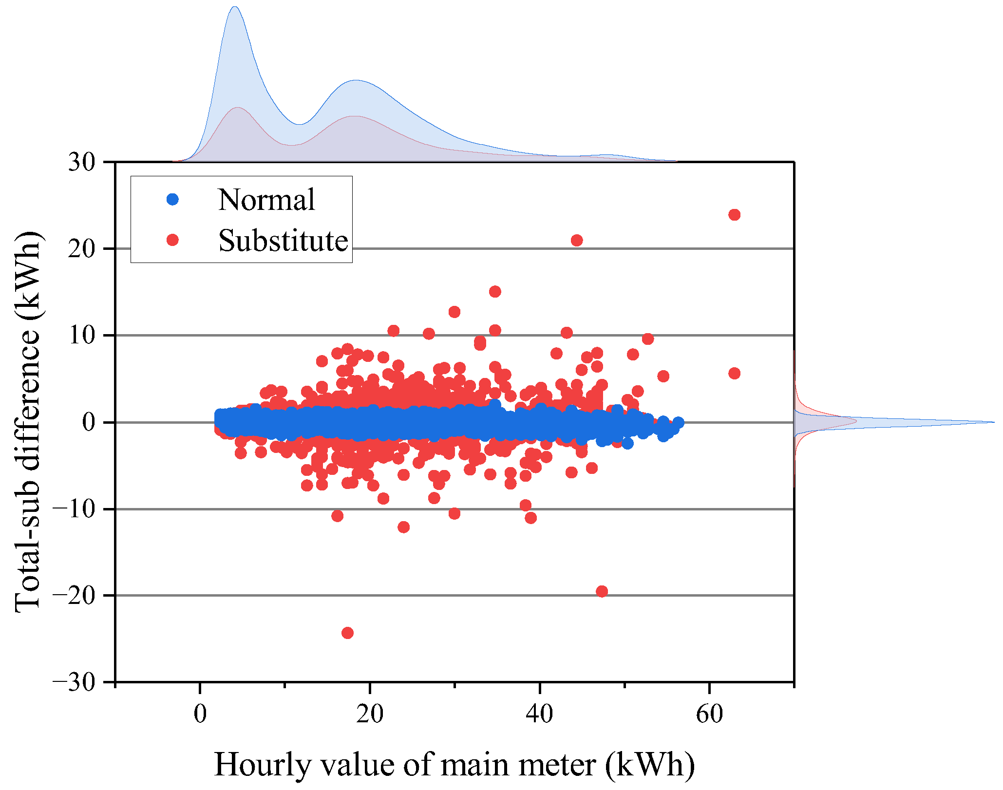
The data collectors used in the platform are designed to attach data collection status codes, which can help with the differentiation of normal and abnormal data. With a zoom-in inspection of the hourly data, the normal values of the submeters are sorted out and summed up to compare with the data of the total meter, which is classified into normal and substitute categories using status codes, as shown in Figure 7.

Figure 7. Hourly total-sub difference classified by the status codes of the total meter.

The total-sub differences of both categories are not strictly equal to zero but are distributed symmetrically around zero. For the normal category, the total-sub difference approximately follows a normal distribution with a mean of 0.13 kWh and a standard deviation of 0.44 kWh, while the abnormal category’s mean is 0.14 kWh and the standard deviation is 2.02 kWh. Evidently, both normal and substitute measurements of the total meter have numerical deviations, while the deviations of the latter are much larger. With a rough estimation by dividing the total-sub differences by the corresponding relative true values, the total meter’s abnormal time deviations can be up to 30 min, while those of the normal ones are mostly within five minutes.

Two other buildings were inspected following the same procedure using the data collection status codes, and substitute data of the buildings’ total meters were also found, although with relatively smaller ranges of numerical deviations. With an expanded inspection of all 7451 electricity meters’ historical data in the platform’s database, about 70% of the meters exhibited substitute data. The highest meter-wise abnormal data proportion during the four years was 59%. Obviously, this issue is not an isolated case.

The time–frequency characteristic of the collection failure is highly random. Figure 8 shows the time series of the hourly energy consumption of a meter, in which the abnormal collected data are marked differently. Based on the analysis of historical data, such phenomena mostly emerge from the very beginning of the platform’s operation, and are mostly contributed to by certain specific meters, indicating the strong correlation with specific equipment defects or low wiring quality.

Figure 8. Example of abnormal data occurrence frequency.

2.3. The Necessity of Correcting Time Deviation

Time deviation can cause reduced data accuracy and time synchronization, leading to the distortion of data patterns and thereby pseudo characteristics, which may result in misleading conclusions and decisions in building-energy-data-related studies. The temporal accuracy of building energy data also plays a vital part in the carbon neutrality goal, where the dynamic carbon emission factors [57] of power grids could be used for the carbon accounting of building end-users. The synchronization of electricity usage data and dynamic carbon emission factors is crucial for the precise calculation of carbon emissions.

In BECMPs, time accuracy is particularly crucial for meters that monitor the energy consumption of an entire building or a larger scale, of which the energy consumption rate is usually high, and even small temporal deviations can result in great numerical deviations. Such meters are often used as analysis objects or data sources in research and applications, making the correction of time deviation in such scenarios extremely important.

3. Methodology

In this study, the correction of abnormal time deviations is mainly studied due to their great influence on data accuracy. An additional assumption is made that the accurate measuring times of the substitute data are known. Although such information is currently unavailable due to the restriction of the regulations, the modification of the timestamping mechanism of the data collectors is feasible and necessary. On the other hand, the intention of uploading substitutes is to remedy uploading null values and preserve the original information as much as possible. Without timestamps representing the actual times of measuring, the substitute data cannot be accurately positioned on the timeline, thereby losing their effectiveness in evaluating the degree of the temporal deviation and in providing a basis for data correction. Under such a condition, the problem is essentially equivalent to performing data imputation in the absence of the substitute data.

To correct the time deviations, a two-step framework is proposed, consisting of a time registration procedure utilizing the temporal correlation of each meter’s time series data, and a data fusion procedure where the spatial correlation of the building’s total meter and sub-meters is comprehensively utilized.

3.1. Time Registration

The energy consumption behavior of buildings usually has short-term and long-term temporal regularity that can be utilized for forecasting and regression. Long-term regularity is mainly manifested in the periodic and seasonal patterns of energy consumption data on a month or yearly scale, which are driven by external climate conditions and inherent characteristics of the building. However, due to the randomness of the collection failure phenomenon described in Section 2.2, it is difficult to obtain sufficiently long and error-free historical time series of the target meter to perform statistical and machine learning methods like ARIMA [58] and artificial neural networks that require enough data for modeling or training. Moreover, the abnormally collected data points of the time series are not equally spaced on the time axes, which do not meet the requirements of common methods for dealing with time series, such as LSTM [59].

Short-term regularity manifests as the high-frequency and periodic fluctuations of the energy consumption curve within a 24-h period, whose driving factors are mostly human activities. Considering the length of time, deviations are mostly less than one hour, the utilization of short-term patterns can be further shortened to the local trend of the energy consumption curve, which can be only several hours around the temporally deviated data point. As simple yet efficient time registration techniques, interpolation methods do not require equal time intervals or model training using historical data and are suitable for utilizing the local characteristics of curves. Most importantly, interpolation methods can effectively cope with the continuous value range of the time deviation problem in this study.

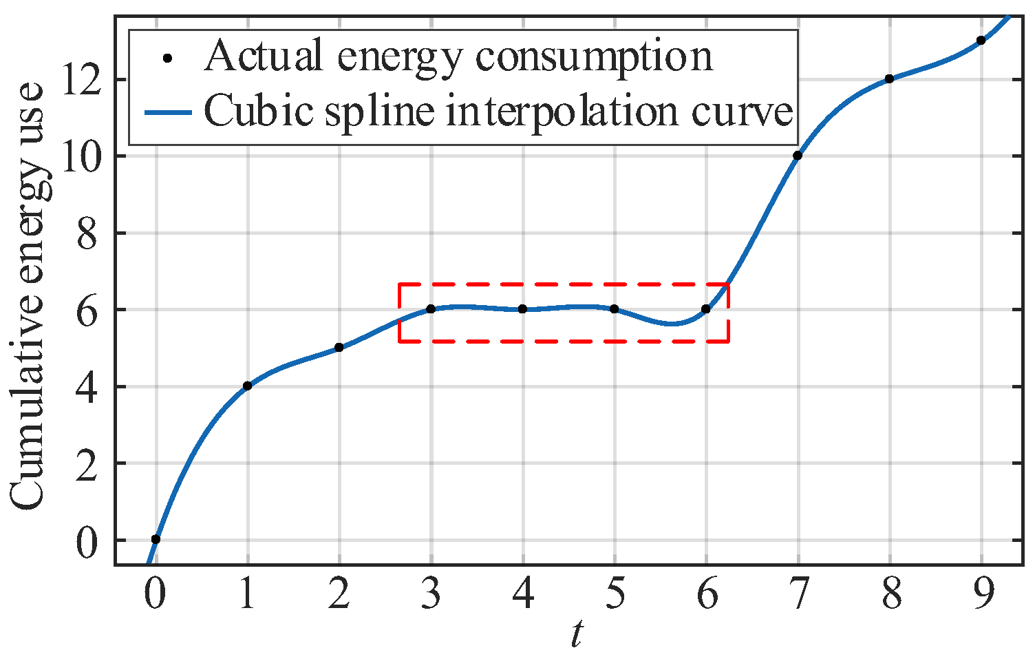
Among interpolation algorithms, the commonly used B-spline and cubic spline methods emphasize the smoothness of the interpolation curve, and the continuity of the higher derivative of the spline function is usually required. This makes them lack the ability to preserve monotonicity and are unsuitable for tracking the cumulative building energy consumption curves, as the latter may remain unchanged during idle hours, while the spline interpolation curve may exhibit fluctuations that do not conform to physical laws, as shown in Figure 9.

Figure 9. Fluctuated curve of cubic spline interpolation during idle hours.

The piecewise cubic Hermite interpolating polynomial (PCHIP) [60] is a category of interpolants including the spline interpolants and others, but with various settings of derivatives. Currently, the PCHIP function in scientific computing tools like MATLAB 2025a and SciPy 1.16.0 adopts the derivatives setting originally proposed by Fritsch et al. [61] for its shape-preserving ability. Therefore, it is employed for time registration in this study for its monotonicity-preserving ability for cumulative building energy consumption values. However, in Fritsch’s original design, the weight coefficients used to calculate the derivative values were a fixed linear combination of the lengths of adjacent intervals. This made it lack the ability to adapt to specific data characteristics. Therefore, an adaptive PCHIP method is proposed in this study, which optimizes the interpolation parameters through a data-driven approach and is particularly suitable for the time registration of time series of cumulative building energy data.

3.1.1. Adaptive PCHIP

Consider the time series (t_i, y_i), i = 1, 2, …, N, where the timestamps of normal data points are accurate and uniformly spaced from each other, while the timestamps of the sparsely distributed substitute data are deviated from the standard time instants. The base function of PCHIP for any data point at t ∈ [t_i, t_{i + 1}] is:

$$y\left(t\right)=h_{00}\left(s\right)\cdot y_i+h_{10}\left(s\right)\cdot h_i\cdot d_i+h_{01}\left(s\right)\cdot y_{i+1}+h_{11}\left(s\right)\cdot h_i\cdot d_{i+1}$$

(1)

where the normalized local variable s = (t − t_i)/h_i, the length of the interval h_i = t_{i + 1} − t_i, and the coefficients of the base function are h₀₀(s) = (1 + 2s)(1 − s)², h₁₀(s) = s(1 − s)², h₀₁(s) = s²(3 − 2s), h₁₁(s) = s²(s − 1).

At any known internal data point at t_i (2 ≤ i ≤ N−1), the derivative d_i is calculated by:

$$d_i=\left\{\begin{array}{cc}0& \mathrm{if} {\delta }_{i-1}\cdot {\delta }_i\le 0\\ {\displaystyle \frac{w_1+w_2}{w_1/{\delta }_{i-1}+w_2/{\delta }_i}}& \mathrm{otherwise}\end{array}\right.$$

(2)

where δ_i is the slope of [t_i, t_{i + 1}] calculated by:

$${\delta }_i={\displaystyle \frac{y_{i+1}-y_i}{h_i}}$$

(3)

w₁ and w₂ are weights determined by the lengths of the two adjacent intervals:

$$w_1={\alpha }_1{h}_i+{\alpha }_2{h}_{i-1}$$

(4)

$$w_2={\alpha }_2{h}_i+{\alpha }_1{h}_{i-1}$$

(5)

where α₁ and α₂ are coefficients to be optimized according to actual time series data.

For any interpolation point, a total of four known data points is required to calculate the function value, with two points on each side. Due to the sparsity of the temporally deviated data points, it is always possible to find consecutive normal data points as the beginning and end of the entire time series to be interpolated. Therefore, the special treatment of the derivative values at the sequence endpoints can be omitted.

3.1.2. Parameter Optimization

In the adaptive PCHIP algorithm, the optimal weight coefficients α₁ and α₂ need to be found such that the mean square error (MSE) of the interpolation result on the validation set is minimized. The Leave-One-Out Cross-Validation (LOOCV) strategy is employed to construct the loss function for parameter optimization. The method is capable of providing a near-unbiased global evaluation of the model performance due to the employment of all internal data points of the entire time series. The overall process of the method is, for a dataset containing N samples, N rounds of training and validation are conducted, and within each round, N-1 samples are used as the training set and the remaining one sample is used as the validation set. Finally, the average error of all N validations is calculated as the evaluation of the model’s performance.

The loss function is defined as:

$$L({\alpha }_1,{\alpha }_2)={\displaystyle \frac{1}{N}}\sum _{i=1}^N{\left(y_i-{\widehat{y}}_i^{(-i)}({\alpha }_1,{\alpha }_2)\right)}^2$$

(6)

where y_i is the truth value of the ith data point, ${\widehat{y}}_i^{(-i)}({\alpha }_1,{\alpha }_2)$ is the prediction value using coefficients α₁ and α₂ with the ith data point excluded.

Moreover, to ensure that the weight coefficients do not become too small and thus lead to unstable values, or too large and cause overfitting, the coefficients are subjected to the constraints:

$$0.1\le {\alpha }_1,{\alpha }_2\le 10.0$$

(7)

The minimization of the loss function described in (6) is solved using the L-BFGS-B algorithm, a limited-memory quasi-Newton method designed for large-scale optimization problems with bound constraints [62]. This algorithm effectively exhibits robust performance for non-linear and non-convex objective functions and can incorporate constraints on the coefficients.

The convergence conditions include:

• The norm of the gradient is sufficiently small:

$$‖\nabla L^{\left(k\right)}‖<{\epsilon }_{\mathrm{grad}}$$

(8)

• The change in parameters is sufficiently small:

$$\left|{\alpha }^{(k+1)}-{\alpha }^{\left(k\right)}\right|<{\epsilon }_{\mathrm{param}}$$

(9)

• The change in the loss function is sufficiently small:

$$\left|L^{(k+1)}-L^{\left(k\right)}\right|<{\epsilon }_{\mathrm{loss}}$$

(10)

• The maximum number of iterations is reached.

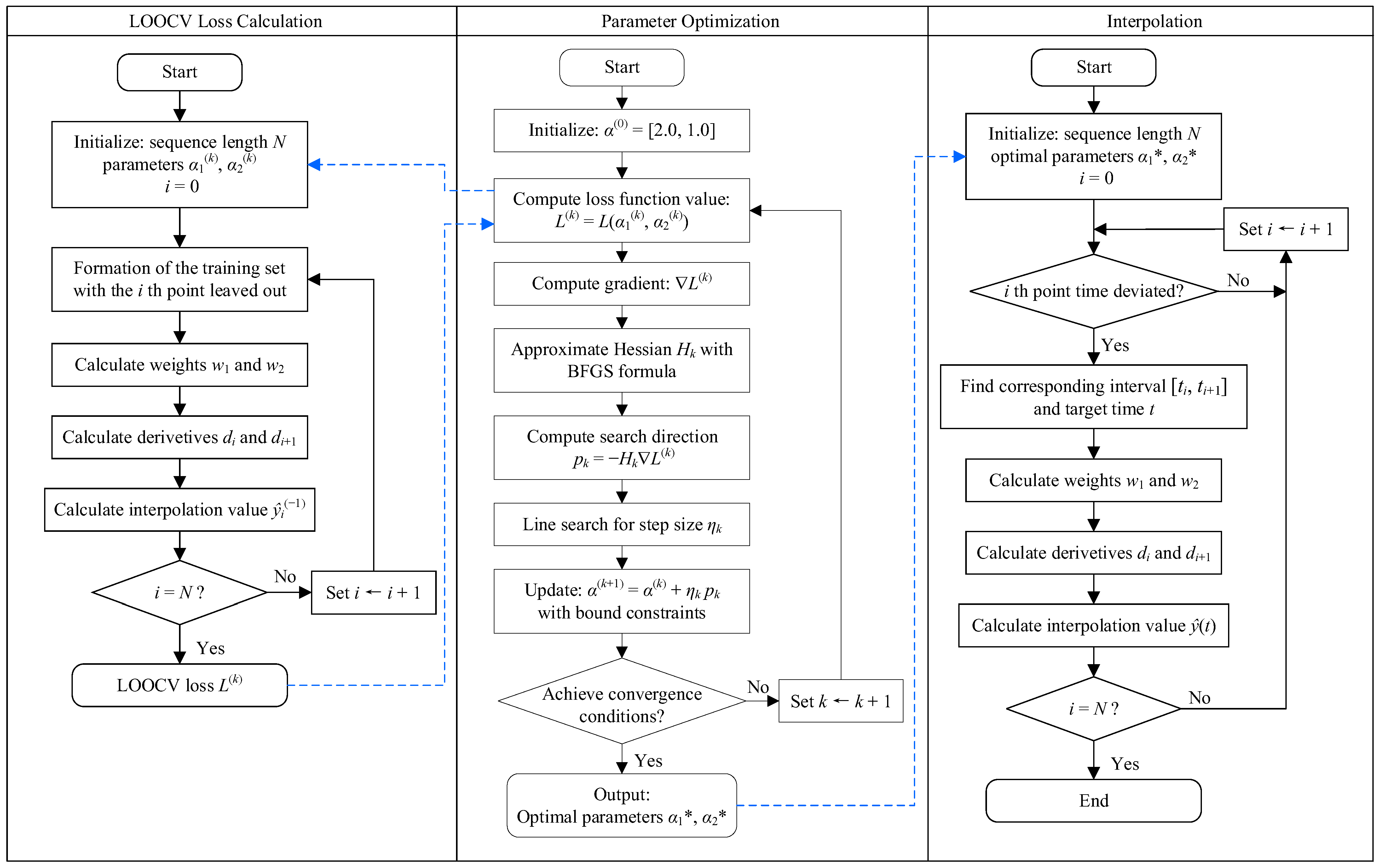
The flowchart illustrating the workflow of the A-PCHIP method, including the calculation of the LOOCV loss function, parameter optimization and interpolation, is shown in Figure 10.

Figure 10. Flowchart of the A-PCHIP method (Blue dashed lines represent the logical relationship between methods).

3.2. Iterative Data Fusion

Estimates obtained through time registration may contain estimation errors, and the estimates of correlated meters may conflict with each other and break the law of conservation of energy. Therefore, to ensure physically meaningful results of correlated meters and achieve higher estimation accuracy, it is necessary to correct the preliminary estimation errors utilizing the spatial correlation of meters as the limiting boundary condition.

The Kalman filter (KF), as a commonly used data fuser, is an efficient autoregressive filtering model consisting of a set of equations that can estimate the optimal state of a dynamic process in terms of minimizing the mean squared error (MMSE) [63], even when the precise nature of the modeled system is unknown [64]. By recursively applying the “prediction” and “correction” process, it only needs to retain the current system state data [65]. Therefore, it is suitable for the correction of time deviations in this study.

However, in most BECMPs, redundant sensors are unavailable, which means the common condition of multiple sensors monitoring the same target cannot be satisfied. Therefore, the proposed data fusion technique adopts the implementation of an iterative Kalman filter (iKF) consists of two iteratively executed steps: the generation of the virtual meter and the measurement fusion. Firstly, select the set of a total meter and submeters {m₀, m₁, m₂, … m_M} whose normally collected data satisfy the law of conservation of energy. Secondly, repeatedly execute the generation of a virtual meter and the data fusion, starting from m₀ and ending with m_M. Meanwhile, when each data fusion process is completed, the fused time series is then used for the generation of the next virtual meter, replacing its unfused one. Finally, when the fused time series of the last submeter is obtained, all fused series of submeters are used for the last round of virtual meter generation and data fusion for the total meter.

3.2.1. The Generation of Virtual Meters

The virtual meter of each meter is generated using the time series of all the other meters, which includes the time-registered series E_m,R, or the fused series E_m,F, if the latter are available.

The virtual measurement of the total meter (m = 0) at t can be calculated by:

$$E_0^{\prime }(t)=\sum _{m=1}^M{E}_{m,\mathrm{R}/\mathrm{F}}\left(t\right)$$

(11)

where E_{m, R/F}(t) is the time-registered or fused measurement of submeter m (m = 1, 2, …) at t, and M is the total number of submeters, M ≥ 2. Whenever the fused time series of a meter is available, it is substituted into (11), replacing the unfused one. The measurement of a virtual submeter at time t can be calculated by:

$$E_i^{\prime }(t)=E_{0,\mathrm{F}}(t)-\sum _{m=1}^M{E}_{m,\mathrm{R}/\mathrm{F}}\left(t\right),\hspace{0.33em}\hspace{0.33em}m\ne i$$

(12)

where E_0,F(t) is the fused measurement of the total meter at t.

The measurement values used in Equations (11) and (12) can either be time-segmented energy usage values, like the hourly values, or they can be cumulative energy consumption values if the time series of all the meters are aligned to a relative zero point so that the cumulative energy consumption values can be added up directly. The cumulative values are chosen in this study.

3.2.2. The Measurement Fusion

The second step is the data fusion of the time series of each meter and its virtual meter using the Kalman filter, where the time series E_j(t) and E′_j(t) are fused via a measurement fusion model based on the KF [66]. The temporal evolution of cumulative energy consumption can be approximately modeled by the discrete-time linear equation:

$$x_t=A{x}_{t-1}+w_{t-1}$$

(13)

$$z_t=H{x}_t+v_t$$

(14)

where t is the uniformly spaced time index, x_t is the state vector at time t, z_t is the observation vector, w_t-1 and v_t are the uncorrelated zero-mean process noise and measurement noise vector with covariances Q and R_, respectively, and A and H are the state transition and observation matrices.

The system dynamics within each time interval are assumed to be governed by the constant acceleration (CA) kinematic model. The parameters to be estimated in the model are given by the state vector:

$$x_t=\left(\begin{array}{c}x\\ \dot{x}\\ \ddot{x}\end{array}\right)$$

(15)

where x, $\dot{x}$, and $\ddot{x}$ represent the position, velocity, and acceleration components of the system state, respectively. The state transition matrix is:

$$A=\left[\begin{array}{ccc}1& \Delta t& \Delta t^2/2\\ 0& 1& \Delta t\\ 0& 0& 1\end{array}\right]$$

(16)

The position component, i.e., cumulative energy consumption, is an explicit state, while the velocity and acceleration components, i.e., the time-segmented energy usage and its changing rate over time, are hidden states. The observation vector z_t consists of the time series values of the current meter and its virtual meter:

$$z_t=\left[\begin{array}{c}{E}_j\left(t\right)\\ E_j^{\prime }\left(t\right)\end{array}\right]$$

(17)

and the observation matrix is:

$$H=\left[\begin{array}{c}\begin{array}{ccc}1& 0& 0\end{array}\\ \begin{array}{ccc}1& 0& 0\end{array}\end{array}\right]$$

(18)

The state and covariance time propagation equations of the measurement fusion model are:

$${\tilde{x}}_{t+1}^f=A{\widehat{x}}_t^f$$

(19)

$${\tilde{P}}_{t+1}^f=A{\widehat{P}}_t^f{A}^T+Q$$

(20)

where ${\tilde{x}}_{t+1}^f$ is the a priori estimate of the fused state vector at t + 1, ${\widehat{x}}_t^f$ is the posterior estimate of the fused state vector at t, ${\tilde{P}}_{t+1}^f$ is the covariance matrix of the prior estimation error, and ${\widehat{P}}_t^f$ is the covariance of the posterior estimation error. When the noise sequences {w_t} and {v_t} are Gaussian, uncorrelated, and white, the KF is the minimum variance filter and minimizes the trace of the estimation error covariance at each time step.

The state and covariance update equations are:

$$K_{t+1}^f={\tilde{P}}_{t+1}^f{H}^T{\left[H{\tilde{P}}_{t+1}^f{H}^T+R\right]}^{-1}$$

(21)

$${\widehat{x}}_{t+1}^f={\tilde{x}}_{t+1}^f+K_{t+1}^f\left[Z_{t+1}-H{\tilde{x}}_{t+1}^f\right]$$

(22)

$${\widehat{P}}_{t+1}^f=\left[I-K_{t+1}^{f}H\right]{\tilde{P}}_{t+1}^f$$

(23)

where $K_{t+1}^f$ is the Kalman gain, and I is a 3 × 3 identity matrix.

The measurement noise covariance is:

$$R=\left[\begin{array}{cc}{R}_1& 0\\ 0& R_2\end{array}\right]$$

(24)

where R₁ and R₂ are determined by the reconstruction error of the LOOCV process of the adaptive PCHIP using the optimized coefficients. R₁ is the reconstruction MSE of the current meter m:

$$R_{m,1}=L_m({\alpha }_1^{\ast },{\alpha }_2^{\ast })$$

(25)

and R₂ is the sum of the reconstruction MSE of all the other meters:

$$R_{m,2}=\sum _{j=0}^M{L}_j({\alpha }_1^{\ast },{\alpha }_2^{\ast }),\hspace{0.33em}\hspace{0.33em}\hspace{0.33em}j\ne m$$

(26)

The procedure of iKF algorithm is outlined in Algorithm 1.

Algorithm 1: Iterative Kalman filter data fusion

Input: Time registered sequences Em,R, LOOCV losses Lm, m = 0, 1, … , M

Output: Fused sequences Em,F, m = 0, 1, … , M

1: for m ∈ {0, 1, … , M} do

2:      R1 = Lm

3:      R2 = SUM(Lm) – R1

4:      if m = 0 then

5:                 Calculate virtual meter E′0 by Equation (11)

6:       else

7:                 Calculate virtual meter E’m by Equation (12), use fused data if exists

8:       end

9:       /*       Kalman filter initialization    */

10:     Z = [Em, E’m], X_fused = [], P_fused = []

11:     Initialize empirically X_posterior, P_posterior, Q

12:     Add X_posterior to X_fused, add P_posterior to P_fused

13:     Set A, H, R by Equations (16), (18) and (24)

14:     /*       Kalman filter measurement fusion           */

15:     for i ∈ {0, 1, … , N} do

16:               State and covariance propagation by Equations (19) and (20)

17:               Calculate Kalman gain by Equation (21)

18:               State and covariance update by Equations (22) and (23)

19:               Add X_posterior to X_fused, add P_posterior to P_fused

20:     end

21:      /*       Fusion result of current meter        */

22:      Em,F ← X_fused[:, 0, 0]

23:      return Em,F

24: end

25:      /*       Final fusion for the total meter      */

26: Calculate virtual meter E′0 by Equation (11) with all fused sequences Em,F

27: Kalman filter initialization and measurement fusion for Z = [E0, E′0]

28: return E0,F

The flowchart of the proposed iterative data fusion method is illustrated in Figure 11 with an example of five meters.

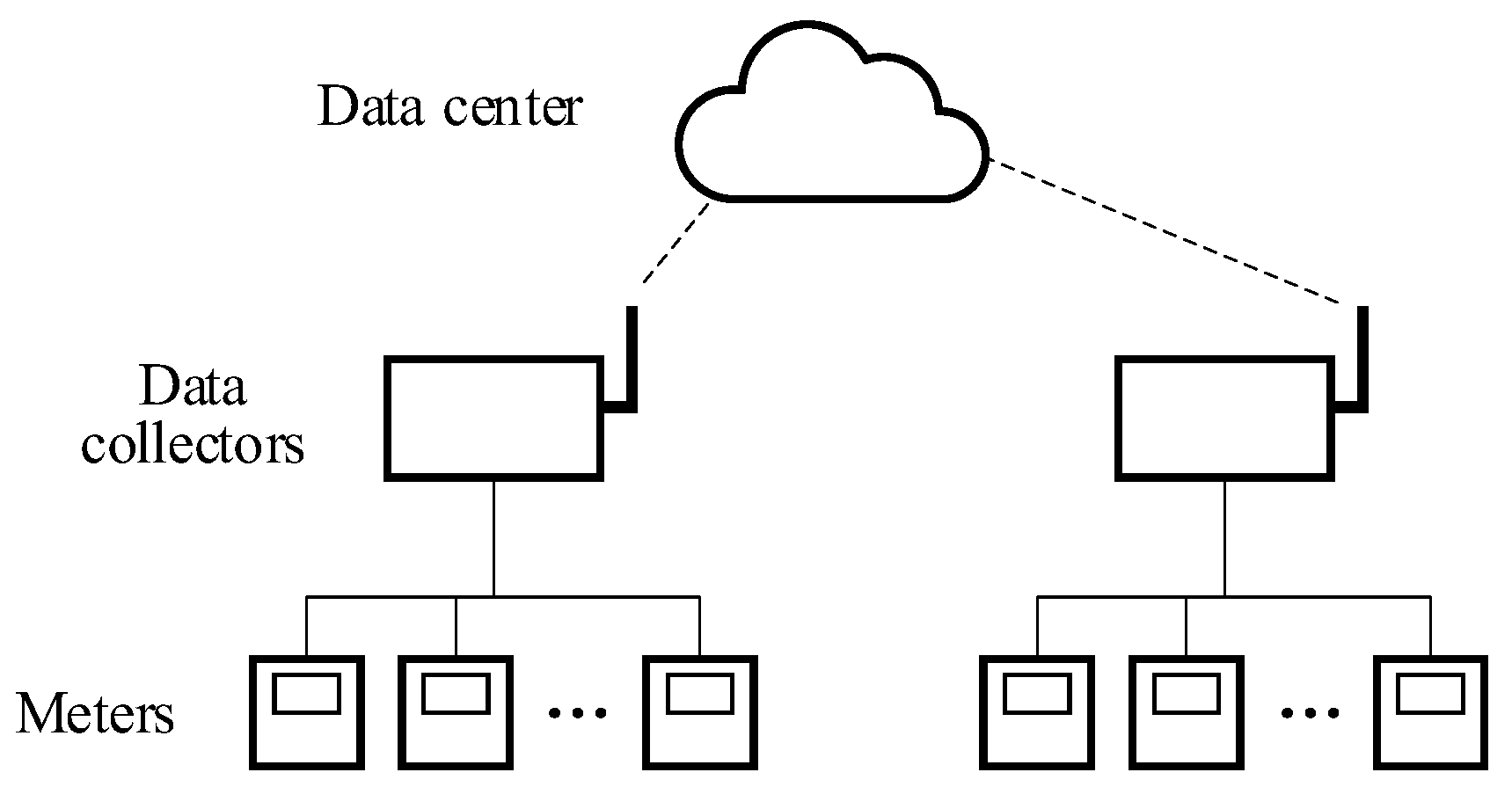
Figure 11. The flowchart of the proposed iterative data fusion method.

4. Results and Discussion

4.1. Simulation Setup

4.1.1. Data Source

The test data are extracted from a campus dormitory building electricity management platform that monitors the energy consumption of 36 dormitory buildings and has been continuously operating since 2016. The data sampling period is 1 h, and the main data types include electricity consumption of dormitory rooms’ lights and plugs, as well as electricity consumption of equipment in public areas such as lighting, water heaters, and washing machines. A typical architectural diagram of the dormitory building circuit system is shown in Figure 12. The building’s total meter has ten submeters downstream, where submeter 1 has six subsequent submeters monitoring the electricity usage of each floor, and each floor meter has twenty-three subsequent submeters monitoring each room.

Figure 12. The typical architectural diagram of the dormitory building circuit system.

4.1.2. Formation of Ground Truth Dataset

Two datasets are formed with different numbers of submeters to validate the correction performance and scalability of the proposed method. Dataset #1 consists of the time series of eight submeters under the building total meter, while two submeters are excluded due to zero electricity usage, as summarized in Table 2. Dataset #2 consists of the time series of twenty-three room meters on the first floor, while three meters are excluded due to the same reason. The basic information of the room meters is summarized in Table 3.

Table 2. Basic information of submeters in Dataset #1.

Meter No.	Circuit Name	Avg. Hourly Electricity Usage (kWh)
Submeter 1	1st to 6th floors lights and plugs	2.58
Submeter 2	2nd floor water heater	1.46
Submeter 3	Auxiliary system	1.62
Submeter 4	4th floor water heater	1.54
Submeter 5	Washing machines room	0.05
Submeter 6	Emergency lighting	0.07
Submeter 7	Public restroom lighting	0.16
Submeter 8	Backup (Unknown purpose)	0.13
(Excluded)	Backup	0.00
(Excluded)	Backup	0.00

Table 3. Basic information of room meters in Dataset #2.

Room No.	Avg. Hourly Electricity Usage (kWh)	Room No.	Avg. Hourly Electricity Usage (kWh)
101	0.024	113	0.008
102	0.024	114	0.041
103	0.007	115	0.008
104	0.012	116	0.006
105	0.013	117	0.011
106	0.045	118	0.022
107 (Excluded)	0.000	119	0.045
108	0.044	120	0.020
109	0.032	121	0.026
110	0.034	122 (Excluded)	0.000
111	0.016	123 (Excluded)	0.000
112	0.021

The chosen time window is from 23:00 on 28 February 2018 to 0:00 on 12 April 2018, to avoid any missing or abnormally collected data points from any of the selected meters. Therefore, each meter’s time series consists of 1010 consecutive normally collected hourly cumulative energy consumption data points, making the two datasets contain a total of 28,280 data points. The start and end times of all sequences were aligned.

All selected meters exhibit different characteristics such as average hourly energy usage level, fluctuation range, and number of peaks in a day.

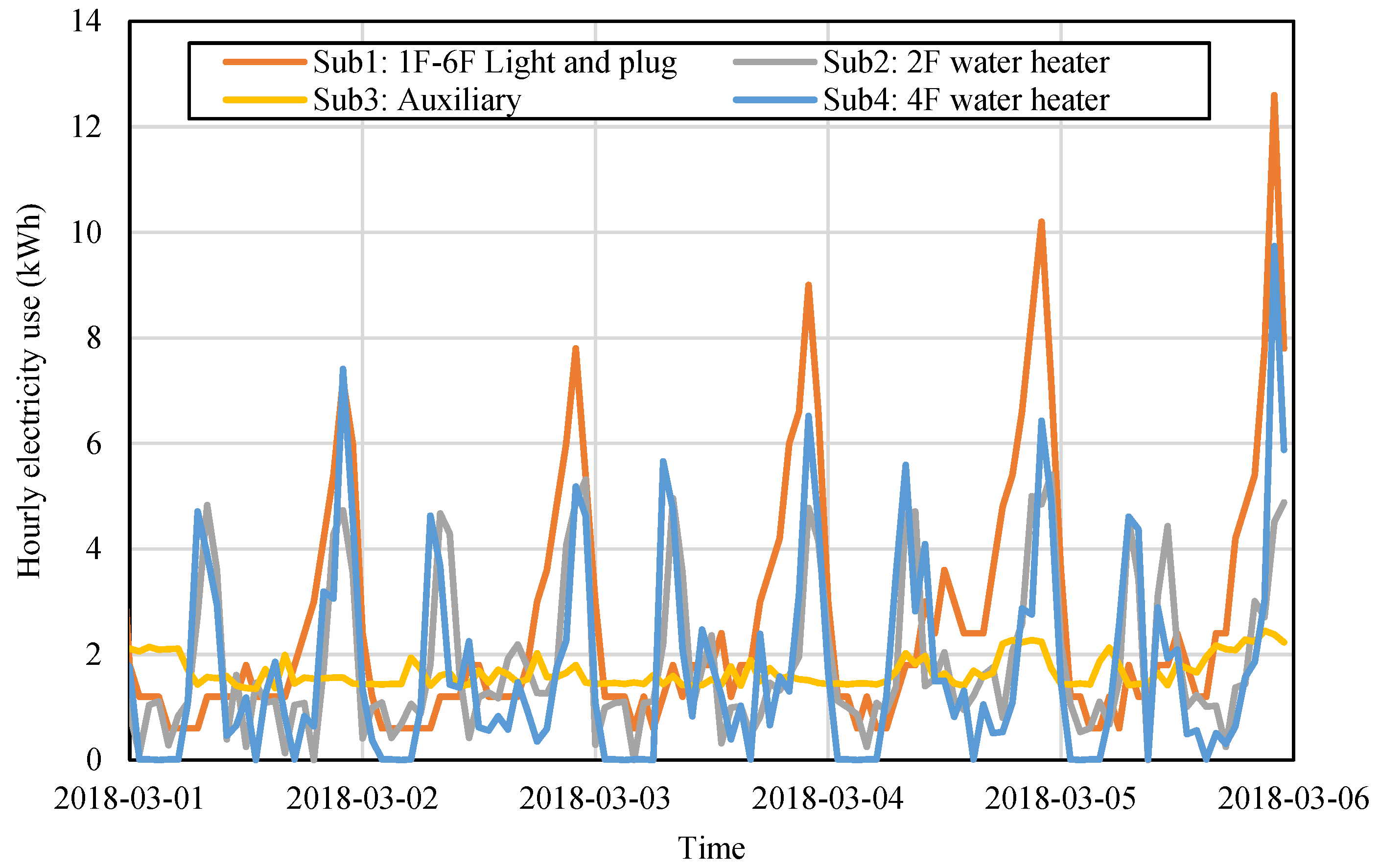
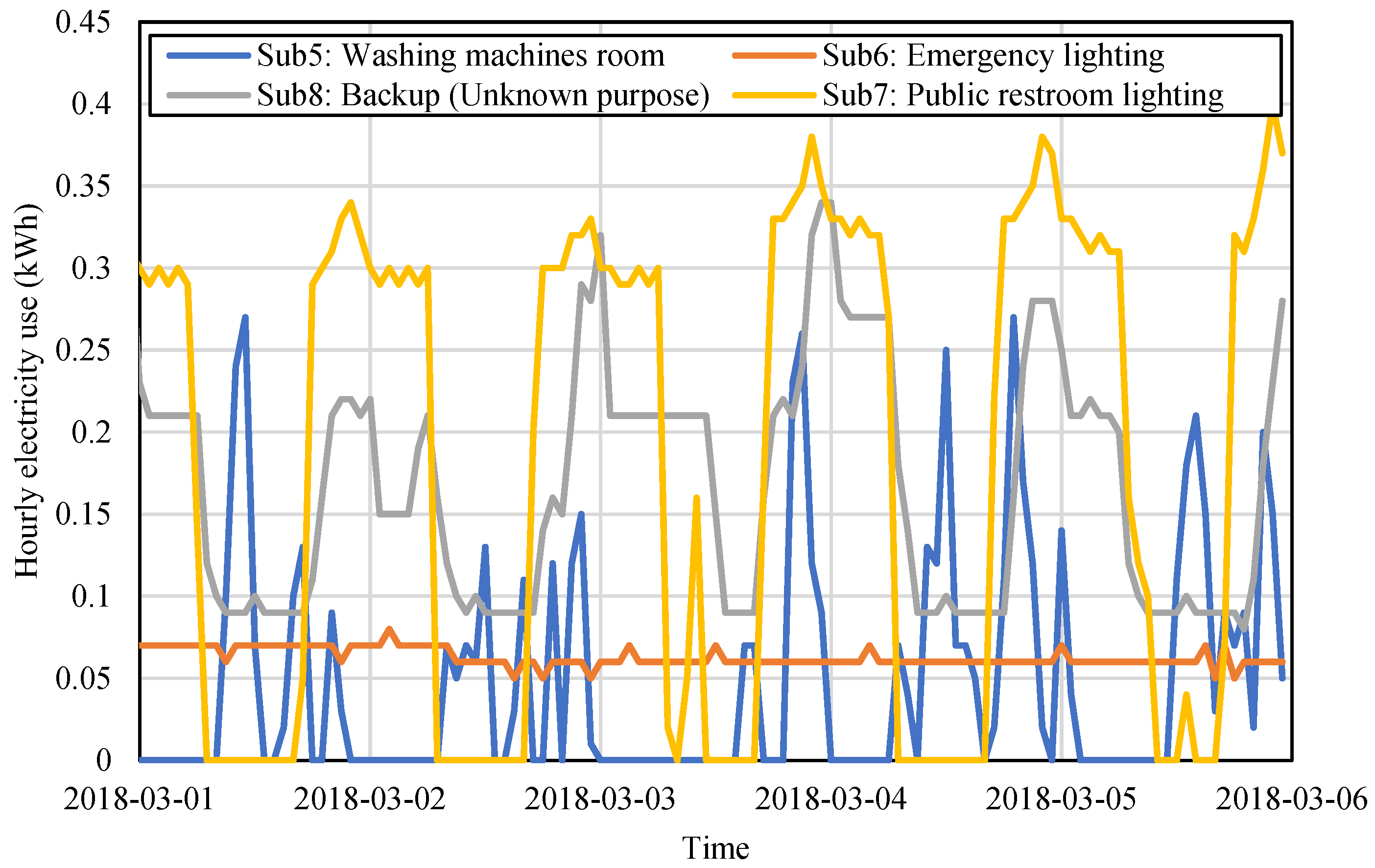
Segments of the time series in Dataset #1 are shown in Figure 13 and Figure 14. The eight submeters can be divided into two categories with distinctive fluctuation ranges. The first category consists of Submeters 1 to 4, with hourly usage roughly ranging between 0 and 13 kWh, while the second category consists of Submeters 5 to 8, with hourly usage roughly ranging between 0 and 0.5 kWh.

Figure 13. Examples of the time series of the submeters with higher energy usage level.

Figure 14. Examples of the time series of the submeters with lower energy usage level.

Submeter 1 has only one peak in a day, which occurs around 22:00, while the two water heaters mainly have two peaks, one in the morning and the other in the evening. Submeter 3 maintains a stable, but relatively lower energy consumption level (around 2 kWh per hour) throughout the entire day. In the second category, the same stable curve can be observed on Submeter 6, with hourly usage no larger than 0.1 kWh. Submeters 7 and 8 have regular nightly usage patterns but with a distinctive daytime usage baseline. Submeter 5 exhibits less regularity with high randomness and significant fluctuations.

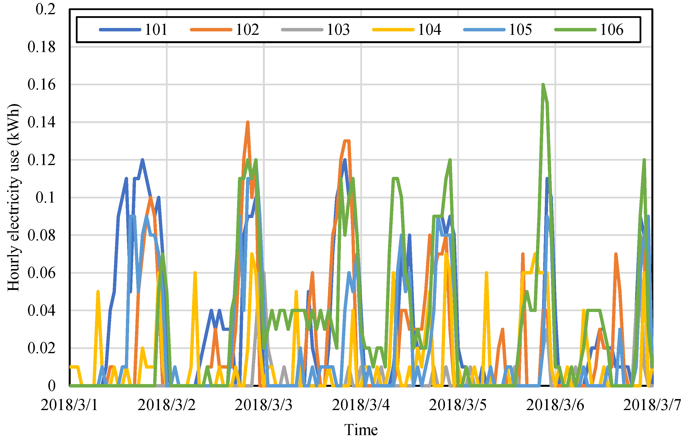
Due to the large number of meters in Dataset #2, segments of the time series of six room meters are chosen and shown in Figure 15. In general, rooms have similar peak levels and nighttime emphasized patterns, but the daily behaviors are extremely inconsistent and change drastically in the week.

Figure 15. Examples of the time series of the room meters in Dataset #2.

4.1.3. Simulation of Time-Deviated Sequences

In each dataset, time deviations with random lengths and positions in each meter’s time series are simulated based on the ground truth data. Firstly, the 5 min granularity time series of all submeters are constructed by randomly dividing the hourly data into twelve parts. Then the hourly values of submeters are added up to simulate a total meter and construct a total-sub node where the law of conservation of energy is strictly satisfied. Thirdly, the cumulative value sequence of each meter can be obtained by the cumulative summation of the hourly value time series.

With the proportion of time deviated data initially set to be 10%, the positions of such data points are chosen randomly within each submeter’s time series, with the first and the last points excluded. To construct the simultaneous time deviations between the total meter and the submeters, whenever one or more submeters have time deviated data in an interval, the total meter is set to also contain such data.

The length of each time deviation is selected randomly within {5, 10, 15, 20, 25, 30} with the unit of minute, and adopts a discrete probability density distribution of {0.2, 0.2, 0.2, 0.2, 0.1, 0.1}. The probability distribution is set to be more exaggerated than the actual situation to make the correction results more prominent.

4.1.4. Performance Evaluation Setup

(1) Correction performance evaluation metrics

To test the time deviation correction performance, in each dataset, all the simulated time-deviated sequences of cumulative energy consumption values are synchronized with the proposed method and methods for comparison. Then the corrected sequences are compared with the corresponding ground truth sequences with RMSE and MAE on positions where time deviation occurs. The equations of the metrics are given below.

$$\mathrm{RMSE}=\sqrt{{\displaystyle \frac{1}{n}}{\sum }_{i=1}^n{\left(E_i-{\widehat{E}}_i\right)}^2}$$

(27)

$$\mathrm{MAE}={\displaystyle \frac{{\sum }_{i=1}^n\left|E_i-{\widehat{E}}_i\right|}{n}}$$

(28)

where E_i is the true value, ${\widehat{E}}_i$ is the correction value, $\overline{E}$ is the mean of the true values, and n is the total number of correction values.

(2) Scalability evaluation setup

The method’s scalability on different numbers of submeters is tested within both Dataset #1 and Dataset #2 with increasing numbers of used submeters starting with 4. For Dataset #1 with eight submeters, one submeter is added each time, and for Dataset #2, two submeters are added each time. The specific submeters used for each scenario are summarized in Table 4.

Table 4. Submeter configurations for scalability test.

Dataset	Total Number of Submeters Used	Names of Used Submeters
#1	4	Sub1, Sub2, Sub3, Sub4
	5	Sub1, Sub2, Sub3, Sub4, Sub5
	6	Sub1, Sub2, Sub3, Sub4, Sub5, Sub6
	7	Sub1, Sub2, Sub3, Sub4, Sub5, Sub6, Sub7
	8	Sub1, Sub2, Sub3, Sub4, Sub5, Sub6, Sub7, Sub8
#2	4	101, 102, 103, 104
	6	101, 102, 103, 104, 105, 106
	8	101, 102, 103, 104, 105, 106, 108, 109
	10	101, 102, 103, 104, 105, 106, 108, 109, 110, 111
	12	101, 102, 103, 104, 105, 106, 108, 109, 110, 111, 112, 113
	14	101, 102, 103, 104, 105, 106, 108, 109, 110, 111, 112, 113, 114, 115
	16	101, 102, 103, 104, 105, 106, 108, 109, 110, 111, 112, 113, 114, 115, 116, 117
	18	101, 102, 103, 104, 105, 106, 108, 109, 110, 111, 112, 113, 114, 115, 116, 117, 118, 119
	20	101, 102, 103, 104, 105, 106, 108, 109, 110, 111, 112, 113, 114, 115, 116, 117, 118, 119, 120, 121

4.2. Performance Analysis

4.2.1. Overall Correction Performance

As comparisons to the proposed method, other chosen conventional time registration or data fusion methods are:

(1) Linear interpolation, Cubic spline interpolation [39], and Lagrange interpolation [46]. The Lagrange interpolation is implemented with a moving window strategy with a window size of 5 to ensure numerical stability, with the correction target point at the center. Therefore, the three interpolation methods are linear, cubic, and quartic polynomials, respectively. For all interpolation methods, including the A-PCHIP, all interpolation calculations use only original measurement data, with no estimates from previous steps involved.

(2) The weighted least squares (WLS) method. As data fusion problems are highly related to a specific arrangement of sensors, the WLS method is chosen for it is a general-purpose data fusion method and can be applied to the problem of this study. In each dataset consisting of one total meter and multiple submeters, it is executed on each cross-sectional data slice of all meters’ time series where abnormal data exists. Only abnormal data points in each time slice are adjusted by the weighted least square strategy so that all data points in the slice conform to the law of energy conservation. The weights are set to be inversely proportional to corresponding hourly electricity consumption values, for the purpose that higher electricity consumption values, with greater possibilities of resulting in larger numerical deviations under the condition that the time deviations follow the same probability distribution, receive greater adjustments to their electricity consumption values.

The RMSE and MAE results of all nine meters originated from Dataset #1 before and after the deviation correction are shown in Table 5 and Table 6, respectively. The energy consumption level and fluctuation characteristics of each meter are different; thus, the performances of each method across all nine meters are Min-Max normalized into the [0,1] interval.

Table 5. RMSE before and after the deviation correction (Unit: kWh).

Method	Total Meter	Sub 1	Sub 2	Sub 3	Sub 4	Sub 5	Sub 6	Sub 7	Sub 8	Normalized Mean
Unsynchronized	3.095	1.228	0.845	0.551	0.981	0.040	0.018	0.059	0.073	-
WLS	1.153	1.573	1.146	0.831	1.302	0.069	0.032	0.093	0.114	0.923
Lagrange	0.949	0.519	0.316	0.200	0.373	0.015	0.007	0.022	0.022	0.082
Linear	0.939	0.458	0.357	0.108	0.539	0.021	0.004	0.017	0.017	0.073
Cubic Spline	0.686	0.464	0.308	0.139	0.355	0.017	0.005	0.018	0.016	0.036
A-PCHIP-iKF	0.305	0.416	0.294	0.126	0.358	0.017	0.005	0.017	0.015	0.010

Table 6. MAE before and after the deviation correction (Unit: kWh).

Method	Total Meter	Sub 1	Sub 2	Sub 3	Sub 4	Sub 5	Sub 6	Sub 7	Sub 8	Normalized Mean
Unsynchronized	2.390	0.825	0.593	0.471	0.572	0.023	0.015	0.042	0.045	-
WLS	0.677	1.149	0.871	0.748	0.808	0.041	0.029	0.073	0.075	0.914
Lagrange	0.643	0.312	0.234	0.145	0.245	0.010	0.005	0.016	0.016	0.077
Linear	0.623	0.277	0.263	0.087	0.346	0.014	0.003	0.012	0.009	0.071
Cubic Spline	0.464	0.265	0.221	0.109	0.232	0.011	0.004	0.013	0.010	0.033
A-PCHIP-iKF	0.187	0.247	0.209	0.101	0.237	0.011	0.004	0.012	0.009	0.009

The proposed method exhibited the best performance compared to other methods in terms of both the normalized mean RMSE (0.010 kWh) and MAE (0.009 kWh) metrics on the nine meters exhibiting different energy consumption characteristics, followed by the Cubic Spline, Linear interpolation, and Lagrange interpolation. The WLS method exhibited the worst overall performance: although it reduced the deviations on the submeter and achieved comparable results with other methods, the deviations of the submeters were all enlarged, indicating that the correction values converged to positions even further from the true values.

The best correction accuracy of each submeter is delivered by different methods. For example, the Cubic Spline performed the best on Submeter 4 in terms of both metrics, and a similar scenario can be observed on Submeters 3, 6, and 7 with the Linear interpolation.

Despite the different performances on specific submeters, the A-PCHIP-iKF provided the best performance on the total meter with RMSE of 0.305 kWh and MAE of 0.187 kWh, which outperformed the second-best method, Cubic Spline, with 56% RMSE and 60% MAE improvements. As discussed in Section 2.3, the total meter of the building has the greatest significance in maintaining high data accuracy. Results showed that the A-PCHIP-iKF method has proved effective in delivering the best correction performance on the total meter.

4.2.2. Scalability on Different Numbers of Submeters

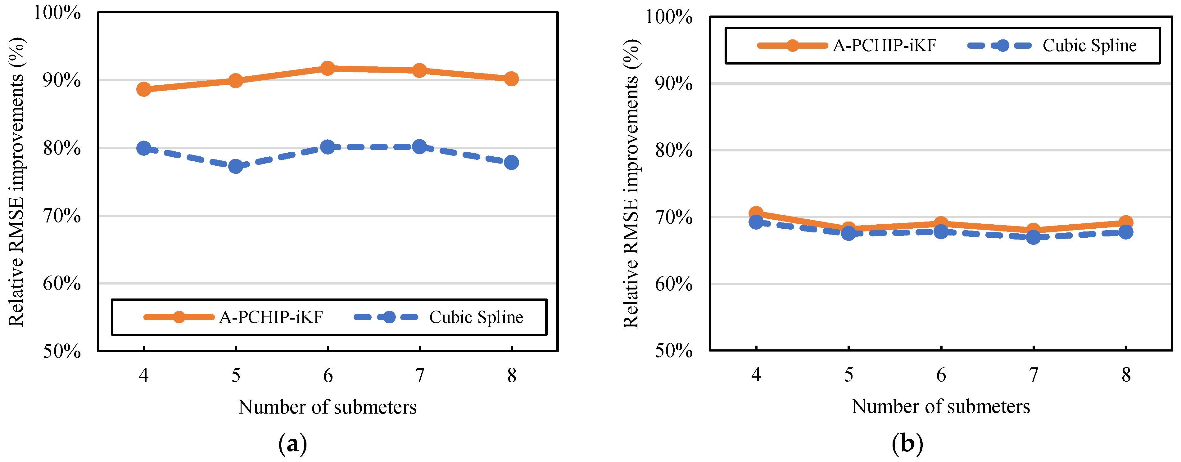
The scalability results of the proposed method and the Cubic Spline interpolation on each dataset are shown in Figure 16 and Figure 17, respectively. As the ground truth sequences of the total meters are simulated by adding up those of the submeters, with different numbers of total submeters, the ground truth sequences of the total meters are also inconsistent. Therefore, the relative improvements between the corrected sequences and the unsynchronized ones in terms of RMSE are used as the evaluation metric. The relative improvements on the total meter and the average relative improvements on the submeters in Dataset #1 are shown in Figure 16a and Figure 16b, respectively. The results of Dataset #2 are shown in Figure 17 with the same setup.

Figure 16. Scalability results of different numbers of submeters in Dataset #1. (a) Relative improvements of the total meter; (b) average relative improvements of submeters.

Figure 17. Scalability results of different numbers of submeters in Dataset #2. (a) Relative improvements of the total meter; (b) average relative improvements of submeters.

The proposed method exhibited sufficient scalability in both datasets with different configurations of submeters. Although the specific patterns on the two datasets are slightly different due to the submeters’ diverse energy consumption characteristics, the proposed method’s relative correction performance is generally stable with the increased number of used submeters.

Firstly, in Dataset #1, with the number of submeters increased, the relative correction improvement of the proposed method on the total meter slightly increased from 89% to 92% and then slightly decreased to 90%, with the turning point occurring at a total of 6 submeters. The average correction improvement on submeters overall remained stable at around 69%. Compared with the Cubic Spline method, the proposed method consistently maintained a lead of at least 9% on the total meter and an average lead of 1% on the submeters.

In Dataset #2, the relative correction improvement of the proposed method on the total meter increased from 86% to 94% as the number of submeters accumulated from 4 to 12, then with more submeters added, the relative improvement remained stable at around 94%–95%. The relative correction improvement of the Cubic Spline method exhibited a trend of increasing first and then decreasing as the number of partitions increases. The dividing point is around 14 to 16 submeters. In general, the proposed method demonstrated a more stable trend and consistently maintained a lead of around 10% on the total meter, under the conditions that the two methods’ average performances on submeters were almost identical.

4.2.3. Adaptive PCHIP Improvements and Parameter Sensitivity Analysis

The RMSE and MAE results of standard PCHIP and the proposed A-PCHIP are shown in Table 7. Apart from the non-improvement on Submeter 3, the A-PCHIP exhibited 0.53% to 5.62% improvements compared to the standard counterpart, with the max improvements observed on Submeter 4 with 5.62% RMSE and 5.33% MAE, followed by 2.77% and 2.52% improvements on the total meter, and around 2% on Submeter 1 and 2 in terms of RMSE. For Submeter 5 to 8 in Dataset #1 and all submeters in Dataset #2, A-PCHIP exhibited negligible improvements similar to Submeter 3, and thus the results of these meters are omitted. Possible reasons are low energy consumption levels or limited fluctuation ranges, in which case the cumulative energy curve is more likely to manifest a nearly linear growth, and the improvement brought by parameter optimization is limited.

Table 7. Comparison between standard PCHIP and A-PCHIP.

Method	Metrics	Total Meter	Submeter 1	Submeter 2	Submeter 3	Submeter 4
Standard	RMSE (kWh)	0.697	0.339	0.268	0.116	0.423
	MAE (kWh)	0.468	0.209	0.183	0.091	0.231
Adaptive	RMSE (kWh)	0.677	0.333	0.262	0.116	0.399
	MAE (kWh)	0.456	0.208	0.179	0.091	0.219
Relative improvements	RMSE (%)	2.77%	1.77%	1.98%	0.00%	5.62%
	MAE (%)	2.52%	0.53%	2.13%	0.00%	5.33%

To study the impact of the weight coefficient ranges of the A-PCHIP method on the correction performance, the relative RMSE improvements compared with the standard PCHIP on the five meters with different ranges of the coefficients were tested, with 0.1 as the fixed lower limit and the upper limit ranging from 1 to 100. The optimal parameters of all meters are listed in Table 8. As the initial parameters start with the {2.0, 1.0} as the standard PCHIP, the meter with a larger optimal parameter takes longer searching time.

Table 8. Optimal parameters of meters with A-PCHIP.

	Total Meter	Submeter 1	Submeter 2	Submeter 3	Submeter 4
Optimal α1	80.56	36.52	14.97	1.23	39.21
Optimal α2	0.1	0.1	0.1	0.1	0.1
Total time used (s)	6.73 s	5.46 s	4.36 s	1.83 s	5.78 s

The parameter sensitivity analysis of the total meter is shown in Figure 18. As the upper limit increased from 1 to 50, the optimized α₁ consistently reached the respective upper limit. The optimized α₁ finally stopped at 80.6 when the limit was further extended to 100 or larger, while the optimal result of α₂ consistently equaled 0.1.

Figure 18. Relative RMSE improvements compared with the standard PCHIP on the total meter.

The parameter sensitivity of the correction effect is low when the upper limit is larger than 5. As the upper limit increased from 5 to 50, the total time used for optimization increased linearly, but the increment of the relative improvement was slow, with an overall growth of 0.14%. Therefore, the optimal parameter does not have to be reached to achieve satisfactory performance. If the best performance is preferred, the upper limit can be set to 30, which can yield just as good performance as the finalized optimal parameters with 17% shorter time consumption. If computational efficiency is preferred, setting the upper limit to 5 can bring satisfactory results with almost 48% less time consumption.

4.2.4. The Impact of the Proportion of Abnormal Data

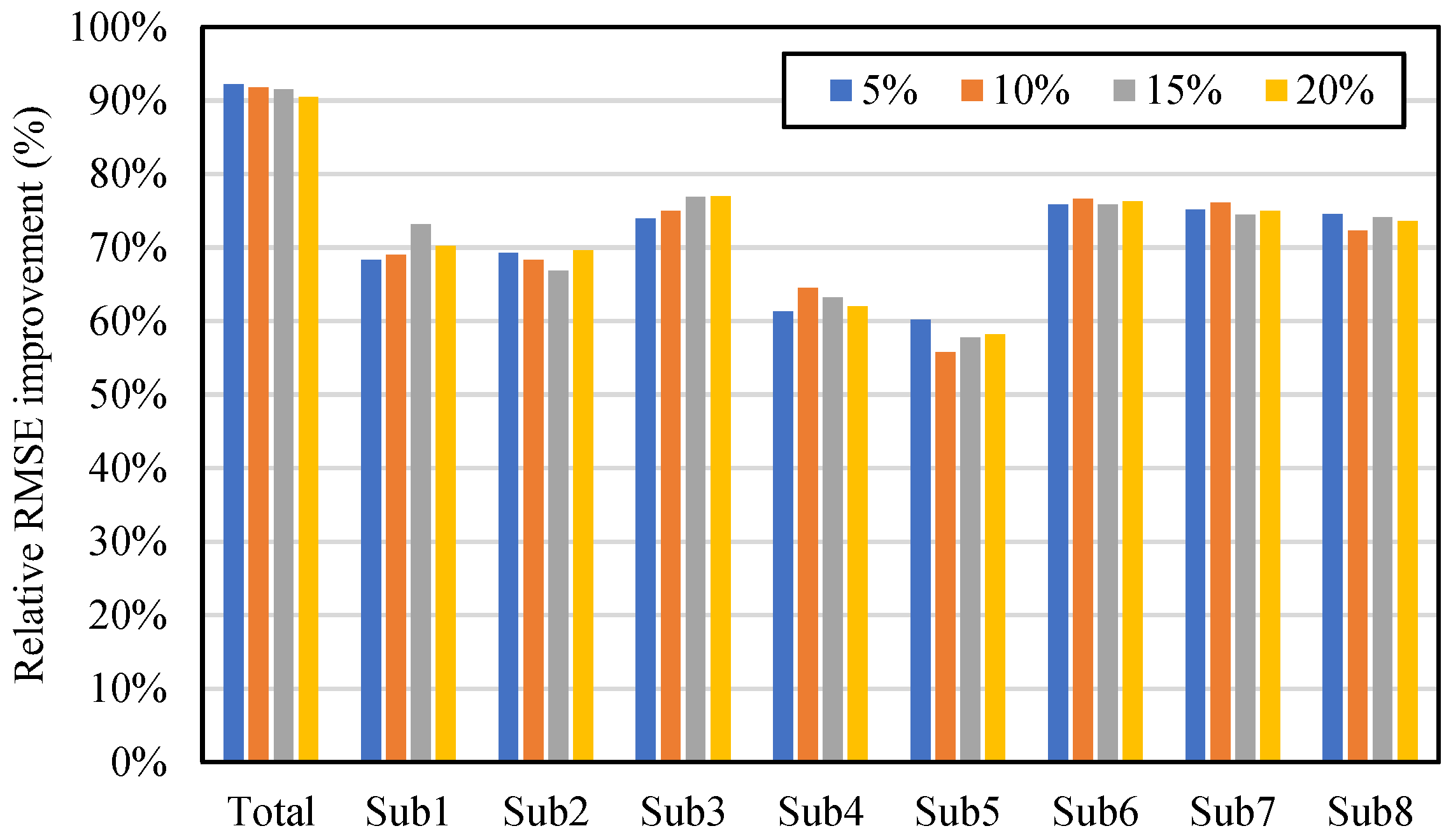
The impact of different proportions of abnormal data is studied by setting the abnormal data proportion of the eight submeters in Dataset #1 to 5%, 10%, 15% and 20% in the data simulation process. As the instances of abnormal data in the ground truth sequences of the total meter are the union of randomly distributed abnormal instances of the submeters, the corresponding resulting proportions of abnormal data of the total meter are 33.5%, 58.5%, 71.7% and 83.2%. As a reference, the average abnormal proportions of real data analyzed in Section 2.2 are about 10% per meter.

Results are shown in Figure 19 in terms of the relative RMSE improvement. The impact was insignificant as the abnormal proportion increased, as the relative RMSE improvements of each meter did not exhibit obvious regularity. This is primarily contributed by the independence of the correction process of the A-PCHIP at each time a deviated data point, which does not involve any estimated data and only utilizes original data that has high measuring and temporal accuracy.

Figure 19. Relative RMSE improvements with different proportions of abnormal data.

4.2.5. Computational Complexity Analysis

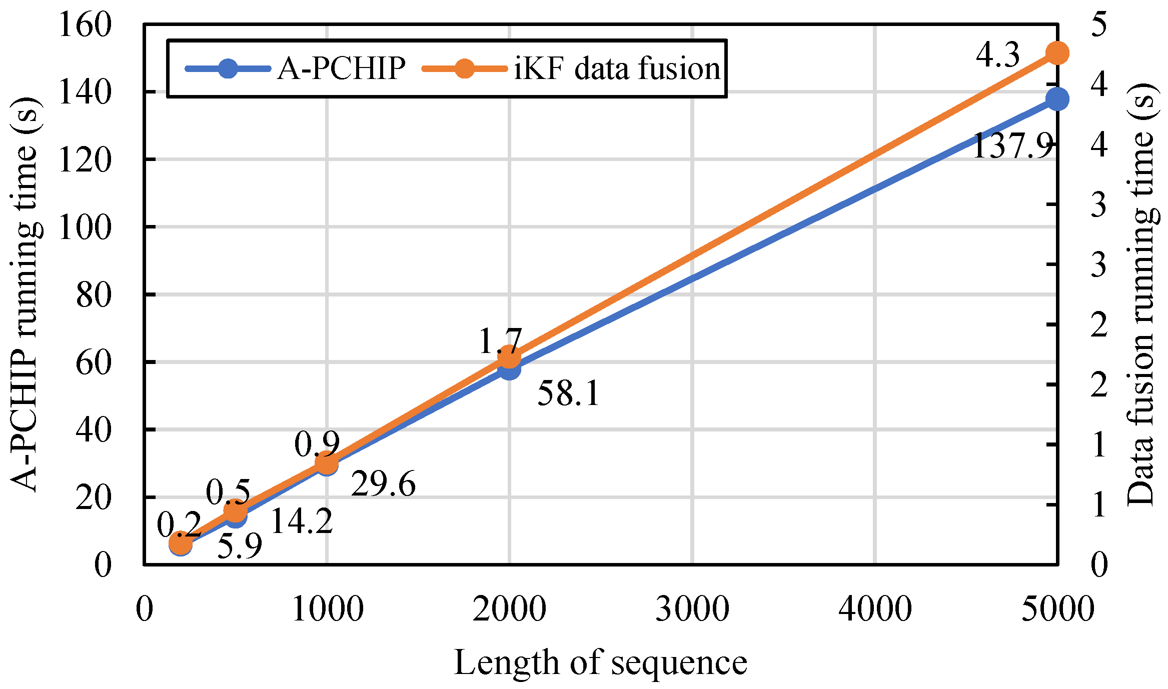
The A-PCHIP interpolation mainly consists of two processes that are parameter optimization and prediction, and the former includes k calculations of the LOOCV loss function, where k represents the number of iterations for optimization. The time complexity of the calculation of the loss function and the prediction process is O(n). Therefore, the total time complexity of the A-PCHIP is O(n). The time complexity of iKF data fusion is also O(n) for each meter.

The methods are tested on a computer with an Intel Core i5 CPU and 16 GB of RAM with Python 3.10. The eight submeters of Dataset #1 are chosen as correction subjects, and different lengths of energy data sequences are simulated. Each sequence length is tested four times with high-res ground truth sequences generated twice, where random positions are chosen twice, and the average running time is calculated. The results are summarized in Table 9, and the relationship between running time and length of sequence is shown in Figure 20. The running time of the methods is both linearly related to the length of the sequence. In practical applications, the hourly energy data sequences can be segmented by week or month, which can restrict the sequence length and enhance parallel computing efficiency.

Table 9. Average running time of A-PCHIP and iKF.

Length of Sequence n	A-PCHIP Running Time (s)	T(n)/n	iKF Running Time (s)	T(n)/n
100	2.7 s	2.7 × 10−2	0.1 s	1.0 × 10−3
200	5.9 s	3.0 × 10−2	0.2 s	9.0 × 10−4
500	14.2 s	2.8 × 10−2	0.5 s	9.0 × 10−4
1000	29.6 s	3.0 × 10−2	0.9 s	8.5 × 10−4
2000	58.1 s	2.9 × 10−2	1.7 s	8.7 × 10−4
5000	137.9 s	2.8 × 10−2	4.3 s	8.5 × 10−4

Figure 20. Running time of the methods with different lengths of data sequence.

4.2.6. Practical Benefit Analysis

In practice, the deviation of energy consumption values will have an impact on the periodic billing results [67,68]. In this study, time deviations primarily affect the numerical accuracy of the hourly data. Therefore, the time-of-use electricity pricing scenario is considered, and the costs of deviated and corrected electricity consumption data of the sample building are calculated, based on the simulated temporally deviated data and corrected data by the proposed method. The time-of-use electricity pricing data are retrieved from the open-source Open Power System Data [69]. Costs in a year are shown in Table 10, with January and February excluded due to low energy consumption and long periods of data missing that are likely to be caused by the winter vacation. Due to the time deviation, the deviated costs were mostly smaller than the true costs in the ten months, causing a total of -0.185% relative error in the year. After data correction by the proposed method, the relative errors of the costs are greatly reduced, with a total of 0.002% in the year.

Table 10. Costs of deviated and corrected electricity consumption data.

Month	True Costs (£)	Deviated Costs (£)	Deviated Relative Error (%)	Corrected Costs (£)	Corrected Relative Error (%)
March	409.78	408.27	−0.369%	409.87	0.023%
April	357.52	357.07	−0.124%	357.50	−0.004%
May	342.32	341.26	−0.308%	342.26	−0.016%
June	255.70	255.51	−0.071%	255.67	−0.011%
July	110.92	111.12	0.182%	110.95	0.031%
August	75.97	75.93	−0.055%	75.97	0.000%
September	342.66	342.26	−0.116%	342.71	0.014%
October	423.32	422.30	−0.241%	423.32	0.000%
November	419.25	418.55	−0.167%	419.26	0.003%
December	501.39	500.56	−0.166%	501.36	−0.006%
Total	3238.81	3232.83	−0.185%	3238.88	0.002%

4.2.7. Correction Stability and Data Consistency After Correction

The monotonicity-preserving ability of interpolation methods is important for circuits whose energy consumption rate can be zero during idle hours. Correction stability is evaluated by counting the total number of negative hourly energy usage values after deviation correction on meters in Dataset #1, which indicates the method’s ability to consistently provide physically meaningful results, especially on submeters like Submeter 2, 4, 5, and 7, whose cumulative energy consumption value can remain unchanged for several hours. The results are shown in Table 11.

Table 11. Correction stability by count of negative hourly values generated.

Method	Count of Negative Hourly Values
Unsynchronized	0
WLS	9
Lagrange	10
Linear	0
Cubic Spline	11
A-PCHIP-iKF	5

For all tested methods, all negative values are contributed by the above-mentioned submeters that can exhibit consecutive zero hourly values. Negative hourly values do not conform to physical laws and require additional corrections. The proposed A-PCHIP-iKF method does not generate negative values during the time registration procedure, but it may generate a few negative values during the data fusion process. Despite this, the proposed method still produces the least negative values compared to the Lagrange and Cubic interpolation. Therefore, its impact on the overall correction performance is the smallest.

Table 12 gives the data consistency between the total meter and the submeters before and after deviation correction, which is measured by the standard deviation of the total-sub difference. Results showed that data consistency can be improved by all methods, indicating the positive effect of data correction. Although the WLS method provided absolute consistent results, its poor performance of the correction effect on all meters makes it lack usability. Among other methods, the proposed method exhibited a distinguishing performance with a standard deviation of 0.152 kWh, with a 71.6% improvement compared to the 0.537 kWh of the second-best method.

Table 12. Data consistency between the total meter and the submeters.

Method	Data Consistency (kWh)
Unsynchronized	1.789
WLS	0.000
Lagrange	0.762
Linear	0.629
Cubic Spline	0.537
A-PCHIP-iKF	0.152

4.3. Discussion

4.3.1. Contributions

This paper points out the issue of time deviations in building electricity consumption data, which has been overlooked in existing research regarding building energy data. Time deviations can have great impacts on the numerical accuracy of building energy data. They are prone to being neglected as they originated from the process where the temporal information is initially attached, and they can only be identified by methods like comparing the data consistency between the total meter and the submeters or using the data collection status codes. Therefore, it is necessary to study their causes and characteristics and provide mitigation methods.

The A-PCHIP-iKF method proposed in this paper effectively addresses the issues regarding continuous time delay and monotonicity constraints, which existing methods cannot resolve. The existing asynchronous data fusion methods have limitations, such as the specific requirements for the sampling period, or are based on the assumption of delay discretization, and thus cannot be directly applied to the correction of continuous time deviations of building energy consumption data. Besides, the existing spline interpolation has also been proven to be unable to effectively address the monotonicity constraint of cumulative energy consumption data in this paper. The A-PCHIP-iKF method effectively combines the advantages of time registration and data fusion methods. It can utilize the temporal and spatial correlation of multiple correlated time series to improve the numerical accuracy of corrected data of the total meter, which makes its deviation-calibrating performance more advantageous. In addition, the method can be applied directly to data sequences that contain time deviated data and does not require feature learning with continuous error-free historical data, like other statistical and machine learning methods, which makes it especially suitable for the time deviation correction problem.

Finally, the A-PCHIP-iKF method demonstrates a significant performance improvement compared to existing methods, especially on the correction of the building total meter. By improving the calculation process of the weight parameters, it can adaptively adjust the parameters based on the actual data characteristics, achieving up to 5.62% improvement in correction effect compared to the standard PCHIP. Moreover, the A-PCHIP-iKF method establishes a virtual meter model based on energy conservation and performs iterative data fusion using iKF, which can further enhance the correction effect of the total meter by utilizing sub-meters’ data. Compared to traditional methods, the effect of A-PCHIP-iKF on the building’s total meter is notably improved with an RMSE improvement of 56% and an MAE improvement of 60%.

4.3.2. Scalability on Other Types of Energy Data

The A-PCHIP relies on the assumption that the variation of physical quantities has short-term temporal regularity. It utilizes the local patterns of the data curve to provide smooth interpolation results. Compared with other commonly used interpolation algorithms, its advantage lies in that its derivative setting logic can avoid overshoot or oscillation, which is particularly applicable to energy consumption data that sometimes fluctuate and sometimes remain constant, including electricity consumption, heat energy, natural gas, etc. Such characteristics can effectively prevent the Runge phenomenon (local overfitting) and generate interpolation results that do not conform to physical laws. This also makes it applicable to interpolation problems of instantaneous values, such as environmental parameters. In addition, the A-PCHIP introduces adaptive parameter optimization based on the standard method, which can provide optimal parameters and, therefore, better fitting results.

Data fusion usually requires at least two sources of data of the same target. In this paper, additional data from the electricity meter is provided by other related meters based on the law of conservation of energy. For other types of energy data, the key is to find other data sources to provide redundant information. These can either be direct data sources, such as measurement data from redundant sensors, bill data, etc., or data derived from a model, such as time series prediction models, physical models, spatial interpolation models for temperature fields, etc. Most model-based methods attempt to model the temporal or spatial correlation between multiple sensors, so they are usually strongly connected to specific sensor setups. After gaining reliable multisource data, centralized fusion directly targeting measurement values can be carried out as in this paper, or distributed fusion can be conducted as in some literature. The Kalman filter is a simple but efficient dynamic system optimal estimation algorithm with strong noise processing and data fusion capabilities. More importantly, it has strong customization potential in that the specific data fusion logic can be modified according to specific sensor settings to achieve the expected purpose and better results. Based on the experiment results that the proposed method has satisfactory scalability on different numbers of submeters, we believe it can have great potential for other types of energy data.

4.3.3. Real-World Implementation Challenges and Future Directions

Real-world implementation challenges mainly come from the uncertainty of the preconditions.

Firstly, the implementation of the time registration method in this paper is based on the assumption of known, accurate data collection time, which cannot be met in the current circumstances. This requires the improvement of the timestamping mechanism of the data collector by attaching each collected data point with an exclusive and accurate timestamp, which we believe is feasible and necessary. Only by this can the temporally deviated data points be located accurately on the time axis and be effectively utilized for performing time registration.

Secondly, data fusion requires a total meter and submeters that satisfy the energy conservation relationship, which is not universally applicable. Incomplete sub-metering and systematic errors of meters can greatly restrict the application of data fusion methods.

Future directions are as follows.

The optimized parameters of the A-PCHIP are a global optimum in this study, which not only lacks local fitting capability but also limits the online application capability of the proposed method. It can be improved by obtaining the local optimal parameters by using the moving window strategy.

Negative correction value, which is introduced in the data fusion process, cannot be completely avoided. Further theoretical improvements by setting constraints when implementing the KF are needed to avoid the production of negative values. In addition, nonlinear filters like the extended Kalman filter (EKF) can be employed to better match the nonlinear characteristics of building energy consumption data.

The time deviations of normally collected measurements are assumed to be zero in the performance simulation. However, normal data can suffer from small time deviations and other measuring error factors (Figure 6) that may bring instability to deviation correction methods, which need to be validated with more practical situations for constructing test data sets.

5. Conclusions

Time deviations are found in the timestamps of data from a building energy consumption monitoring system, which are caused jointly by the collection failure phenomenon and the flawed timestamping mechanism of the data collector. They can result in the asynchronism of the energy time series, leading to overestimation or underestimation of the spatial and temporal correlation of multi-source data and causing misleading results and conclusions. To correct the time deviations, the A-PCHIP-iKF method is proposed. It includes the time registration for the temporally deviated measurements of each meter’s time series, utilizing the temporal correlations, and the data fusion of multiple spatially correlated time series to achieve the optimum estimation accuracy of all time series simultaneously.

The results showed that the proposed method has significant advantages over traditional methods in terms of correction accuracy, with 56% RMSE and 60% MAE improvements on the total meter of the building. On submeters with diverse characteristics, the method also exhibited the best overall performance according to the normalized metrics. In terms of correction stability on submeters with continuous zero hourly consumption values, the method produced much less negative hourly usage values compared to other methods. Due to the introduction of data fusion, the method provided the best data consistency results between the total meter and the submeters. In conclusion, the proposed A-PCHIP-iKF method achieved a balance between the correction accuracy, stability, and consistency.

References

- Buildings—Energy System—IEA. Available online: https://www.iea.org/reports/buildings (accessed on 30 October 2025).
- Hernández, J.L.; de Miguel, I.; Vélez, F.; Vasallo, A. Challenges and Opportunities in European Smart Buildings Energy Management: A Critical Review. Renew. Sustain. Energy Rev. 2024, 199, 114472. [Google Scholar] [CrossRef]
- Mirzabeigi, S.; Soltanian-Zadeh, S.; Krietemeyer, B.; Dong, B.; Zhang, J. “Jensen” Energy Consumption and IEQ Monitoring in Two University Apartment Buildings: Pre-Retrofit Dataset. Sci. Data 2025, 12, 1022. [Google Scholar] [CrossRef]
- Liu, X.; Ding, Y.; Tang, H.; Xiao, F. A Data Mining-Based Framework for the Identification of Daily Electricity Usage Patterns and Anomaly Detection in Building Electricity Consumption Data. Energy Build. 2021, 231, 110601. [Google Scholar] [CrossRef]
- Hossain, J.; Kadir, A.F.A.; Hanafi, A.N.; Shareef, H.; Khatib, T.; Baharin, K.A.; Sulaima, M.F. A Review on Optimal Energy Management in Commercial Buildings. Energies 2023, 16, 1609. [Google Scholar] [CrossRef]
- Zhu, X.; Zhang, X.; Gong, P.; Li, Y. A Review of Distributed Energy System Optimization for Building Decarbonization. J. Build. Eng. 2023, 73, 106735. [Google Scholar] [CrossRef]
- Liu, J.; Zhang, Q.; Li, X.; Li, G.; Liu, Z.; Xie, Y.; Li, K.; Liu, B. Transfer Learning-Based Strategies for Fault Diagnosis in Building Energy Systems. Energy Build. 2021, 250, 111256. [Google Scholar] [CrossRef]
- Melgaard, S.P.; Andersen, K.H.; Marszal-Pomianowska, A.; Jensen, R.L.; Heiselberg, P.K. Fault Detection and Diagnosis Encyclopedia for Building Systems: A Systematic Review. Energies 2022, 15, 4366. [Google Scholar] [CrossRef]
- Ekström, T.; Burke, S.; Wiktorsson, M.; Hassanie, S.; Harderup, L.-E.; Arfvidsson, J. Evaluating the Impact of Data Quality on the Accuracy of the Predicted Energy Performance for a Fixed Building Design Using Probabilistic Energy Performance Simulations and Uncertainty Analysis. Energy Build. 2021, 249, 111205. [Google Scholar] [CrossRef]
- Iyer, M.; Kumar, S.; Mathew, P.; Mathew, S.; Stratton, H.; Singh, M. Commercial Buildings Energy Data Framework for India: An Exploratory Study. Energy Effic. 2021, 14, 67. [Google Scholar] [CrossRef]
- Zhang, L.; Leach, M. Evaluate the Impact of Sensor Accuracy on Model Performance in Data-Driven Building Fault Detection and Diagnostics Using Monte Carlo Simulation. Build. Simul. 2022, 15, 769–778. [Google Scholar] [CrossRef]
- Li, D.; Wang, Y.; Wang, J.; Wang, C.; Duan, Y. Recent Advances in Sensor Fault Diagnosis: A Review. Sens. Actuators Phys. 2020, 309, 111990. [Google Scholar] [CrossRef]
- Zhang, B.; Rezgui, Y.; Luo, Z.; Zhao, T. Fault Detection Research on Novel Transfer Learning-Based Method for Cross-Condition, Cross-System and Cross-Operation in Public Building HVAC Sensors. Energy 2024, 313, 133704. [Google Scholar] [CrossRef]
- Okafor, N.U.; Alghorani, Y.; Delaney, D.T. Improving Data Quality of Low-Cost IoT Sensors in Environmental Monitoring Networks Using Data Fusion and Machine Learning Approach. ICT Express 2020, 6, 220–228. [Google Scholar] [CrossRef]
- Yang, A.; Wang, P.; Yang, H. In Situ Blind Calibration of Sensor Networks for Infrastructure Monitoring. IEEE Sens. J. 2021, 21, 24274–24284. [Google Scholar] [CrossRef]
- Koo, J.; Yoon, S. In-Situ Sensor Virtualization and Calibration in Building Systems. Appl. Energy 2022, 325, 119864. [Google Scholar] [CrossRef]
- Choi, Y.; Yoon, S.; Park, C.-Y.; Lee, K.-C. In-Situ Observation and Calibration in Building Digitalization: Comparison of Intrusive and Nonintrusive Approaches. Autom. Constr. 2023, 145, 104648. [Google Scholar] [CrossRef]
- Yu, D.; Xia, Y.; Li, L.; Xing, Z.; Zhu, C. Distributed Covariance Intersection Fusion Estimation With Delayed Measurements and Unknown Inputs. IEEE Trans. Syst. Man Cybern. Syst. 2021, 51, 5165–5173. [Google Scholar] [CrossRef]
- Lee, K.; Johnson, E.N. Latency Compensated Visual-Inertial Odometry for Agile Autonomous Flight. Sensors 2020, 20, 2209. [Google Scholar] [CrossRef]
- Chen, B.; Ho, D.W.C.; Hu, G.; Yu, L. Delay-Dependent Distributed Kalman Fusion Estimation With Dimensionality Reduction in Cyber-Physical Systems. IEEE Trans. Cybern. 2022, 52, 13557–13571. [Google Scholar] [CrossRef]
- Wang, K.; Zhang, Q.; Jin, Z.; Fu, X. An Approach to Distributed Asynchronous Multi-Sensor Fusion Utilising Data Compensation Algorithm. IET Radar Sonar Navig. 2025, 19, e12693. [Google Scholar] [CrossRef]
- Hu, Y.; Lin, X. Weighted Average Consensus Filtering for Continuous-Time Linear Systems With Asynchronous Sensor Measurements. IEEE Sens. J. 2025, 25, 6881–6893. [Google Scholar] [CrossRef]
- Shao, T. Distributed Consensus Kalman Filtering for Asynchronous Multi-Rate Sensor Networks. Signal Image Video Process. 2024, 18, 6419–6429. [Google Scholar] [CrossRef]
- Meng, T.; Jing, X.; Yan, Z.; Pedrycz, W. A Survey on Machine Learning for Data Fusion. Inf. Fusion 2020, 57, 115–129. [Google Scholar] [CrossRef]
- Fu, H.; Baltazar, J.-C.; Claridge, D.E. Review of Developments in Whole-Building Statistical Energy Consumption Models for Commercial Buildings. Renew. Sustain. Energy Rev. 2021, 147, 111248. [Google Scholar] [CrossRef]
- Melo, F.C.; Carrilho da Graça, G.; Oliveira Panão, M.J.N. A Review of Annual, Monthly, and Hourly Electricity Use in Buildings. Energy Build. 2023, 293, 113201. [Google Scholar] [CrossRef]
- Liu, H.; Liang, J.; Liu, Y.; Wu, H. A Review of Data-Driven Building Energy Prediction. Buildings 2023, 13, 532. [Google Scholar] [CrossRef]
- Chen, Y.; Guo, M.; Chen, Z.; Chen, Z.; Ji, Y. Physical Energy and Data-Driven Models in Building Energy Prediction: A Review. Energy Rep. 2022, 8, 2656–2671. [Google Scholar] [CrossRef]
- Fathi, S.; Srinivasan, R.; Fenner, A.; Fathi, S. Machine Learning Applications in Urban Building Energy Performance Forecasting: A Systematic Review. Renew. Sustain. Energy Rev. 2020, 133, 110287. [Google Scholar] [CrossRef]
- Martin Nascimento, G.F.; Wurtz, F.; Kuo-Peng, P.; Delinchant, B.; Jhoe Batistela, N. Outlier Detection in Buildings’ Power Consumption Data Using Forecast Error. Energies 2021, 14, 8325. [Google Scholar] [CrossRef]
- Valverde, J.; Cruz, A.; Vaccaro, C.; Luna, J.; Cordova-Garcia, J. Identifying Data Issues in Networked Energy Monitoring Platforms. In Proceedings of the 2024 IEEE International Symposium on Measurements & Networking (M&N), Rome, Italy, 2–5 July 2024; pp. 1–6. [Google Scholar]
- Rusek, R.; Melendez Frigola, J.; Colomer Llinas, J. Influence of Occupant Presence Patterns on Energy Consumption and Its Relation to Comfort: A Case Study Based on Sensor and Crowd-Sensed Data. Energy Sustain. Soc. 2022, 12, 13. [Google Scholar] [CrossRef]
- Lee, J.-Y.; Wargocki, P.; Chan, Y.-H.; Chen, L.; Tham, K.-W. Indoor Environmental Quality, Occupant Satisfaction, and Acute Building-Related Health Symptoms in Green Mark-Certified Compared with Non-Certified Office Buildings. Indoor Air 2019, 29, 112–129. [Google Scholar] [CrossRef] [PubMed]
- Sözer, H.; Aldin, S.S. Predicting the Indoor Thermal Data for Heating Season Based on Short-Term Measurements to Calibrate the Simulation Set-Points. Energy Build. 2019, 202, 109422. [Google Scholar] [CrossRef]
- Hao Chew, B.S.; Xu, Y.; Yuan, D.H. Non Intrusive Load Monitoring for Industrial Chiller Plant System—A Long Short Term Memory Approach. In Proceedings of the 2019 9th International Conference on Power and Energy Systems (ICPES), Perth, WA, Australia, 10–12 December 2019; pp. 1–5. [Google Scholar]
- Wang, J.; Jazizadeh, F. Towards Light Intensity Assisted Non-Intrusive Electricity Disaggregation. In Computing in Civil Engineering 2017; American Society of Civil Engineers: Seattle, WA, USA, 2017; pp. 179–186. [Google Scholar]
- Mitchell, H.B. Data Fusion: Concepts and Ideas; Springer: Berlin/Heidelberg, Germany, 2012; ISBN 978-3-642-27221-9. [Google Scholar]
- Cengiz, B.; Adam, I.Y.; Ozdem, M.; Das, R. A Survey on Data Fusion Approaches in IoT-Based Smart Cities: Smart Applications, Taxonomies, Challenges, and Future Research Directions. Inf. Fusion 2025, 121, 103102. [Google Scholar] [CrossRef]
- Chen, Z.; Bo, Y.; Zhao, W.; Pan, L.; Chen, J. Time Registration Algorithm of Multi Sensors Based on Spline Interpolating. WSEAS Trans. Math. 2017, 16, 143–151. [Google Scholar]
- Kuang, Y.; Lu, Z.; Li, L.; Chen, Z.; Cui, Y.; Wang, F. Robust Constrained Kalman Filter Algorithm Considering Time Registration for GNSS/Acoustic Joint positioning. Appl. Ocean Res. 2021, 107, 102435. [Google Scholar] [CrossRef]
- Arend, J.M.; Pörschmann, C.; Weinzierl, S.; Brinkmann, F. Magnitude-Corrected and Time-Aligned Interpolation of Head-Related Transfer Functions. IEEEACM Trans. Audio Speech Lang. Process. 2023, 31, 3783–3799. [Google Scholar] [CrossRef]
- Zhou, G.; Bu, S.; Kirubarajan, T. Simultaneous Spatiotemporal Bias Compensation and Data Fusion for Asynchronous Multisensor Systems. Chin. J. Inf. Fusion 2024, 1, 16–32. [Google Scholar] [CrossRef]
- Hua, Y.; Wan, F.; Gan, H.; Liao, B. One-Step Asynchronous Data Fusion DLMS Algorithm. IEEE Commun. Lett. 2021, 25, 1660–1664. [Google Scholar] [CrossRef]
- Zhang, K.; Wang, Z.; Guo, L.; Peng, Y.; Zheng, Z. An Asynchronous Data Fusion Algorithm for Target Detection Based on Multi-Sensor Networks. IEEE Access 2020, 8, 59511–59523. [Google Scholar] [CrossRef]
- Hua, Y.; Gan, H.; Wan, F.; Qing, X.; Liu, F. Distributed Estimation With Adaptive Cluster Learning Over Asynchronous Data Fusion. IEEE Trans. Aerosp. Electron. Syst. 2023, 59, 5262–5274. [Google Scholar] [CrossRef]
- Huimin, L.; Tianyi, D.; Jingjing, S.; Hongyang, S.; Xuming, H.; Gang, L. Translation Registration Algorithm for Multi-Source Time Series Data Based on the Sliding Window. J. Eng. Sci. Technol. Rev. 2016, 9, 44–50. [Google Scholar] [CrossRef]
- Qiu, Z.; Martínez-Sánchez, J.; Arias-Sánchez, P.; Rashdi, R. External Multi-Modal Imaging Sensor Calibration for Sensor Fusion: A Review. Inf. Fusion 2023, 97, 101806. [Google Scholar] [CrossRef]
- Zhu, G.; Zhou, F.; Xie, L.; Jiang, R.; Chen, Y. Sequential Asynchronous Filters for Target Tracking in Wireless Sensor Networks. IEEE Sens. J. 2014, 14, 3174–3182. [Google Scholar] [CrossRef]
- Wang, X.; Chen, K.; Wang, M.; Xue, Q. Time Registration Algorithm Based on Multi-Missiles Cooperative Target Detection. In Proceedings of the 2019 IEEE International Conference on Unmanned Systems and Artificial Intelligence (ICUSAI), Xi’an, China, 22–24 November 2019; pp. 75–79. [Google Scholar]
- Blair, W.D.; Rice, T.R.; Alouani, A.T.; Xia, P. Asynchronous Data Fusion for Target Tracking with a Multitasking Radar and Optical Sensor. In Proceedings of the Acquisition, Tracking, and Pointing V, Orlando, FL, USA, 1 April 1991; SPIE: Bellingham, WA, USA; Volume 1482, pp. 234–245. [Google Scholar]
- Lin, H.; Sun, S. Distributed Fusion Estimator for Multisensor Multirate Systems With Correlated Noises. IEEE Trans. Syst. Man Cybern. Syst. 2018, 48, 1131–1139. [Google Scholar] [CrossRef]
- Julier, S.J.; Uhlmann, J.K. Fusion of Time Delayed Measurements with Uncertain Time Delays. In Proceedings of the 2005, American Control Conference, 2005, Portland, OR, USA, 8–10 June 2005; pp. 4028–4033. [Google Scholar]
- Han, C.; Wang, W. Distributed Consensus-Based Filter for Linear Systems with Random Transmission Delays and Packet Dropouts. In Proceedings of the 2016 12th World Congress on Intelligent Control and Automation (WCICA), Guilin, China, 12–15 June 2016; pp. 1897–1902. [Google Scholar]
- Huang, K.; Li, S.; Zhang, J.; Pan, H.; Kang, X. Time Registration Algorithm Based on Motion Model Prediction. In Proceedings of the 2020 12th International Conference on Intelligent Human-Machine Systems and Cybernetics (IHMSC), Hangzhou, China, 22–23 August 2020; Volume 2, pp. 158–161. [Google Scholar]
- Fu, Y.; Li, Z.; Feng, F.; Xu, P. Data-Quality Detection and Recovery for Building Energy Management and Control Systems: Case Study on Submetering. Sci. Technol. Built Environ. 2016, 22, 798–809. [Google Scholar] [CrossRef]
- Ministry of Housing and Urban-Rural Development of the PRC. JGJ/T 285-2014-Technical Specification for the Remote Monitoring System of Public Building Energy Consumption-National Library of Standards-National Digital Library of Standards (In Chinese). 2014. Available online: https://ndls.org.cn/standard/detail/6013db7549c331db2c4129186ef13681 (accessed on 30 October 2025).
- Li, X.; Mei, F. Study on Carbon Reduction in Public Buildings Based on Dynamic Emission Factors. In The Proceedings of the 19th Annual Conference of China Electrotechnical Society; Yang, Q., Bie, Z., Yang, X., Eds.; Lecture Notes in Electrical Engineering; Springer Nature Singapore: Singapore, 2025; Volume 1308, pp. 439–446. ISBN 978-981-96-0896-6. [Google Scholar]
- Kaur, J.; Parmar, K.S.; Singh, S. Autoregressive Models in Environmental Forecasting Time Series: A Theoretical and Application Review. Environ. Sci. Pollut. Res. 2023, 30, 19617–19641. [Google Scholar] [CrossRef]
- Sun, H.; Cui, Q.; Wen, J.; Kou, L.; Ke, W. Short-Term Wind Power Prediction Method Based on CEEMDAN-GWO-Bi-LSTM. Energy Rep. 2024, 11, 1487–1502. [Google Scholar] [CrossRef]
- Numerical Computing with MATLAB|SIAM Digital Library. Available online: https://epubs.siam.org/doi/book/10.1137/1.9780898717952 (accessed on 27 August 2023).
- Fritsch, F.N.; Butland, J. A Method for Constructing Local Monotone Piecewise Cubic Interpolants. SIAM J. Sci. Stat. Comput. 1984, 5, 300–304. [Google Scholar] [CrossRef]
- Nguyen, D.T.; Tan, N.C.; Yawson, D.; Ninh, D.G. Inverse Problem Solution and Optimization in the Vibration Analysis of Nanocomposite Cylindrical Shell Using L-BFGS-B Algorithm. Compos. Struct. 2025, 370, 119309. [Google Scholar] [CrossRef]
- Kalman, R.E. A New Approach to Linear Filtering and Prediction Problems. J. Basic Eng. 1960, 82, 35–45. [Google Scholar] [CrossRef]
- Welch, G.; Bishop, G. An Introduction to the Kalman Filter. 1995. Available online: https://www.cs.unc.edu/~welch/media/pdf/kalman_intro.pdf (accessed on 30 October 2025).
- Lai, X.; Yang, T.; Wang, Z.; Chen, P. IoT Implementation of Kalman Filter to Improve Accuracy of Air Quality Monitoring and Prediction. Appl. Sci. 2019, 9, 1831. [Google Scholar] [CrossRef]
- Raol, J.R. Multi-Sensor Data Fusion with MATLAB; CRC Press: Boca Raton, FL, USA, 2009; ISBN 978-0-429-13020-5. [Google Scholar]
- Dell’Isola, M.; Ficco, G.; Canale, L.; Frattolillo, A.; Bertini, I. A New Heat Cost Allocation Method for Social Housing. Energy Build. 2018, 172, 67–77. [Google Scholar] [CrossRef]
- Ficco, G.; Celenza, L.; Dell’Isola, M.; Vigo, P. Experimental Comparison of Residential Heat Accounting Systems at Critical Conditions. Energy Build. 2016, 130, 477–487. [Google Scholar] [CrossRef]
- Open Power System Data. 2020. Data Package Time Series. Version 2020-10-06. (Primary Data from Various Sources, for a Complete List See URL). Available online: https://data.open-power-system-data.org/time_series/2020-10-06 (accessed on 30 October 2025).
Disclaimer/Publisher’s Note: The statements, opinions and data contained in all publications are solely those of the individual author(s) and contributor(s) and not of MDPI and/or the editor(s). MDPI and/or the editor(s) disclaim responsibility for any injury to people or property resulting from any ideas, methods, instructions or products referred to in the content. |
© 2025 by the authors. Licensee MDPI, Basel, Switzerland. This article is an open access article distributed under the terms and conditions of the Creative Commons Attribution (CC BY) license (https://creativecommons.org/licenses/by/4.0/).