AI-Driven Prediction of Building Energy Performance and Thermal Resilience During Power Outages: A BIM-Simulation Machine Learning Workflow

Abstract

Power outages during extreme heat events threaten occupant safety by exposing buildings to rapid indoor overheating. However, current building thermal resilience assessments rely mainly on physics-based simulations or IoT sensor data, which are computationally expensive and slow to scale. This study develops an Artificial Intelligence (AI)-driven workflow that integrates Building Information Modeling (BIM)-based residential models, automated EnergyPlus simulations, and supervised Machine Learning (ML) algorithms to predict indoor thermal trajectories and calculate thermal resilience against power failure events in hot seasons. Four representative U.S. residential building typologies were simulated across fourteen ASHRAE climate zones to generate 16,856 scenarios over 45.8 h of runtime. The resulting dataset spans diverse climates and envelopes and enables systematic AI training for energy performance and resilience assessment. It included both time-series of indoor thermal conditions and static thermal resilience metrics such as Passive Survivability Index (PSI) and Weighted Unmet Thermal Performance (WUMTP). Trained on this dataset, ensemble boosting models, notably XGBoost, achieved near-perfect accuracy with an average R² of 0.9994 and nMAE of 1.10% across time-series (indoor temperature, humidity, and cooling energy) recorded every 3 min for a 5-day simulation period with 72 h of outage. It also showed strong performance for predicting static resilience metrics, including WUMTP (R² = 0.9521) and PSI (R² = 0.9375), and required only 1148 s for training. Feature importance analysis revealed that windows contribute 74.3% of the envelope-related influence on passive thermal response. This study demonstrates that the novelty lies not in the algorithm itself, but in applying the model to resilience context of power outages, to reduce computations from days to seconds. The proposed workflow serves as a scalable and accurate tool not only to support resilience planning, but also to guide retrofit prioritization and inform building codes.

1. Introduction

The energy-climate challenge is centered on building designs and city development, which use almost two-thirds of the world’s primary energy and contribute significantly to greenhouse gas emissions. The cost of building energy usage in some regions has significantly increased in recent years, and some developing countries experience power outages due to high demand. Meanwhile, a warming climate is causing more frequent and severe extremes, resulting in an increase in the risks to building performance and energy demand [1,2,3]. The occurrence of severe heat and cold events has increased and is projected to intensify. These disturbances can be a major cause of energy infrastructure failures that lead to blackouts as consequences for building operation and occupant health [4,5,6,7].

As heat waves strain electricity systems, peak cooling demand increases outage risk and lengthens exposure to hazardous indoor temperatures when blackouts and heat waves coincide [8,9]. These compound hazards have prompted cities to evaluate energy and resilience performance for existing buildings in an evolving climate context [10,11,12]. In this context, thermal resilience refers to a building’s ability to maintain safe, habitable indoor conditions during a disturbance and to support recovery afterward [13]. Residents in disadvantaged communities have fewer resources to adapt, so passive solutions such as choosing specific materials, natural ventilation, window films, and blinds merit priority as they improve resilience during outages without relying on active systems [14,15].

Many buildings are still designed for normal operation and depend on mechanical systems. Heat waves can degrade building and energy system performance, and outages remove the very systems used to maintain comfort [16,17]. Reliance on Air Conditioning (AC) has grown from 49% of new U.S. homes in 1973 to 93% in 2016, which leaves occupants vulnerable when systems fail [18]. Building envelopes shape indoor temperature and energy use, so envelope-first strategies are central to resilience, and the sector should move beyond minimum energy codes when planning design and retrofit actions [19,20].

Given the centrality of the envelope and the limits of mechanical systems, preparedness also depends on fast decision support. Physics-based simulation remains essential for understanding outage mechanisms, yet it cannot evaluate the many combinations of climate, building type, retrofit option, and outage timing within operational timeframes. During heat emergencies decisions occur within hours, so planners need rapid estimates of indoor temperature and humidity trajectories, time to failure, Hours of Safety (HoS), and recovery characteristics. Fast predictive models trained on high-fidelity simulations can deliver near-instant screening with sufficient accuracy for planning. They help to prioritize high-risk buildings, guide cooling-center sitting and backup-power allocation, and quickly compare passive packages that still protect when electricity is unavailable.

To meet this need for speed and scale, AI, ML, and Deep Learning (DL) could be integral solutions to modern building operation systems. In this context, AI broadly refers to computational methods capable of mimicking human intelligence in problem-solving and decision-making, and specifically being used in smart homes [21]. However, ML can be more narrowed representing the subset of algorithms that learn patterns from data, and DL is a specialized branch of ML that employs multi-layered neural networks [22]. These approaches already support many building-related tasks under normal operation conditions. Common applications include short-term load forecasting [23], heating and cooling prediction [24], annual thermal energy demand [25], energy consumption [26], and indoor temperature prediction [27]. A wide range of ML families has been applied for static prediction, from classical methods such as Linear Regression [28] and Support Vector Regression (SVR) [29] to trees based learners such as Decision Tree [30], Random Forest Regressor (RF) [31], LightGBM [32], and Extreme Gradient Boosting (XGBoost) [29,33].

Neural networks have also been adopted, with Multilayer Perceptron (MLP) used for hourly indoor temperature prediction [34] and DL sequence models such as Long Short-Term Memory (LSTM) networks [35], Convolutional Neural Networks (CNN) [36], and Gated Recurrent Units (GRU) for time-series indoor conditions [37]. These have advanced prediction in buildings by improving accuracy and reducing runtime. However, applications concentrate on normal operation, with limited attention to how buildings perform when power is lost and resilience is tested. This raises a critical question on how AI can be potentially used to predict indoor conditions and thermal resilience during outages.

Thermal resilience literature, which has quantified and improved building’s capacity to sustain safe indoor conditions during disruptions, has made progress, but key gaps remain. Studies still rely on simulations or field monitoring, are often limited to case studies, single building typology or climate, and become computationally intensive when scaled across scenarios. In parallel, AI efforts in the building sector remain centered under powered conditions. What could be missing are studies that apply data-driven methods to predict thermal resilience under outages or unexpected and extreme situations, especially across diverse climates and typologies.

In response, this study develops AI models trained on a large simulation-derived dataset to predict building thermal performance during power outages, where HVAC systems are disabled and buildings rely solely on their passive thermal performance. The first objective is to expand resilience metrics beyond temperature-related measures by also including indicators that capture humidity exposure leading to mold growth and poor indoor air quality, as well as metrics that quantify recovery time and energy demand during recovery. The second objective is to extend the AI application beyond normal operating conditions to predict thermal resilience specifically under outage scenarios. The third objective is to evaluate the relative performance of tree-based, ensemble boosting, and DL models for resilience prediction, and highlight their accuracy, limitations and computational feasibility. The fourth goal is to understand and quantify the influence of different building envelopes on outage outcomes, and to identify envelopes that strongly shape indoor conditions during disruptions. These objectives establish a workflow for scalable, data-driven resilience prediction to complement and extend physics-based simulation.

Building thermal resilience during outages represents an intersection of energy efficiency, thermal comfort, passive survivability, and data-driven modeling. Conceptually, this study builds upon resilience theory in the built environment [38], while integrating advances in simulation-based digital twins [39], and ML-enabled energy prediction [40]. The proposed workflow is applied for the case of residential buildings under extreme summer power failure scenarios, emphasizing building envelope-driven passive performance rather than active HVAC systems. By linking BIM, automated EnergyPlus simulations, and AI algorithms, the workflow bridges high-fidelity physical simulation with rapid data-driven prediction. It predicts both dynamic indoor trajectories (temperature, humidity, and energy use) and static thermal resilience metrics such as PSI and WUMTP.

The structure of this paper is organized as follows: Section 2 reviews the literature on thermal resilience in buildings, outlining existing metrics, and limitations. Section 3 presents the methodology, including BIM-based building modeling, climates, outage, retrofits, automated EnergyPlus simulation, resilience metrics, and the AI models developed. Section 4 reports the results of models’ evaluation. Section 5 discusses the implications of the findings, highlights contributions to the field and identifies limitations and opportunities for future research. Finally, Section 6 concludes with a summary of key insights.

2. Literature Review

Research on building thermal resilience has expanded through simulation, experimental, and digital twin studies, each proposing different ways to characterize performance during outages. However, utilizing the full advantages of AI is not fully developed for several reasons, such as the rapid advances in AI-powered technologies. An extensive literature review was conducted and the outcome is summarized in Table 1.

Table 1. Literature on building thermal resilience under extreme weather and power outages.

Aim or Scope	Method	Key Findings
To develop a Digital Twin integrating real-time data and simulations for energy optimization, and resilience [41].	Implemented Digital Twin platform and EnergyPlus models and tested under baseline, Distributed Energy Resource (DER) integration, and outage scenarios.	DER reduced energy consumption and peak demand by up to 75%, while outage caused rapid thermal deterioration with Heat Index (HI) reaching “Danger” level.
To evaluate thermal resilience of a near-zero single-family dwelling in California, during heatwaves, under scenarios with and without HVAC [42].	Three scenarios were simulated with EnergyPlus: a baseline, an uninterrupted HVAC, and a power failure. Resilience was quantified using Indoor Overheating Degree, Hours Exceeded, Wet Bulb Globe Temperature (WBGT), and HI.	Passive designs were insufficient for safe indoor conditions during heatwaves. In the outage, overheating rose quickly and elderly occupants were exposed to health risks. Active cooling was essential to sustain thermal comfort.
To quantify office building resilience during outages using Office Thermal Resilience (OTR) metric based on PS and thermal habitability [43].	Conducted EnergyPlus simulations for Doha, Qatar, with extreme summer, varying window and wall U-value, SHGC, thermal mass, Window-to-Wall Ratio (WWR), infiltration, occupancy, area.	The lowest OTR occurred with high WWR and SHGC, and low wall thermal capacity. SHGC had the strongest impact on OTR, outweighing glazing U-value.
To evaluate the thermal resilience of an Assisted Living Facility (ALF) in Houston during a six-day heat wave (2015) and a three-day cold (2021) outage [44].	Developed EnergyPlus model and applied Standard Effective Temperature (SET) degree-hours, HI, and HoS. Simulated baseline and old ALF and tested passive strategies (insulation, window film, ventilation, infiltration reduce).	Baseline reached unsafe rapidly: during heat wave outage, 53% of residents required evacuation; during the cold, survivability was higher. Ventilation improved heat resilience, and infiltration reduction improved cold resilience.
To introduce WUMTP, for quantifying and labeling building thermal resilience during and after disruptive events such as power failures [45].	Proposed WUMTP and conducted a case study of a Norwegian single-family house with cost-effective battery storage and direct-use Photovoltaic (PV) generation. Simulations modeled a four-day winter outage with recovery period.	Adding battery storage reduced WUMTP. Adding PV reduced WUMTP by 44% for the standard case and 60% for the passive case. Passive design maintained habitable indoor temperatures, whereas the standard design did not.
To assess envelope retrofits on resilience of a single-family house in Texas, during a summer outage, and to extend the WUMTP to hot climates [46].	Compared three design packages: Existing (1980–89), International Energy Conservation Code (IECC 2021) update, and Passive House update. Tested automated shading, Electrochromic Glazing (EC), and Phase Change Material (PCM).	PCM delivered the largest reduction in WUMTPoverall. PCM produced the greatest indoor peak temperature reductions. Resilience improvements ranged from 10% to 62%. Passive packages consistently outperformed Existing.
To quantify energy efficiency and resilience of residential retrofits during an outage heatwave in New York City [20].	Considered single-family house, mid-rise, high-rise, and all-glass high-rise for 2013 heatwave. Retrofits varying insulation, infiltration, windows, ventilation, and a full retrofit.	Natural ventilation improved resilience but had no energy benefits. Infiltration reduction saved energy but worsened resilience. Full retrofit package achieved the largest gains.

The review shows that progress has been made in defining and applying thermal resilience metrics. Studies have introduced indicators such as Passive Survivability (PS), HoS, Thermal Autonomy (TA), and WUMTP to evaluate building performance during outages. Other work has developed digital twins that link real-time monitoring data with simulations for resilience assessment, while parametric simulation studies have examined passive strategies as ways to extend habitable time during blackouts. However, they still depend heavily on simulation or field monitoring, are often limited to a single archetype or climate, and become computationally intensive when scaled across diverse scenarios.

3. Methodology

This section presents the workflow developed to predict building thermal performance under power outage conditions. It introduces the simulation-derived dataset used for training AI algorithms, describes the preprocessing steps applied to prepare the data, details the AI algorithms selection and model refinement, and outlines the metrics used to evaluate predictive accuracy. The workflow was designed to consider both time-series indoor conditions and static thermal resilience metrics, to provide a foundation for AI-driven assessment of building envelopes across climates and typologies. An overview of the complete workflow is shown in Figure 1.

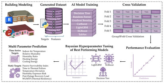
Figure 1. Overview of the utilized AI algorithms workflow for predicting building thermal resilience performance under power outages.

3.1. Dataset Structure

The dataset was created using an automated EnergyPlus workflow built with Python version 3.12.7 and EnergyPlus version 24.2.0, intended to assess the performance of residential buildings during prolonged summer power outages. As illustrated in Figure 2, four representative U.S. housing typologies, including detached, semi-detached, attached, and mid-rise apartment buildings, were developed as parametric BIM models in Autodesk Revit 2025. These BIM models provided standardized geometric and semantic definitions of walls, roofs, floors, and windows, which then served as the foundation for generating EnergyPlus-ready building energy models. The models were exported through the Green Building XML interface and imported into EnergyPlus, where the envelope constructions, materials and thermal characteristics defined in BIM (e.g., insulation layers, glazing systems, roof assemblies) remained fully traceable. This process created a direct link between BIM-defined building components, and the building energy models (BIM-to-BEM strategy). It also allows resilience predictions to be interpreted in terms of actual building components. The selected typologies were simulated across fourteen cities, each corresponding to one American Society of Heating, Refrigerating and Air-Conditioning Engineers (ASHRAE) climate zone, to cover a wide spectrum of envelope-to-volume ratios and climate conditions, both of which strongly influence passive thermal responses when power is lost.

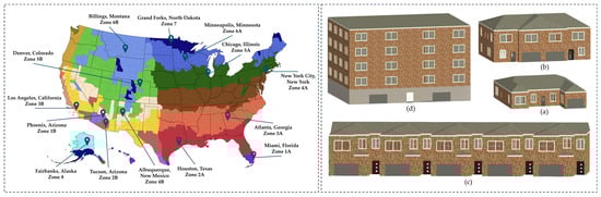
Figure 2. Selected U.S. locations representing ASHRAE climate zones 1–8 (left); and BIM models of four representative residential building typologies developed in Revit (right): (a) Detached, (b) Semi-detached, (c) Attached, and (d) Mid-rise apartment.

The selected cities were Miami, Florida (Zone 1A), Phoenix, Arizona (Zone 1B), Houston, Texas (Zone 2A), Tucson, Arizona (Zone 2B), Atlanta, Georgia (Zone 3A), Los Angeles, California (Zone 3B), New York City, New York (Zone 4A), Albuquerque, New Mexico (Zone 4B), Chicago, Illinois (Zone 5A), Denver, Colorado (Zone 5B), Minneapolis, Minnesota (Zone 6A), Billings, Montana (Zone 6B), Grand Forks, North Dakota (Zone 7), and Fairbanks, Alaska (Zone 8).

For each typology–climate combination, multiple envelope configurations were generated automatically by varying wall, roof, floor, and window assemblies selected from a predefined list of timber constructions, within IECC24 compliant performance ranges. The timber-based assemblies followed common structural dimensions, including 2 × 4 wood-framed walls, 2 × 8 rafters for roofs, and 2 × 10 joists for floors. In total, 70 unique wall types, 49 roof types, 17 floor types, and 30 window types were included. The walls, roofs, and floors incorporated a diverse set of insulation materials including expanded polystyrene, extruded polystyrene, PCM, aerogel panels, vacuum insulated panels, phenolic foam boards, mineral wool, fiberglass batt, cotton roll, cellulose loose-fill, cork insulation roll, green wall systems, and elastomeric reflective coatings. The thermal resistance (R-values) ranged from 2.27 to 16.79 m²·K/W for walls, 5.58 to 18.23 m²·K/W for roofs, and 7.58 to 13.14 m²·K/W for floors. Window configurations achieved thermal transmittance (U-values) ranging from 2.84 to 1.44 W/m²·K. The window set included single-pane, double-pane, and triple-pane glazing systems, with treatments such as low-emissivity (low-E) coatings, reflective layers, and specialized tints (blue-green, gray, green). A stratified sampling strategy was applied to efficiently explore this design space without requiring exhaustive simulation of all possible combinations.

Weather inputs were derived from TMY files constructed from hourly records spanning 2009–2023. For each climate, the hottest day of the year was identified and aligned with the middle of a standardized five-day simulation, which included one day of preconditioning, three full days of outage, and one recovery day, to represent the most extreme conditions for each climate.

The simulations were substantial yet manageable due to automation. Detached and semi-detached houses each had 501 scenarios per climate zone (500 retrofits plus one baseline), with runtimes of 5 and 7 s per simulation, respectively. Attached houses and apartment buildings each had 101 scenarios per climate zone (100 retrofits plus one baseline), with runtimes of 23 and 34 s per simulation. Considering all four building types across 14 climate zones, the workflow produced a total of 16,856 simulations, completed in 45.8 h of runtime.

Each simulation was run at a 3-min timestep and yielded 2400 data rows per scenario. Altogether, this produced a dataset of 40,454,400 rows of time-stamped indoor and outdoor conditions. The high temporal resolution enabled detailed monitoring of indoor air temperature, humidity, and heating and cooling loads, to capture both the degradation of conditions during outages and the recovery once power was restored. From these raw outputs, a suite of thermal resilience metrics was calculated, including PSI, Time to Thermal Failure (TTF), Temperature Deviation (TD), Humidity Exposure Risk (HER), Recovery Time, Post-Outage Recovery Load (PORL), and WUMTP.

The resulting dataset combines static and time-series features (inputs), and static and time-series targets (outputs) for AI model training. Static features include climate zone, building type, and envelope configuration, together with the baseline WUMTP value. Time-series features capture temporal and weather-related drivers such as simulation day and hour, power outage status, outdoor temperature, humidity, solar radiation, and wind speed. The prediction targets consist of both dynamic outputs (indoor temperature, relative humidity, humidity ratio, heating and cooling energy) and static resilience metrics. Table 2 summarizes all features and targets.

Table 2. Summary of dataset features and targets used for AI algorithms training.

Category	Variable Type	Variables
Static Features	Scenario-specific	Climate zone, Building type, Wall type, Roof type, Floor type, Window type, Baseline WUMTP
Time-series Features	Temporal and weather-related	Time index, Simulation day, Simulation hour, Power outage status, Outdoor dry-bulb temperature, Outdoor dewpoint temperature, Outdoor wet-bulb temperature, Humidity ratio, Relative humidity, Barometric pressure, Wind speed, Diffuse solar radiation, Direct solar radiation
Time-series Targets	Indoor Environmental outputs	Indoor air temperature, Relative humidity, Humidity ratio, Heating energy, Cooling energy
Static Targets	Thermal resilience metrics	PSI, TTF, TD, HER, Recovery Time, PORL, WUMTP

3.2. Data Preparation

Data preprocessing was performed to prepare the raw simulation outputs for AI model training. The dataset contained numerical and categorical features as well as multiple target variables. Numerical features were standardized using z-score scaling, a method that transforms each feature by subtracting its mean and dividing by its standard deviation. This results in a distribution with a mean of zero and a standard deviation of one, which effectively places all features on the same scale [47]. Scaling is important for features such as barometric pressure, which can have much larger ranges than other variables. By applying z-score scaling, all numerical inputs were normalized to prevent any single variable from disproportionately influencing the learning process.

Categorical features, which represented discrete scenario properties such as wall type or climate, were first cast to the category data type and then encoded using ordinal encoding. Ordinal encoding replaces each category with a unique integer label [48]. While these integers do not imply any numerical relationship between the categories, tree-based models can still split on these values effectively.

To have an unbiased evaluation, the dataset was divided into training and testing subsets using unique scenario IDs. 80% of scenario IDs were used for training, and the remaining 20% were reserved for testing. This prevented timesteps from the same scenario appearing in both sets, and eliminated data leakage and ensured appropriate model evaluation.

To further improve the reliability of model performance estimates, GroupKFold cross-validation was applied using scenario IDs as grouping variables. Cross-validation is a resampling technique used to assess how well a model generalizes to unseen data. In this method, the data is split into multiple “folds” or partitions. For each round, one fold is set aside for validation while the model is trained on the remaining folds. This is repeated K times, and the results are averaged to provide a stable estimate of performance [49]. In GroupKFold, all timesteps from the same scenario are kept together in the same fold to avoid data leakage. In this study, five folds were used, and performance metrics such as R² were averaged across all folds to reflect robust and realistic accuracy.

3.3. Model Selection

AI algorithms for building energy applications may include a variety of algorithms and methods, from classical regression and tree-based learners to DL architectures. In this study, DL refers specifically to deep learning models, ML refers to other machine learning models excluding DL, and AI encompasses both categories.

The dataset developed for this study is a large-scale hybrid tabular dataset with more than 40 million rows. It integrates time-series features (e.g., outdoor temperature, humidity, solar radiation, wind speed, power outage state) with static categorical descriptors (e.g., building type, wall, roof, floor, window) and generates both dynamic outputs (indoor temperature, humidity, energy) and static resilience metrics (e.g., PSI, WUMTP). The hybrid and high-dimensional nature of the dataset necessitated the selection of models designed for tabular learning and capable of handling mixed feature types at scale.

Recent benchmarking studies have shown that tree ensemble MLs outperform conventional DLs when applied to tabular data, and deliver higher predictive accuracy, lower computational cost, and reduced sensitivity to hyperparameter tuning [50]. Conventional DLs, when applied directly to tabular datasets, are frequently over-parameterized and lack the inductive biases required to exploit feature heterogeneity, often leading to suboptimal learning and weaker generalization [51,52,53]. By contrast, ensemble tree models dominate in practice due to their computational efficiency, interpretability, and inductive bias toward hyperplane-like decision boundaries [54], a trend further reinforced by their strong performance in building energy prediction studies [26,33].

Based on this evidence, five ensemble learning ML models were selected: RF, Gradient Boosting Machine (GBM), Categorical Boosting (CatBoost), LightGBM, and XGBoost. A single Decision Tree was also included as a baseline to benchmark performance relative to more advanced ensemble methods. To complement these models, TabNet (Attentive Interpretable Tabular Learning) was also adopted, which is a purpose-built DL architecture introduced by Google [55] and specifically designed for tabular datasets.

Figure 3 shows a comparison of the ML models used in this study. (a) The Decision Tree is a simple predictive model that uses a hierarchical structure to split input data based on feature importance [56]. Although intuitive and computationally efficient, Decision Tree models are typically vulnerable to overfitting due to their inherent simplicity. To mitigate this limitation, (b) RF employs an ensemble approach by training multiple decision trees in parallel, each constructed on random subsets of the training data (bootstrapped samples) [57]. By averaging predictions across these diverse trees, RF significantly reduces variance, enhances generalization, and prevents overfitting. Advancing further, (c) GBM sequentially builds trees, each dedicated to correcting residual errors generated by preceding trees. Unlike RF’s parallel structure, GBM learns iteratively, and progressively refines its predictive accuracy through cumulative error correction [58]. More efficient gradient boosting models, including (d) CatBoost, (e) LightGBM, and (f) XGBoost, have refined this approach, and introduced innovations that address computational efficiency, scalability, and model accuracy. CatBoost enhances standard gradient boosting by integrating ordered target encoding to efficiently handle categorical features without explicit preprocessing, combined with ordered boosting that prevents prediction shift [59]. LightGBM advances further by introducing a leaf-wise growth strategy, which prioritizes splits that yield maximum loss reduction, and employs histogram-based feature binning for increased computational efficiency, which is especially suitable for large-scale datasets [60]. XGBoost is widely recognized for its exceptional performance, which combines gradient boosting with parallelized, histogram-based split finding, regularization techniques (L1 and L2 penalties), and sophisticated handling of missing values via learned default directions [61].

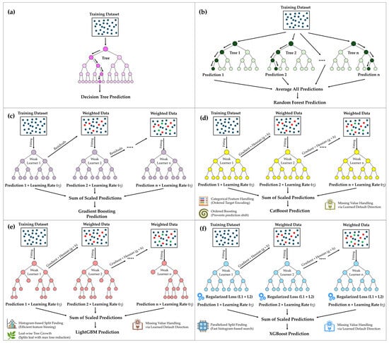
Figure 3. Visual comparison of six ML models used: (a) Decision Tree, (b) RF, (c) GBM, (d) CatBoost, (e) LightGBM, and (f) XGBoost.

3.4. Model Training

ML models were implemented within a multi-output regression framework using the MultiOutputRegressor class in scikit-learn in order to support simultaneous prediction of multiple targets. In this setup, a separate instance of the base learner (e.g., XGBoost, LightGBM, Decision Tree) was trained for each target, while the wrapper managed them as a unified pipeline. During training, the target matrix of shape (n_rows × 5) contained the time-series outputs including indoor temperature, relative humidity, humidity ratio, heating energy, and cooling energy, at each timestep. Each estimator learned to map the same hybrid feature set to its corresponding target, and at inference their predictions were concatenated row-wise to produce a five-dimensional output vector for every row. Static resilience indicators such as PSI, TTF, TD, HER, Recovery Time, PORL, and WUMTP were derived from the predicted time-series outputs by predicting the aggregated results at the scenario level using Scenario ID. This enabled the models to generate row-level short-term predictions of physical conditions at the timestep scale and also estimate scenario-level resilience metrics within a unified workflow.

Unlike conventional neural networks, TabNet processes input data through multiple sequential decision steps, and each consists of two specialized branches: an attention branch and a decision branch [55]. The attention branch utilizes an Attentive Transformer to dynamically learn masks over the initial input features, and to determine feature importance and select the most informative variables for each step. These selected features are then passed to the decision branch, where the Feature Transformer extracts relevant representations, splits the outputs into two components: one contributes to the final predictions through the aggregated features stream, while the other feeds forward to subsequent decision steps. This structured, stepwise feature selection and transformation process allows TabNet to explicitly model complex interactions and nonlinearities among static and time-varying inputs. Moreover, TabNet’s iterative masking mechanism enhances interpretability by highlighting feature contributions at each decision step, which makes it particularly powerful for handling high-dimensional hybrid datasets common in building energy prediction and thermal resilience assessments. As demonstrated in Figure 4, the input layer of TabNet received a total of 23 features, consisting of six categorical building descriptors (Climate, Building, Wall, Roof, Floor, Window) and 17 continuous numerical climate and simulation variables (e.g., outdoor temperature, humidity, solar radiation, wind speed). The output layer was defined as a linear regression head with five neurons, each corresponding to one of the direct time-series targets: indoor temperature, relative humidity, humidity ratio, heating energy, and cooling energy. In addition, seven scenario-level resilience metrics were computed in a post-processing step by aggregating and analyzing the predicted time-series outputs using Scenario ID.

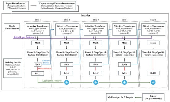
Figure 4. Architecture of the TabNet model used in this study.

All models were initially trained using their default hyperparameters to establish baseline performance for predicting the time-series targets. Hyperparameters represent model settings chosen before training, such as tree depth, number of estimators, or learning rate, which significantly influence a model’s predictive ability and efficiency [62]. After evaluating this baseline performance, the best-performing models underwent further optimization through Bayesian hyperparameter tuning using the Optuna framework. Bayesian optimization is an efficient search method that intelligently selects new hyperparameter configurations based on previous evaluation results, and quickly identifies optimal parameter combinations without exhaustively exploring the entire search space [63]. Specifically, Optuna sequentially proposed new hyperparameter sets informed by performance in earlier trials, aiming to maximize cross-validated R² scores [64]. During this optimization, the most influential hyperparameters tuned included the number of estimators (which determines how many trees or weak learners the model uses), maximum depth (controlling the complexity of each decision tree), and learning rate (governing the contribution of each new learner) across 20 iterative trials. Once the best hyperparameter values were identified, these optimized models were retrained on the full training dataset to enhance their predictive performance and generalizability. The optimized hyperparameters obtained through Bayesian tuning for the top performing ML models, including XGBoost, LightGBM, and Decision Tree, are summarized in Table 3.

Table 3. Optimized hyperparameters for the best-performing machine learning models.

Model	Hyperparameter	Optimized Value
XGBoost	Number of estimators	369
	Maximum depth	8
	Learning rate	0.2561
LightGBM	Number of estimators	495
	Maximum depth	8
	Learning rate	0.2032
Decision Tree	Maximum depth	19
	Minimum samples split	24
	Minimum samples per leaf	20
	Maximum features	0.6490

3.5. Model Evaluation

Model performance was evaluated using three complementary metrics: the coefficient of determination ($R^2$), normalized Mean Absolute Error (nMAE), and normalized Root Mean Squared Error (nRMSE). These metrics provide a comprehensive assessment of predictive accuracy and error magnitude relative to the scale of the observed values.

$R^2$ is a statistical metric that quantifies the proportion of variance in the observed data that is explained by the model’s predictions [65]. A higher $R^2$ value indicates that the model accounts for a larger share of the variability in the target variable and demonstrates a stronger correspondence between predicted and actual values, which consequently reflects a better overall model fit. The calculation of ${\mathrm{R}}^2$ expressed in Equation (1).

$${\mathrm{R}}^2=1-{\displaystyle \frac{\sum _{\mathrm{i}=1}^{\mathrm{n}}{({\mathrm{y}}_{\mathrm{i}}-{\widehat{\mathrm{y}}}_{\mathrm{i}})}^2}{\sum _{\mathrm{i}=1}^{\mathrm{n}}{({\mathrm{y}}_{\mathrm{i}}-\overline{\mathrm{y}})}^2}}$$

(1)

where ${\mathrm{y}}_{\mathrm{i}}$ is the observed value, ${\widehat{\mathrm{y}}}_{\mathrm{i}}$ is the predicted value, $\overline{\mathrm{y}}$ is the mean of the observed values, and $\mathrm{n}$ is the number of observations.

nMAE quantifies the average absolute difference between predicted and observed values, expressed as a percentage of the mean absolute value of the observations. It provides an interpretable measure of the typical prediction error relative to the scale of the target variable [66]. The calculation of nMAE is shown in Equation (2).

$$\mathrm{n}\mathrm{M}\mathrm{A}\mathrm{E}={\displaystyle \frac{\frac{1}{\mathrm{n}}\sum _{\mathrm{i}=1}^{\mathrm{n}}\left|{\mathrm{y}}_{\mathrm{i}}-\right.\left.{\widehat{\mathrm{y}}}_{\mathrm{i}}\right|}{\frac{1}{\mathrm{n}}\sum _{\mathrm{i}=1}^{\mathrm{n}}\left|{\mathrm{y}}_{\mathrm{i}}\right|}}\times 100$$

(2)

nRMSE quantifies the square root of the mean of squared differences between predicted and observed values, also expressed as a percentage of the mean absolute value of the observations. Because the errors are squared before averaging, nRMSE places greater emphasis on larger deviations, providing insight into both the magnitude and variability of prediction errors. The calculation of nRMSE is shown in Equation (3).

$$\mathrm{n}\mathrm{R}\mathrm{M}\mathrm{S}\mathrm{E}={\displaystyle \frac{\sqrt{\frac{1}{\mathrm{n}}\sum _{\mathrm{i}=1}^{\mathrm{n}}{({\mathrm{y}}_{\mathrm{i}}-{\widehat{\mathrm{y}}}_{\mathrm{i}})}^2}}{\frac{1}{\mathrm{n}}\sum _{\mathrm{i}=1}^{\mathrm{n}}\left|{\mathrm{y}}_{\mathrm{i}}\right|}}\times 100$$

(3)

A lower nMAE and nRMSE value indicates smaller errors relative to the scale of the target variable and reflects higher prediction accuracy and reduced deviation between predicted and observed values, which ultimately leads to a better model performance.

These metrics were computed for each time-series target, including indoor air temperature, relative humidity, humidity ratio, heating energy, and cooling energy. Normalizing MAE and RMSE as percentages allowed the error values to be expressed relative to the scale of each target variable. Using percentage-based metrics made the results more interpretable and enabled direct comparison of model performance across variables with different magnitudes and units.

4. Results

This section assesses how well AI algorithms that were created to forecast indoor environmental conditions during simulated power outage events perform. The results include time-series variables, along with static thermal resilience metrics. All models were initially trained using default hyperparameters to establish baseline performance, and the top-performing models were subsequently optimized using Bayesian hyperparameter tuning with the Optuna framework.

4.1. Baseline Evaluation Using Default Hyperparameters

Table 4 presents the baseline performance of all evaluated models in predicting time-series indoor environmental variables under default hyperparameter settings. The models were assessed across four key outputs, using R², nMAE, and nRMSE as evaluation metrics. These outputs include indoor temperature (°C), relative humidity (%), humidity ratio, and cooling energy (kJ/m²), each representing a critical aspect of building thermal performance during passive outage periods. Heating energy consumption was excluded from the time-series prediction targets, as it was found to be negligible across all climate zones. Even in cold climates, cooling energy demand remained the dominant factor due to elevated indoor temperatures during outage periods.

Table 4. Baseline model performance across individual time-series targets.

Model	Indoor Temperature (°C)			Relative Humidity (%)			Humidity Ratio			Cooling Energy (KJ/m2)
	R2	nMAE	nRMSE	R2	nMAE	nRMSE	R2	nMAE	nRMSE	R2	nMAE	nRMSE
XGBoost	0.992	1.02%	1.67%	0.998	1.07%	1.67%	0.995	2.92%	4.71%	0.994	9.39%	36.85%
LightGBM	0.994	0.87%	1.40%	0.998	1.14%	1.76%	0.996	2.81%	4.22%	0.896	12.75%	148.18%
Decision Tree	0.979	1.57%	2.68%	0.997	1.34%	2.15%	0.987	4.37%	7.43%	0.990	14.32%	46.79%
CatBoost	0.973	1.87%	3.04%	0.994	1.91%	2.95%	0.984	5.28%	8.21%	0.868	21.77%	167.25%
TabNet	0.945	2.99%	4.33%	0.986	2.82%	4.36%	−0.07	51.23%	67.15%	0.283	43.36%	390.60%

Among the evaluated models, both RF and GBM failed to complete the baseline training process and were therefore excluded from the comparative analysis. The RF model consistently encountered out-of-memory errors during training, even after multiple attempts using configurations ranging from 100 trees to as few as 10 trees. Despite being executed on a high-performance system with 32 GB of RAM, the model failed to run successfully and highlights its substantial memory demands and limited suitability for the size and complexity of this dataset. In contrast, the GBM model was allowed to train uninterrupted for over 50 h but never reached completion. This extreme runtime is attributed to GBM’s inherently sequential tree construction process, where trees are built one after another, which significantly increases computational load on large-scale data. Due to these limitations, both models were excluded from further evaluation and optimization.

For indoor temperature prediction, all models demonstrated strong accuracy, with R² values exceeding 0.94. LightGBM delivered the best performance and achieved the highest R² of 0.994 and the lowest nMAE of 0.87%. XGBoost followed closely, while Decision Tree and CatBoost also maintained solid performance. TabNet, however, recorded the highest error (nMAE = 2.99%) and the lowest R² (0.945), which indicate comparatively weaker accuracy but still acceptable performance for this target.

For relative humidity prediction, all models performed exceptionally well, with R² values exceeding 0.98. LightGBM and XGBoost delivered the best results, both achieved an R² of 0.998 and maintained low error rates (nMAE = 1.14% and 1.07%, respectively). Decision Tree and CatBoost also showed strong performance, with R² values of 0.997 and 0.994. TabNet produced a slightly higher error (nMAE = 2.82%) and a marginally lower R² of 0.986, yet still demonstrated robust predictive accuracy for this variable.

For humidity ratio prediction, LightGBM followed by XGBoost achieved the highest accuracy, with R² values of 0.996 and 0.995, and low error rates (nMAE = 2.81% and 2.92%, respectively). However, these error levels were slightly higher compared to those observed in the previous two targets. Decision Tree and CatBoost also performed well, with R² values of 0.987 and 0.984, and nMAE values of 4.37% and 5.28%, respectively. TabNet, in contrast, failed to capture the underlying pattern, and yielded a negative R² and extremely high errors (nMAE = 51.23%, nRMSE = 67.15%), which was an indication of a breakdown in predictive capability for this variable.

Cooling energy prediction posed the greatest challenge among all time-series targets. XGBoost delivered the most accurate results, with an R² of 0.994 and relatively low error rates (nMAE = 9.39%, nRMSE = 36.85%) compared to other models, though these errors were still considerably higher than those observed for the other targets. Decision Tree followed with a slightly lower R² of 0.990 and higher errors (nMAE = 14.32%, nRMSE = 46.79%). LightGBM’s performance declined for this variable, and R² dropped to 0.896 and nRMSE rose to 148.18%, despite strong results in the other outputs. CatBoost showed similar limitations, with an R² of 0.868 and an nRMSE of 167.25%. TabNet recorded the lowest accuracy, with an R² of just 0.283 and an nRMSE of 390.60%, which confirm its unsuitability for energy prediction tasks in this context.

Table 5 summarizes the overall baseline performance of each model by averaging their results across all time-series targets. Among all models, XGBoost achieved the highest overall R² of 99.48%, with low average errors (nMAE = 3.60%, nRMSE = 11.23%) and a moderate training time of 1148 s. These results indicate strong predictive performance across all outputs. The Decision Tree model ranked second, with an overall R² of 98.83%. However, its error rates were slightly higher (nMAE = 5.40%, nRMSE = 14.76%) and training time was notably longer at 2960 s, which reflects increased computational cost without a proportional gain in accuracy. LightGBM delivered strong overall accuracy (R² = 97.10%, nMAE = 4.39%) and had the fastest training time (638 s) among all evaluated models. However, its overall nRMSE was relatively high (38.89%), primarily due to elevated errors in predicting cooling energy, which affected the aggregate RMSE despite solid performance in the other targets. CatBoost maintained acceptable predictive performance (R² = 95.48%), but its error rates (nMAE = 7.71%, nRMSE = 45.36%) and long training time (4480 s) reduced its efficiency and practical value in this context. Finally, TabNet showed the weakest overall performance (R² = 53.60%) with high errors (nMAE = 25.10%, nRMSE = 116.61%) and the longest training duration (12,491 s). Despite being a deep learning architecture, it failed to generalize well which indicates a poor fit to this tabular, mixed static-temporal problem at the chosen setup. In summary, XGBoost provides the best balance of accuracy and training efficiency, LightGBM offered the fastest training time, suitable for applications that prioritize runtime, and Decision Tree provides a strong performance as a single-tree baseline.

Table 5. Overall baseline model performance and training time.

Model	Overall R2	Overall nMAE	Overall nRMSE	Training Time (s)
XGBoost	99.48%	3.60%	11.23%	1148
Decision Tree	98.83%	5.40%	14.76%	2960
LightGBM	97.10%	4.39%	38.89%	638
CatBoost	95.48%	7.71%	45.36%	4480
TabNet	53.60%	25.10%	116.61%	12,491

4.2. Enhanced Prediction Accuracy Through Hyperparameter Optimization

Table 6 presents the performance of the three best-performing models after undergoing Bayesian hyperparameter tuning. The results demonstrate substantial improvements across all time-series targets compared to their baseline configurations. For indoor temperature, all three models exhibited near-perfect accuracy, with R² values exceeding 0.99. XGBoost achieved the best results overall, with the highest R² (0.9992) and the lowest nMAE (0.33%) and nRMSE (0.53%). LightGBM followed closely with R² = 0.9987 and comparably low error metrics. The Decision Tree model also improved significantly (R² = 0.9931) but still trailed the ensemble-based models in predictive accuracy. In predicting relative humidity, all models again reached R² values above 0.998. XGBoost slightly outperformed the others, with R² = 0.9998 and the lowest nRMSE of 0.59%. LightGBM and Decision Tree followed closely and demonstrated consistent reliability in predicting this target. For humidity ratio, all three models delivered excellent results, with XGBoost once more demonstrated superior performance (R² = 0.9995, nMAE = 0.90%, nRMSE = 1.45%). Both Decision Tree and LightGBM showed improvements over their baselines.

Table 6. Performance of optimized models on time-series targets.

Time Series Metrics	XGBoost			Decision Tree			LightGBM
	R2	nMAE	nRMSE	R2	nMAE	nRMSE	R2	nMAE	nRMSE
Indoor Temperature C	0.9992	0.33%	0.53%	0.9931	0.82%	1.49%	0.9987	0.43%	0.66%
Relative Humidity %	0.9998	0.39%	0.59%	0.9989	0.62%	1.17%	0.9993	0.60%	0.95%
Humidity Ratio	0.9995	0.90%	1.45%	0.9954	2.28%	4.29%	0.9990	1.37%	2.09%
Cooling Energy KJ/m2	0.9993	2.79%	12.50%	0.9936	5.73%	38.71%	0.9007	6.91%	144.98%
Overall Performance	0.9994	1.10%	3.77%	0.9953	2.36%	11.42%	0.9744	2.33%	37.17%

Cooling energy prediction, the most challenging target, saw significant improvements across all models. XGBoost achieved R² = 0.9993, with nMAE reduced to 2.79%. This represents a substantial gain compared to the baseline. The Decision Tree model also improved considerably (R² = 0.9936), although its nRMSE remained higher at 38.71%. LightGBM, while performed well for the other targets, recorded a notably lower R² of 0.9007 and a very high nRMSE of 144.98%, which still indicates persistent difficulty in generalizing time-series cooling energy consumption predictions.

Overall, XGBoost consistently outperformed both Decision Tree and LightGBM across all time-series evaluation metrics as demonstrated in Table 6, with an overall R² of 0.9994, nMAE of 1.10%, and nRMSE of 3.77%. These results confirm XGBoost as the most accurate and reliable model for predicting indoor environmental conditions under power outage scenarios of the developed dataset. Although such high R² values may suggest overfitting, all reported metrics are based solely on the independent test set (20% of scenarios). The models were evaluated on unseen data, which demonstrates that the results reflect genuine predictive accuracy rather than overfitting.

Figure 5 presents the temporal profiles of CPU usage (%) and RAM usage (GB) during training for the best-performing ML models: Decision Tree, LightGBM, and XGBoost. The experiments were conducted on a workstation equipped with an Intel Core Ultra 9 185H CPU and 32 GB RAM. This analysis complements predictive performance metrics by providing insights into the computational efficiency of each algorithm.

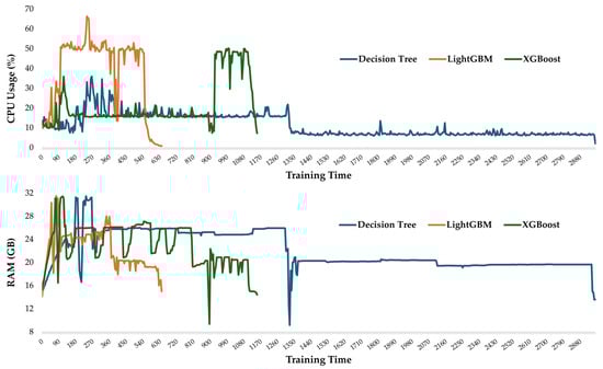
Figure 5. Temporal resource utilization during model training. Top: CPU usage (%) for Decision Tree, LightGBM, and XGBoost. Bottom: RAM usage (GB) for the same models.

RAM usage was broadly similar across the models, with Decision Tree consuming on average 22.05 GB (maximum 31.47 GB), LightGBM consuming 22.34 GB on average (maximum 31.5 GB), and XGBoost consuming 22.91 GB on average (maximum 31.44 GB). These results indicate that memory requirements were largely stable and not a differentiating factor between algorithms, although all models approached the system’s maximum available RAM of 32 GB at certain points due to the large scale of the dataset.

CPU utilization patterns, however, differed more substantially. Decision Tree was the most computationally efficient, with an average of 11.2% CPU usage and a peak of 36%. XGBoost required greater processing, 21.2% CPU usage on average and a peak of 50.1%. LightGBM was the most computationally expensive, averaging 37.7% CPU usage, approximately 1.78 times higher than XGBoost, with a peak of 66.3%. Despite these differences, none of the models approached full CPU capacity, which indicates that the training bottleneck was more memory-bound than processor-limited.

From a deployment perspective, maintenance cost refers to the effort required to update models when new data becomes available. Ensemble methods such as XGBoost are particularly advantageous in this regard, since they retrain quickly, require limited hyperparameter tuning, and maintain stable accuracy across updates. These properties make them well suited for operational environments where regular updates are necessary, such as thermal resilience analysis during power outages, where new climate data, buildings, or outage scenarios must be integrated rapidly and timely decision-making is critical. As highlighted by Shwartz-Ziv and Armon [50], DL is not always the preferred option for tabular data, and in contexts such as this study, ensemble methods demonstrate a more balanced trade-off between predictive accuracy, computational efficiency, and maintenance overhead.

Table 7 summarizes the predictive performance of XGBoost on seven key static thermal resilience indicators. The model achieved strong accuracy across all metrics, mainly in WUMTP (R² = 0.9521, nMAE = 5.98%) and PSI (R² = 0.9375, nMAE = 8.00%). Performance was also strong for TTF (R² = 0.8990) and PORL (R² = 0.7780). Moderate performance was observed in TD (R² = 0.7054) and HER (R² = 0.7054), while Recovery Time was the most difficult to predict (R² = 0.6618, nMAE = 17.80%), possibly due to its dependency on multi-phase thermal dynamics. These results show XGBoost’s capacity not only to predict dynamic environmental conditions but also to estimate key static resilience metrics with high accuracy.

Table 7. XGBoost prediction accuracy on static thermal resilience metrics.

Static Resiliency Metrics	R2	nMAE
Passive Survivability Index	0.9375	8.00%
Time to Thermal Failure	0.8990	7.35%
Temperature Deviation	0.7054	5.33%
Humidity Exposure Risk	0.7054	2.83%
Recovery Time	0.6618	17.80%
Post-Outage Recovery Load	0.7780	10.24%
WUMTP	0.9521	5.98%

Figure 6 uses residual scatter plots to give a more thorough visual examination of the model’s prediction behavior. These plots display the percentage error between predicted and actual values for each target variable across the test set. A horizontal dashed line at zero indicates perfect prediction.

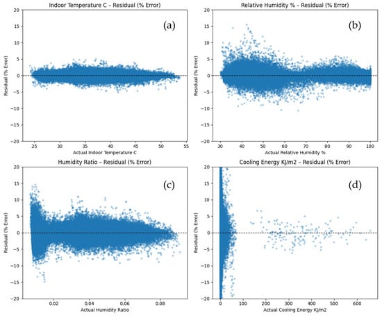
Figure 6. Residual scatter plots showing percent-error between predicted and actual values for (a) Indoor Temperature, (b) Relative Humidity, (c) Humidity Ratio, and (d) Cooling Energy.

As observed earlier in the performance metrics, the residuals for Indoor Temperature are tightly clustered around the zero-error line, with most deviations confined within ±2%, which indicates consistently strong predictive accuracy.

Relative Humidity follows a similar trend, although slightly more scattered in the 30% to 60% range, where residuals often cluster around +5% and occasionally rise up to +15%. This reflects minor overestimation by the model in moderately humid conditions but still within an acceptable margin.

For Humidity Ratio, the residuals appear more dispersed, especially at lower values between 0.00 and 0.02, where the majority of errors approach +10% and, in some cases, extend to +15%. However, for the rest of the range, the model maintains high accuracy, with most errors capped within ±5%, which confirms robust performance across varying humidity levels.

Cooling Energy predictions, on the other hand, exhibit a wider residual spread, especially close to zero actual values where overestimation becomes more noticeable. This behavior is likely attributed to periods of power outage where energy consumption is minimal, but the model continues to anticipate baseline cooling demand. However, as the actual cooling load rises, residuals converge closer to zero, suggesting that accuracy is enhanced during active thermal regulation.

4.3. Feature Relationship and Importance Analysis

The Pearson correlation heatmap presented in Figure 7 provides a visual overview of linear relationships among all input features. Several strong correlations are evident among environmental variables and form distinct dark regions on the map. For instance, Outdoor Air Drybulb Temperature, Dewpoint Temperature, Wetbulb Temperature, Relative Humidity, and Barometric Pressure form a tightly interrelated cluster, which is expected given their mutual dependence on climatic conditions. Likewise, Site Diffuse and Direct Solar Radiation appear as another correlated pair, which reflects shared solar exposure patterns.

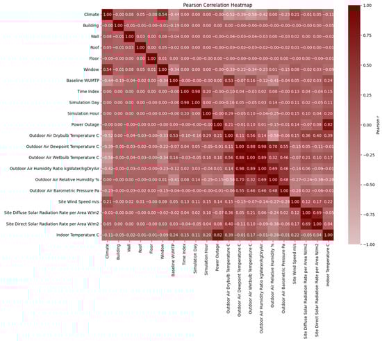
Figure 7. Pearson correlation heatmap showing the features’ linear relationships.

A second cluster is observed among simulation control variables such as Time Index, Simulation Day, and Simulation Hour, which show high correlation due to the sequential nature of time-series simulation data. These clusters confirm the internal consistency of the dataset and demonstrate that many environmental and temporal inputs are inherently dependent. In contrast, building envelope features do not exhibit any clear linear correlation with either environmental variables or with one another. This absence of linear relationships suggests that their influence on indoor thermal conditions may follow more complex or non-linear patterns, especially during power outage conditions. Since the objective of this study is to evaluate the role of building envelopes in enhancing passive thermal resilience, a model-based feature importance analysis is more appropriate than correlation analysis alone.

Figure 8 presents the ranked feature importances derived from the XGBoost model and highlights the contribution of each input feature to the prediction of all time-series targets, including indoor temperature, relative humidity, humidity ratio, and cooling energy, under simulated power outages. As expected, Power Outage dominates the feature space, and accounts for the largest share of importance, followed by Time Index, Baseline WUMTP, and other climate-related or time series parameters. While these features are highly influential, they represent fixed boundary conditions or scenario-defining parameters and therefore are not the focus of the evaluation in this study. To isolate the impact of design-modifiable parameters, a focused inset within Figure 8 presents the relative importance of the building envelopes, averaged across all targets and normalized to a 100% scale. Among these, Window holds the highest relative importance at 74.3%, followed by Floor (20.2%), Wall (4.2%), and Roof (1.4%). This distribution highlights that, during the hottest simulated week of the year under power outage conditions, windows exert the greatest influence on indoor temperature. This result likely stems from their exposure to direct and diffuse solar radiation, limited thermal resistance, and central role in heat gain, making them a key driver of passive thermal behavior across multiple indoor conditions.

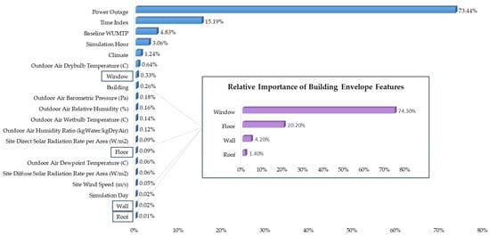
Figure 8. Feature importance ranking derived from the XGBoost model across all input variables, with a focus box illustrating the relative contribution of building envelope components.

5. Discussion

The present paper offers four contributions to the field of the study. First, this study advances the field by expanding the range of resilience metrics applied. Prior works have typically relied on a limited set of resilience metrics which are primarily temperature-based metrics. In contrast, this study employed not only temperature-related aspects but also humidity exposure that can lead to mold growth and indoor air quality risks, the duration of recovery after outages, and the additional cooling energy required for buildings to return to normal operation. Second, this paper provides a methodological contribution by extending AI algorithms beyond normal operating conditions to predict building resilience during power outages. Unlike earlier studies that focused solely on standard operational scenarios, this study fills that gap by developing a Fine-tuned XGBoost model capable of accurate predictions with R² of 0.9994 for time-series indoor conditions, and R² of 0.81 for static resilience metrics. This model is trained on 16,856 EnergyPlus-derived 5-day simulation period with 72 h of power outage (about 40 million rows of data) with 45.8 h needed to generate the simulation dataset and trained 1148 s. Third, a systematic evaluation of tree-based, ensemble boosting, and deep learning models revealed that ensemble boosting algorithms consistently outperformed both single-tree and deep learning approaches, with XGBoost delivering the highest predictive accuracy and LightGBM demonstrating the fastest training time (638 s). Finally, feature importance analysis identified windows as the dominant contributor (74.3%) to envelope-related performance, emphasizing their pivotal role in indoor thermal stability during blackouts compared to other components such as walls, roofs, and floors.

The study also has limitations. First, EnergyPlus simulations were the only source of the dataset. Although systematic, these simulations are unable to accurately represent real-world uncertainties like equipment use or occupant behavior. Field data should be used in future research to verify and improve the models. Second, the analysis focused only on four residential archetypes. Complex and larger structures, like mixed-use or high-rise buildings, were excluded. To increase generalizability, the dataset should be expanded to include a greater variety of building types. Third, the framework addressed only summer outages and envelope-driven performance. Other scenarios, such as winter outages, HVAC recovery strategies, and integration of renewable energy or storage systems, were not considered. Expanding to these dimensions would provide a more comprehensive view of resilience. Lastly, even though ensemble-based AI models were very accurate, it was more difficult to predict certain goals like cooling energy and recovery time. Future work could explore hybrid approaches that combine AI with simplified physics models to improve reliability.

6. Conclusions

Seven AI algorithms were evaluated, including Decision Tree, RF, GBM, CatBoost, LightGBM, XGBoost, and TabNet, to predict both time-series indoor conditions (temperature, relative humidity, humidity ratio, cooling and heating demand) and static resilience metrics (PSI, TTF, TD, HER, Recovery Time, PORL, WUMTP). XGBoost demonstrated the best performance. Predictions of temperature and relative humidity exceeded R² = 0.999, while humidity ratio and cooling energy achieved R² values of 0.995 and 0.994, respectively. Resilience metrics were also predicted effectively: WUMTP (R² = 0.95), PSI (R² = 0.94), and TTF (R² = 0.90). The comparison across algorithms showed that ensemble boosting methods outperformed both DL and single-tree models. While TabNet showed weaker predictions (R² = 0.54 overall), ensemble models proved more efficient for hybrid datasets that com-bine time series and static inputs and outputs.

The study shows that AI can reduce computational demand dramatically. The training dataset was generated through 45.8 h of automated EnergyPlus simulations, yet the AI models trained on this dataset required only 638 s for LightGBM and 1148 s for XGBoost. Once trained, they deliver predictions in seconds and eliminate the need for repeated large-scale simulations for each new case.

The impact of envelope components was measured using feature importance analysis, and windows accounted for 74.3% of the envelope-related impact, compared to 20.2% for floors, 4.2% for walls, and 1.4% for roofs. This supports the prioritization of techniques like advanced glazing, shading, and films and emphasizes glazing as the primary factor in passive survivability during blackouts in hot seasons.

References

- Schulz, N. Lessons from the London Climate Change Strategy: Focusing on Combined Heat and Power and Distributed Generation. J. Urban Technol. 2010, 17, 3–23. [Google Scholar] [CrossRef]
- Keirstead, J.; Jennings, M.; Sivakumar, A. A review of urban energy system models: Approaches, challenges and opportunities. Renew. Sustain. Energy Rev. 2012, 16, 3847–3866. [Google Scholar] [CrossRef]
- Rehman, H.u.; Nik, V.M.; Ramesh, R.; Ala-Juusela, M. Quantifying and Rating the Energy Resilience Performance of Buildings Integrated with Renewables in the Nordics under Typical and Extreme Climatic Conditions. Buildings 2024, 14, 2821. [Google Scholar] [CrossRef]
- Chen, Y.; Moufouma-Okia, W.; Masson-Delmotte, V.; Zhai, P.; Pirani, A. Recent Progress and Emerging Topics on Weather and Climate Extremes Since the Fifth Assessment Report of the Intergovernmental Panel on Climate Change. Annu. Rev. Environ. Resour. 2018, 43, 35–59. [Google Scholar] [CrossRef]
- Steinhaeuser, K.; Ganguly, A.R.; Chawla, N.V. Multivariate and multiscale dependence in the global climate system revealed through complex networks. Clim. Dyn. 2012, 39, 889–895. [Google Scholar] [CrossRef]
- Ciscar, J.-C.; Dowling, P. Integrated assessment of climate impacts and adaptation in the energy sector. Energy Econ. 2014, 46, 531–538. [Google Scholar] [CrossRef]
- Auffhammer, M.; Mansur, E.T. Measuring climatic impacts on energy consumption: A review of the empirical literature. Energy Econ. 2014, 46, 522–530. [Google Scholar] [CrossRef]
- Hatvani-Kovacs, G.; Belusko, M.; Skinner, N.; Pockett, J.; Boland, J. Heat stress risk and resilience in the urban environment. Sustain. Cities Soc. 2016, 26, 278–288. [Google Scholar] [CrossRef]
- Hatvani-Kovacs, G.; Belusko, M.; Skinner, N.; Pockett, J.; Boland, J. Drivers and barriers to heat stress resilience. Sci. Total Environ. 2016, 571, 603–614. [Google Scholar] [CrossRef]
- Keramitsoglou, I.; Sismanidis, P.; Analitis, A.; Butler, T.; Founda, D.; Giannakopoulos, C.; Giannatou, E.; Karali, A.; Katsouyanni, K.; Kendrovski, V.; et al. Urban thermal risk reduction: Developing and implementing spatially explicit services for resilient cities. Sustain. Cities Soc. 2017, 34, 56–68. [Google Scholar] [CrossRef]
- Rafael, S.; Martins, H.; Sá, E.; Carvalho, D.; Borrego, C.; Lopes, M. Influence of urban resilience measures in the magnitude and behaviour of energy fluxes in the city of Porto (Portugal) under a climate change scenario. Sci. Total Environ. 2016, 566–567, 1500–1510. [Google Scholar] [CrossRef]
- Mola, M.; Feofilovs, M.; Romagnoli, F. Energy resilience: Research trends at urban, municipal and country levels. Energy Procedia 2018, 147, 104–113. [Google Scholar] [CrossRef]
- U.S. Green Building Council. Resilient by Design: USGBC Offers Sustainability Tools for Enhanced Resilience; U.S. Green Building Council: Washington, DC, USA, 2018. [Google Scholar]
- Sun, K.; Zhang, W.; Zeng, Z.; Levinson, R.; Wei, M.; Hong, T. Passive cooling designs to improve heat resilience of homes in underserved and vulnerable communities. Energy Build. 2021, 252, 111383. [Google Scholar] [CrossRef]
- Hong, T.; Malik, J.; Krelling, A.; O’Brien, W.; Sun, K.; Lamberts, R.; Wei, M. Ten questions concerning thermal resilience of buildings and occupants for climate adaptation. Build. Environ. 2023, 244, 110806. [Google Scholar] [CrossRef]
- Ozarisoy, B. Energy effectiveness of passive cooling design strategies to reduce the impact of long-term heatwaves on occupants’ thermal comfort in Europe: Climate change and mitigation. J. Clean. Prod. 2022, 330, 129675. [Google Scholar] [CrossRef]
- Attia, S.; Levinson, R.; Ndongo, E.; Holzer, P.; Berk Kazanci, O.; Homaei, S.; Zhang, C.; Olesen, B.W.; Qi, D.; Hamdy, M.; et al. Resilient cooling of buildings to protect against heat waves and power outages: Key concepts and definition. Energy Build. 2021, 239, 110869. [Google Scholar] [CrossRef]
- Sailor, D.J.; Baniassadi, A.; O’Lenick, C.R.; Wilhelmi, O.V. The growing threat of heat disasters. Environ. Res. Lett. 2019, 14, 054006. [Google Scholar] [CrossRef]
- Rahmani, S.; Kaoula, D.; Hamdy, M. Exploring the thermal behaviour of building materials: Terracotta, concrete hollow block and hollow brick, under the arid climate, case study of Biskra-Algeria. Mater. Today Proc. 2022, 58, 1380–1388. [Google Scholar] [CrossRef]
- Mirzabeigi, S.; Razkenari, M. Multiple benefits through residential building energy retrofit and thermal resilient design. In Proceedings of the 6th Residential Building Design & Construction Conference, University Park, PA, USA, 11–12 May 2022. [Google Scholar]
- Sepasgozar, S.; Karimi, R.; Farahzadi, L.; Moezzi, F.; Shirowzhan, S.M.; Ebrahimzadeh, S.; Hui, F.; Aye, L. A Systematic Content Review of Artificial Intelligence and the Internet of Things Applications in Smart Home. Appl. Sci. 2020, 10, 3074. [Google Scholar] [CrossRef]
- Saleem, R.; Yuan, B.; Kurugollu, F.; Anjum, A.; Liu, L. Explaining deep neural networks: A survey on the global interpretation methods. Neurocomputing 2022, 513, 165–180. [Google Scholar] [CrossRef]
- Kondath, N.; Myat, A.; Soh, Y.L.; Tung, W.L.; Eugene, K.A.M.; An, H. Enhancing Day-Ahead Cooling Load Prediction in Tropical Commercial Buildings Using Advanced Deep Learning Models: A Case Study in Singapore. Buildings 2024, 14, 397. [Google Scholar] [CrossRef]
- Abdel-Jaber, F.; Dirks, K.N. A Review of Cooling and Heating Loads Predictions of Residential Buildings Using Data-Driven Techniques. Buildings 2024, 14, 752. [Google Scholar] [CrossRef]
- Gong, Y.; Zoltán, E.S.; Gyergyák, J. A Neural Network Trained by Multi-Tracker Optimization Algorithm Applied to Energy Performance Estimation of Residential Buildings. Buildings 2023, 13, 1167. [Google Scholar] [CrossRef]
- Mehraban, M.H.; Alnaser, A.A.; Sepasgozar, S.M.E. Building Information Modeling and AI Algorithms for Optimizing Energy Performance in Hot Climates: A Comparative Study of Riyadh and Dubai. Buildings 2024, 14, 2748. [Google Scholar] [CrossRef]
- Muslimsyah, M.; Safwan, S.; Novandri, A. Comprehensive Assessment of Indoor Thermal in Vernacular Building Using Machine Learning Model with GAN-Based Data Imputation: A Case of Aceh Region, Indonesia. Buildings 2025, 15, 2448. [Google Scholar] [CrossRef]
- Tahmasebinia, F.; Jiang, R.; Sepasgozar, S.; Wei, J.; Ding, Y.; Ma, H. Implementation of BIM Energy Analysis and Monte Carlo Simulation for Estimating Building Energy Performance Based on Regression Approach: A Case Study. Buildings 2022, 12, 449. [Google Scholar] [CrossRef]
- Qin, H.; Yu, Z.; Li, Z.; Li, H.; Zhang, Y. Nearly Zero-Energy Building Load Forecasts through the Competition of Four Machine Learning Techniques. Buildings 2024, 14, 147. [Google Scholar] [CrossRef]
- Abdel-Jaber, F.; Dirks, K.N. Thermal Load Prediction in Residential Buildings Using Interpretable Classification. Buildings 2024, 14, 1989. [Google Scholar] [CrossRef]
- Aparicio-Ruiz, P.; Barbadilla-Martín, E.; Guadix, J.; Nevado, J. Analysis of Variables Affecting Indoor Thermal Comfort in Mediterranean Climates Using Machine Learning. Buildings 2023, 13, 2215. [Google Scholar] [CrossRef]
- Liu, H.; Ma, E. An Explainable Evaluation Model for Building Thermal Comfort in China. Buildings 2023, 13, 3107. [Google Scholar] [CrossRef]
- Mehraban, M.H.; Sepasgozar, S.M.E.; Ghomimoghadam, A.; Zafari, B. AI-enhanced automation of building energy optimization using a hybrid stacked model and genetic algorithms: Experiments with seven machine learning techniques and a deep neural network. Results Eng. 2025, 26, 104994. [Google Scholar] [CrossRef]
- Norouzi, P.; Maalej, S.; Mora, R. Applicability of Deep Learning Algorithms for Predicting Indoor Temperatures: Towards the Development of Digital Twin HVAC Systems. Buildings 2023, 13, 1542. [Google Scholar] [CrossRef]
- Iqbal, F.; Mirzabeigi, S. Digital Twin-Enabled Building Information Modeling–Internet of Things (BIM-IoT) Framework for Optimizing Indoor Thermal Comfort Using Machine Learning. Buildings 2025, 15, 1584. [Google Scholar] [CrossRef]
- Akander, J.; Bakhtiari, H.; Ghadirzadeh, A.; Mattsson, M.; Hayati, A. Development of an AI Model Utilizing Buildings’ Thermal Mass to Optimize Heating Energy and Indoor Temperature in a Historical Building Located in a Cold Climate. Buildings 2024, 14, 1985. [Google Scholar] [CrossRef]
- Telicko, J.; Krumins, A.; Nikitenko, A. Development and Evaluation of Neural Network Architectures for Model Predictive Control of Building Thermal Systems. Buildings 2025, 15, 2702. [Google Scholar] [CrossRef]
- Krelling, A.F.; Lamberts, R.; Malik, J.; Hong, T. A simulation framework for assessing thermally resilient buildings and communities. Build. Environ. 2023, 245, 110887. [Google Scholar] [CrossRef]
- Wang, Y.; Yue, Q.; Lu, X.; Gu, D.; Xu, Z.; Tian, Y.; Zhang, S. Digital twin approach for enhancing urban resilience: A cycle between virtual space and the real world. Resilient Cities Struct. 2024, 3, 34–45. [Google Scholar] [CrossRef]
- Zhang, L.; Wen, J.; Li, Y.; Chen, J.; Ye, Y.; Fu, Y.; Livingood, W. A review of machine learning in building load prediction. Appl. Energy 2021, 285, 116452. [Google Scholar] [CrossRef]
- Li, H.; Hong, T. A digital twin platform for building performance monitoring and optimization: Performance simulation and case studies. Build. Simul. 2025, 18, 1561–1579. [Google Scholar] [CrossRef]
- Tao, M.; Gou, Z.; Ma, N. Assessment of thermal comfort and thermal resilience in dwellings during heat waves: A case study of a near-zero energy house. J. Build. Eng. 2025, 109, 113052. [Google Scholar] [CrossRef]
- Ismail, N.; Ouahrani, D.; Al Touma, A. Quantifying thermal resilience of office buildings during power outages: Development of a simplified model metric and validation through experimentation. J. Build. Eng. 2023, 72, 106564. [Google Scholar] [CrossRef]
- Sheng, M.; Reiner, M.; Sun, K.; Hong, T. Assessing thermal resilience of an assisted living facility during heat waves and cold snaps with power outages. Build. Environ. 2023, 230, 110001. [Google Scholar] [CrossRef]
- Homaei, S.; Hamdy, M. Thermal resilient buildings: How to be quantified? A novel benchmarking framework and labelling metric. Build. Environ. 2021, 201, 108022. [Google Scholar] [CrossRef]
- Mirzabeigi, S.; Homaei, S.; Razkenari, M.; Hamdy, M. The Impact of Building Retrofitting on Thermal Resilience Against Power Failure: A Case of Air-Conditioned House. In Proceedings of the 5th International Conference on Building Energy and Environment; Springer: Singapore, 2023; pp. 2609–2619. [Google Scholar]
- Izenman, A.J. Modern Multivariate Statistical Techniques; Springer: Berlin/Heidelberg, Germany, 2008; Volume 1, Available online: https://link.springer.com/book/10.1007/978-0-387-78189-1 (accessed on 30 October 2025).
- Pedregosa, F.; Varoquaux, G.; Gramfort, A.; Michel, V.; Thirion, B.; Grisel, O.; Blondel, M.; Prettenhofer, P.; Weiss, R.; Dubourg, V. Scikit-learn: Machine learning in Python. J. Mach. Learn. Res. 2011, 12, 2825–2830. [Google Scholar]
- Kohavi, R. A study of cross-validation and bootstrap for accuracy estimation and model selection. In Proceedings of the International Joint Conference on Artificial Intelligence (IJCAI), Montreal, QC, Canada, 20–25 August 1995; pp. 1137–1145. [Google Scholar]
- Shwartz-Ziv, R.; Armon, A. Tabular data: Deep learning is not all you need. Inf. Fusion 2022, 81, 84–90. [Google Scholar] [CrossRef]
- Goodfellow, I.; Bengio, Y.; Courville, A.; Bengio, Y. Deep Learning; MIT Press Cambridge: Cambridge, MA, USA, 2016; Volume 1. [Google Scholar]
- Shavitt, I.; Segal, E. Regularization learning networks: Deep learning for tabular datasets. Adv. Neural Inf. Process. Syst. 2018, 31. Available online: https://proceedings.neurips.cc/paper_files/paper/2018/hash/500e75a036dc2d7d2fec5da1b71d36cc-Abstract.html (accessed on 30 October 2025).
- Xu, L.; Skoularidou, M.; Cuesta-Infante, A.; Veeramachaneni, K. Modeling tabular data using conditional gan. Adv. Neural Inf. Process. Syst. 2019, 32. [Google Scholar]
- Lundberg, S.M.; Erion, G.G.; Lee, S.-I. Consistent individualized feature attribution for tree ensembles. arXiv 2018, arXiv:1802.03888. [Google Scholar]
- Arik, S.Ö.; Pfister, T. TabNet: Attentive Interpretable Tabular Learning. Proc. AAAI Conf. Artif. Intell. 2021, 35, 6679–6687. [Google Scholar] [CrossRef]
- Breiman, L.; Friedman, J.; Olshen, R.A.; Stone, C.J. Classification and Regression Trees; Chapman and Hall/CRC: Boca Raton, FL, USA, 2017. [Google Scholar] [CrossRef]
- Breiman, L. Random forests. Mach. Learn. 2001, 45, 5–32. [Google Scholar] [CrossRef]
- Friedman, J.H. Greedy function approximation: A gradient boosting machine. Ann. Stat. 2001, 29, 1189–1232. [Google Scholar] [CrossRef]
- Prokhorenkova, L.; Gusev, G.; Vorobev, A.; Dorogush, A.V.; Gulin, A. CatBoost: Unbiased boosting with categorical features. Adv. Neural Inf. Process. Syst. 2018, 31. [Google Scholar]
- Ke, G.; Meng, Q.; Finley, T.; Wang, T.; Chen, W.; Ma, W.; Ye, Q.; Liu, T.-Y. Lightgbm: A highly efficient gradient boosting decision tree. Adv. Neural Inf. Process. Syst. 2017, 30. [Google Scholar]
- Chen, T.; Guestrin, C. Xgboost: A scalable tree boosting system. In Proceedings of the 22nd ACM Sigkdd International Conference on Knowledge Discovery and Data Mining, San Francisco, CA, USA, 13–17 August 2016; pp. 785–794. [Google Scholar]
- Bischl, B.; Binder, M.; Lang, M.; Pielok, T.; Richter, J.; Coors, S.; Thomas, J.; Ullmann, T.; Becker, M.; Boulesteix, A.L. Hyperparameter optimization: Foundations, algorithms, best practices, and open challenges. Wiley Interdiscip. Rev. Data Min. Knowl. Discov. 2023, 13, e1484. [Google Scholar] [CrossRef]
- Snoek, J.; Larochelle, H.; Adams, R.P. Practical bayesian optimization of machine learning algorithms. Adv. Neural Inf. Process. Syst. 2012, 25. [Google Scholar]
- Akiba, T.; Sano, S.; Yanase, T.; Ohta, T.; Koyama, M. Optuna: A next-generation hyperparameter optimization framework. In Proceedings of the 25th ACM SIGKDD International Conference on Knowledge Discovery & Data Mining, Anchorage, AK, USA, 4–8 August 2019; pp. 2623–2631. [Google Scholar]
- Figueiredo Filho, D.B.; Júnior, J.A.S.; Rocha, E.C. What is R2 all about? Leviathan 2011, 60–68. [Google Scholar] [CrossRef]
- Roider, J.; Nguyen, A.; Zanca, D.; Eskofier, B.M. Assessing the Performance of Remaining Time Prediction Methods for Business Processes. IEEE Access 2024, 12, 130583–130601. [Google Scholar] [CrossRef]
Disclaimer/Publisher’s Note: The statements, opinions and data contained in all publications are solely those of the individual author(s) and contributor(s) and not of MDPI and/or the editor(s). MDPI and/or the editor(s) disclaim responsibility for any injury to people or property resulting from any ideas, methods, instructions or products referred to in the content. |
© 2025 by the authors. Licensee MDPI, Basel, Switzerland. This article is an open access article distributed under the terms and conditions of the Creative Commons Attribution (CC BY) license (https://creativecommons.org/licenses/by/4.0/).