Abstract
The effectiveness of mixing ventilation for contaminant removal and maintaining indoor air quality remains an active topic of debate. In shared multi-person spaces, it is common for occupants to experience uneven exposure levels due to variations in system configuration and seating arrangements. Previous studies have primarily considered static occupancy schemes, leaving a gap in understanding how dynamic patterns of use interact with ventilation design. This study investigates the combined effects of system settings and occupancy patterns on ventilation effectiveness (VE), while also exploring whether lower ventilation rates can still sustain acceptable air quality. Validated Computational Fluid Dynamics (CFD) models were developed to simulate multiple scenarios involving three ceiling heights, two inlet and exhaust configurations, and three occupancy patterns. Analysis of air quality at the breathing zone reveals that the spatial arrangement of ventilation inlets and exhausts substantially influences VE, with optimized layouts improved system effectiveness by approximately 20%. Seating arrangement was similarly important, with favorable positioning relative to inlets improving perceived air quality by up to 25%. In addition, modest increases in ceiling height reduced the ventilation rate needed to maintain equivalent air quality, suggesting opportunities for energy savings without compromising occupant health. Overall, this study demonstrates that the interaction between system configuration and occupancy has a stronger impact on ventilation performance. These findings underscore the importance of integrated design strategies that align ventilation layout with occupant distribution to achieve both efficiency and equity in indoor environments.
1. Introduction
According to ASHRAE, ventilation effectiveness (VE) is defined in terms of contaminant removal effectiveness, which measures the efficiency of a ventilation system in reducing the concentration of airborne pollutants []. The air distribution system has a crucial role in the performance of ventilation, contaminant removal, and indoor air quality []. For evaluating the performance of ventilation, an assessment index is defined to measure ventilation effectiveness across different areas within a room []. Ventilation efficiency can be assessed by calculating the ratio of the contaminant concentration at specific points, which is a quantitative measure of how effectively the ventilation system dilutes contaminants. The ventilation effectiveness of the system is directly influenced by the air distribution, which governs how contaminants (CO2) are transported and removed from the breathing zone [].
The Mixing Ventilation system (MV) has been the most popular and widely used air conditioning system for decades, and its efficiency has been a focus of numerous studies [,]. Many studies have focused on optimizing the MV system parameters to improve the effectiveness of removing contaminants and reducing infection threats [], such as increasing fresh air supply to dilute the concentration of contaminants to decrease the risk of cross infection [,]. Some previous studies suggested that higher air change rates guarantee the contaminant concentration reduction [,]. However, ventilation effectiveness is not solely dependent on the volume of air supplied (ventilation flow rate); it also hinges on how that air is distributed and interacts with the indoor environment []. For example, in the study by Van Hoof and Blocken (2020) on supply velocity in mixing ventilation systems, they found that employing a time-periodic supply reduces supply flow rates, resulting in about a 20% increase in contaminant removal effectiveness and reduced overall pollutant concentrations over time []. Although theoretically, increasing ventilation airflow rate does dilute concentrations when the contaminant source is constant, it may not increase the ventilation effectiveness, where ventilation system design is more important than the flow rate [].
Liu et al. (2022) found that although increasing the air change rate in the MV system has reduced the particle concentration, the improvement of the ventilation was not proportional to the ventilation rate []. Moreover, Wang et al. (2021) showed that a higher ventilation rate does not necessarily result in better indoor air quality (IAQ) if airflow patterns are not adequately designed []; more studies emerged and focused on the complex nature of the ventilation system, which needs proper evaluation at the design stage itself for robust indoor environmental quality.
The ventilation system layout can significantly influence air distribution and its effectiveness, affecting how contaminants are removed and how fresh air is circulated throughout the space []. Extensive research has shown that inlet and exhaust placement strongly affect indoor air quality and contaminant removal, with the location of exhaust vents being particularly critical. For example, Qin et al. (2023) showed that placing an exhaust on the same side as the supply diffuser in a classroom yielded the best results, lowering CO2 levels from 753 to 726 ppm [].
Studies have consistently shown that outlet placement with respect to height plays a critical role in indoor air distribution and contaminant removal. Placing outlets near particle landing areas, above occupants, or at different elevations has been found to improve removal efficiency, while combinations such as lower wall exhausts with swirl diffusers further enhance ventilation performance [,,,]. The importance of the diffusers’ location elevation on air distribution can be further emphasized in research focusing on ceiling levels. Wang and Hong (2023) showed that lower ceilings increase contaminant transmission [] (pp. 0–22), while Hunt and Linden (2005) developed a ventilation model incorporating the height, ventilation rate, and the buoyancy flux []. A number of studies on the occupant’s effect on air distribution have focused on cross-infection during COVID-19, [] (pp. 109–158), typically examining seating arrangements for as few as two occupants. Katramiz et al. (2021) studied the arrangement of occupants in MV + PV systems and found that a face-to-face arrangement, where both occupants were positioned laterally equidistant from the diffusers (X = 0.5 m), reduced contamination levels by 85% compared to the tandem arrangement []. In the study by Ai and Melikove (2018), they recommend that workstations should be arranged in a face-to-back orientation, and face-to-face orientation should be reduced, and the workers should be located side-to-side []. Decreasing the interaction between supplied air and exhaled flow intensifies the risk between close occupants and reduces system efficiency. Qin et al. (2023) examined a 50-person classroom and found that the optimal single-exhaust placement for reducing breathing contaminants depends on the room’s airflow pattern []. Moreover, Abuimara et al. (2021) examined the impact of occupants’ spatial distributions on office buildings’ energy and air quality performance []. They observed that changes in occupants’ distribution scenarios corresponded with an increase in the number of contaminant levels, which varied in magnitude, and thus, no orientation-related trends can be drawn from the results. The optimal ventilation system settings for varying occupant density and their positions and proximity to the inlet and exhaust vents remain unclear in a shared office with a mixing ventilation system. Therefore, this paper investigates the spread of human-exhaled contaminants across different occupancy levels, evaluating their interaction with key system settings (air change rates, ceiling heights, and exhaust locations (Section 3.1). The goal is to assess whether airflow rates can be reduced without compromising indoor air quality, thereby highlighting potential energy savings. It further explores why rearrangement of occupants and ventilation layouts is necessary to enhance breathing zone air quality and overall system performance (Section 3.2) and evaluates whether average ventilation effectiveness can serve as a reliable indicator for system performance (Section 3.3).
This study utilizes validated computational fluid dynamics (CFD) simulations to examine the effects of exhaust location and ceiling height on ventilation effectiveness and the removal of exhaled contaminants. To model airborne contamination, CO2 levels were employed as a representative breathing contaminant, as used in many previous studies [,,], to calculate ventilation effectiveness. A total of 17 models were simulated to evaluate indoor air quality at the breathing level, with the ventilation effectiveness (VE) of each configuration systematically analyzed. The novelty of this paper lies in studying a real-world shared office setting and evaluating its performance in various conditions, considering various occupancy patterns and arrangements to examine optimal VE.
2. Methods
2.1. Details of the Experimental Facility
A shared office room with dimensions of 14.02 m × 9.75 m × 2.9 m (L × W × H) located in Baton Rouge, LA, USA, was investigated. The office room was equipped with a mixing ventilation system (MV) containing five supply diffusers and two exhaust vents, located at 2.9 m (9.5 feet) above the floor. The squared inlet vents were 0.6 m × 0.6 m, and the exhaust vents were 0.6 m × 0.8 m, respectively. A pictorial representation of the room is shown in Figure 1a.
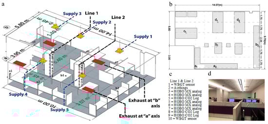
Figure 1.
Experimental room model. (a) An isometric view of the experimental facility. (b) The room plan with the location of the sensors. (c) Sensor locations guideline for vertical Line 1 and 2 in Figure 1a. (d) A picture of the experimental facility.
2.2. Developing the Computational Model
An experimental study was conducted to obtain the required boundary conditions for Computational Fluid Dynamics (CFD) simulations and to validate simulation results. Air was supplied to the room at a controlled flow rate, temperature, and humidity, measured using a TSI Alnor EBT731 (TSI Inc., Minneapolis, MN, USA) (https://tsi.com/products/ventilation-test-instruments/alnor/alnor-capture-hoods/alnor-balometer-capture-hood-ebt731, accessed on 22 March 2025) flow measuring hood. The mixing ventilation system delivers 0.311 m3/s (659.6 CFM) through the ceiling-mounted supply vents, achieving an air change rate of approximately 3.06 per hour. Table 1 provides more information about office indoor settings and boundary conditions. Twenty-five sensors were placed in the experiment room horizontally and vertically to capture the indoor CO2 level and temperature. Figure 1a,b show the sensor placement spots for measuring indoor CO2 and temperature. Please see Table 2 for more details about the sensors.

Table 1.
The measured mass flow rate from supply diffusers in the reference case.
Table 2.
Sensor Details.
2.2.1. Initial CFD Model and Validation Setup
First, the initial condition (reference CO2 level and temperature) without occupants was simulated using commercial CFD software (ANSYS 2023, R1, Education Version) and compared with the data measured by the sensors. To measure the reference CO2 concentration from outdoors, the concentration of CO2 in the supply diffuser was monitored for a month using a HOBO CO2 logger during nighttime (1–6 AM) when the room was unoccupied. The measured mean CO2 supply concentration of 463.3 ppm was applied as the reference CO2 level as the initial condition of the inlet contamination level. Nine temperature sensors were positioned vertically at two locations (L1 and L2, Figure 1a) in the office to measure temperature at heights of 0.05, 0.45, 0.85, 1.25, 1.25, 1.65, 2.05, 2.73, and 2.90 m above the ground, with each sensor placed at least 0.12 m away from the wall.
2.2.2. Boundary Conditions
The boundary conditions were carefully defined to reflect the real-world setup. These included a mass flow inlet to simulate the airflow delivered by the square supply diffusers and a pressure outlet to represent the exhaust vents at atmospheric pressure. The standard wall function with zero-slip condition was used to model interactions between airflow and surfaces. Human heat generation was set at 42 W/m2 to represent the radiative portion (60%) of the metabolic heat produced by sedentary occupants in the office (70 W/m2) in accordance with the ASHRAE handbook of fundamentals []. Due to the dynamic and different characteristics of exhaled breath in the literature, other values of breathing velocity were set in studies [,]. In this study, occupant breathing was simulated using a velocity inlet condition of 0.3 m/s at the breathing zones, ensuring a realistic representation of CO2 distribution and air movement within the space based on the study by Xu et al. []. This velocity reflects the breathing conditions of sedentary activities with low metabolic rates (based on []), which can be applied to occupants in activities like an office work. van Beest et al. (2022) used the same velocity to study the airborne spread of COVID-19 in a classroom, which is another multioccupancy space []. Likewise, Rencken et al. (2021) and Li et al. (2024) used an average breathing velocity to study the impacts of flow characteristics, where the velocity selected was the same [,]. This value was selected to provide a consistent baseline for comparative analysis in the present study. To simulate the CO2 emission from breathing, CO2 was released at human body temperature. The floor, roof, and indoor wall temperatures were measured with a wet bulb temperature sensor and applied to the CFD model. Table 3 shows the applied boundary conditions.
Table 3.
The applied boundary condition in the CFD model.
2.2.3. Computational Settings and Parameters
The shear Stress Transport (SST) k-ω model, which combines the advantages of both k-ε and k-ω models, has been shown to perform well in predicting stratified indoor airflow related to thermal plumes [,,,,]. However, the Re-Normalization Group (RNG) k-ε model was identified by Chen (1995) as the most accurate model for indoor airflow computation among other turbulence models []. A study by Van Hoof and Blocken (2020) found that the validation results demonstrated the RNG k-ε turbulence model’s strong performance in predicting mixing ventilation flows, with differences in mean velocity generally within 10–20% []. Moreover, the RNG k-ε model is generally less computationally intensive than the k-ω SST model, making it advantageous in large-scale simulations or when multiple scenarios must be evaluated. Due to the increased complexity of this study and the acceptable performance of the k-ε RNG model, it was selected as the turbulence model. The CFD simulations were performed using the commercial CFD software ANSYS Fluent 2023 []. The SIMPLE algorithm was used for pressure–velocity coupling [] (pp. 603–620), while a second-order upwind discretization scheme was applied to solve the momentum, turbulence, energy, and species transport equations. Convergence was assumed to be obtained when all the scaled residuals leveled off and reached a minimum value of 10−6 for x, y, z velocities, k, ε, and energy. The standard wall function was applied to all stationary boundaries. A grid independence test was conducted to ensure that the results were not sensitive to the grid resolution, with the final mesh chosen for its balance between computational efficiency and solution accuracy.
Meshing Scheme and Grid Independence Test
The models were generated using a tetrahedral mesh, as they were more adaptable to a flow domain with a complex geometry, reduced computational time, and provided good accuracy [,,]. Three different meshing schemes were prepared in ANSYS mesh: coarse (671,311 nodes), basic (1,284,939 nodes), and fine (3,535,736 nodes). Each mesh configuration progressively reduced the average element size to increase resolution in critical regions (Figure 2a–c). Grid refinement was performed in essential areas such as air inlets and each occupant’s breathing zone. Local mesh controls were applied to the breathing area and breathing plumes. Face sizes of 0.005 m and 0.008 m were applied to the mouth openings and exhaust vents, respectively. Around each breathing area, a body of influence enforced a 0.05 m target size, providing a smooth transition into the room mesh. Three mesh levels were used, characterized by a refinement factor. The mesh was refined with a ratio of 0.5 for the coarse mesh, a ratio of 1 for the basic mesh, and 1.4 for the fine mesh at the breathing zone. For the basic mesh, the maximum aspect ratio was 29, and the orthogonal quality had a maximum of 0.90, a mean of 0.77, and a minimum of 0.03. Figure 2f indicates the concentration of CO2 at critical points where sensors were located in the breathing zone (BZ). The results were compared using the concept of Grid-Convergence Index () for CO2 and temperature using Equation (1) [].
where is the linear grid refinement factor (r = √2), is the formal order of accuracy equal to the value of 2 (for second order), and is a safety factor, taken to be 1.25, which is the recommended value when three or more grids were considered in the grid-sensitivity analysis [].
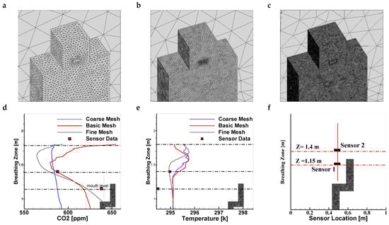
Figure 2.
Mesh study. (a–c) Coarse, basic, and fine mesh. (d,e) Comparison between coarse, basic, and fine mesh profiles and sensors measured data. (d) CO2 concentration. (e) Temperature. (f) Sensors’ location at BZ height.
Figure 2 indicates the comparison between the coarse, basic, and fine meshes. The variation between results at the BZ line for the basic and the fine mesh was within acceptable limits for both CO2 and temperature, indicating that the basic mesh was sufficient for further study (Figure 2d–f). It can be seen that at the BZ level close to the occupant’s BZ, the basic and fine meshing schemes show good agreement for both CO2 and temperature. However, at higher elevations, the data show differences between the basic and fine mesh. Since the analyses in our study primarily focused on the BZ, the basic mesh scheme was selected to achieve a balance between computational cost and accuracy of the results.
2.3. Model Validation
To measure the variables, vertical lines 1 and 2 (Figure 1a) and horizontal lines a, b, c, and d (Figure 1b) were drawn as reference axes intersecting the sensor locations. The steady-state simulated CO2 concentration was evaluated by comparing it to the average CO2 measurements recorded by sensors positioned at corresponding locations, as shown in Figure 1, and described in the experimental setup. Figure 3 illustrates the average measured temperature and CO2 concentration at the sensor locations (Figure 1) in the unoccupied experimental test room over a three-month period, along with the results from the steady-state CFD simulation. Figure 3a–f show the discrepancies between simulated data and measured data at the sensor point locations. The mean absolute error between the temperature data from sensors and the simulation was 1 °C and 1.2 °C for sensors at lines 1 and 2, respectively. Outdoor CO2 fluctuations, not thoroughly mixed conditions, affected the experimental environment, and the sensor data show deviations from the simulated data. The simulated data were within acceptable accuracy with the experiment results for further study and modeling other room conditions. The results shown in this section are limited to model validation, not the actual results from the broader range of simulations.
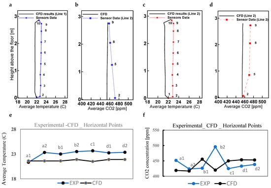
Figure 3.
Comparison of CFD simulated and experimental measurements data at the arranged sensor positions shown in Figure 1. (a,b) Temperature and CO2 level at line 1. (c,d) Temperature and CO2 level at line 2 (the mean absolute error for air temperature was about 1 °C in panel a, and about 1.2 °C in panel (c). (e) Temperature at horizontal point locations. (f) CO2 concentration (ppm) at horizontal locations.
2.4. The Procedure for Calculating Ventilation Effectiveness
Ventilation effectiveness has been a key focus of several studies, with various quantification methods discussed in the literature. Kato et al. (1988) examined three stages for ventilation efficiency to evaluate the distribution of ventilation effectiveness in a room []. One traditional method of determining mean ventilation effectiveness is to average contaminant concentrations measured at the breathing level and utilize distributed tracer gas sources throughout the room [,]. The mean ventilation effectiveness (VE) is defined based on European Committee for Standardization (EN 16798-3:2017) and contaminant removal effectiveness in REHVA Guidebook No 2 [,]. Sandberg (1981) [] introduced both relative and absolute definitions of VE, which have since been incorporated into ASHRAE guidelines []. To calculate the maximum amount of pollutant present and the actual effectiveness of the system when exposed to the maximum concentration of contaminants, the absolute VE was measured. In a recent study, Kurnitski et al. (2023) [] applied the concept of point-source ventilation effectiveness for the breathing zone. They recommended that only the top 50% of measurement points with the highest contaminant concentrations be considered when evaluating VE []. However, in practical situations, occupants are in different arrangements and are not always in the maximum contaminant concentration zone. Therefore, this study aims to assess Relative Ventilation Effectiveness to determine ventilation performance and how efficiently the ventilation system removes indoor air contaminants in an office room. In this context, Relative Ventilation Effectiveness deals with the average of absolute concentration at any point in space, where concentration measurements were taken along the breathing line. The primary objective was to evaluate how well different ventilation system configurations and zonal arrangements affect air distribution and contaminant removal, especially at the critical breathing zone for variable occupancy levels. Average CO2 concentration was measured along the breathing zone (at 0.75–1.8 m, Figure 2f) to capture the dynamic behavior of contaminant concentration and calculate ventilation effectiveness, based on the definition of the breathing zone (BZ) in ANSI/ASHRAE Standard 62.1 [].
The relative ventilation effectiveness is defined in an Equation (2) obtained from ASHRAE RP-1833 (2023) []:
is the ventilation effectiveness, represents the concentration in the exhaust, denotes the average concentration at the point j, and is the concentration at the supply. The CO2 levels in the room vary across the different areas. To analyze the effectiveness of system settings and measure each zone’s VE, the room was divided into five zones based on the seating arrangement and the occupants’ distance from the nearest dominant supply, corresponding to the total number of occupants. A dominant inlet is defined as the inlet with the most significant impact on the occupants in each zone.
Figure 4 show the room with three occupancy patterns and five zones. Having more than one point of interest in investigating the effectiveness of the studied room ventilation, Equation (2) was expanded to Equation (3) to consider all the different zones in the overall VE. The distance separating each zone for measuring zonal VE was calculated based on the dominant diffuser’s influence.
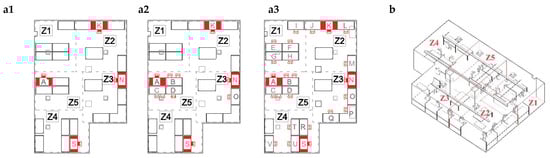
Figure 4.
(a1–a3) Experiment room with three occupancy patterns. (b) The experiment room with five distinct zones.
The mean CO2 concentration in each occupant’s BZ in each zone for all arranged occupant seating, as shown in Figure 4, was recorded. CO2 concentration levels were used to measure the system’s ability to dilute contaminants. The maximum recorded CO2 concentration in each zone was representative of the lowest effectiveness and was selected as an indicator for measuring the absolute ventilation effectiveness for each zone. BZ air quality was measured at each zone, with the number of samples equal to the number of occupants’ breathing zones. The peak concentration at BZ was averaged to represent the single largest value (Ci), which was substituted in Equation (3). Hence, the difference in contamination concentration between the maximum value at the BZ at each zone and the supply for each zone was used for the calculation. The mean difference in concentrations for all zones was the sum of the differences in absolute zonal contamination concentration as compared to the respective concentration at supply, averaged over all five zones, which is the denominator in Equation (3). The relative ventilation effectiveness in a room was defined as the ratio of the difference between contamination concentration at the exhaust and average concentration at the supply to the mean zonal difference in concentration (Equation (3)).
, , and represent the average concentration in the exhaust for the whole room, the average concentration in the supply for the entire room, and the average of the absolute (maximum) recorded concentrations at the breathing level, respectively.
2.5. Effect of Various Layouts on Air Quality and Ventilation Effectiveness
After developing a validated simulation method for this study, subsequent simulations in CFD were developed considering several variables. The reference case was simulated with 2.9 m (9.5 ft) of ceiling height, actual air supply rates, and two different locations of exhaust vents. Additional simulations were conducted for ceiling heights of 3.2 m (10.5 ft) and 2.6 m (8.5 ft), three different occupancy loads, and various additional ACH rates. Table 4 summarizes all the simulation cases in the current study: 17 simulation models to compare ventilation effectiveness across different study variables. This study seeks insights into optimal ventilation strategies based on system layouts and arrangements. The nomenclature of the cases was derived in the following way. Cases 1, 2, and 3 represent the reference ceiling height of 2.9 m, 3.2 m, and 2.6 m, respectively. “a” and “b” represent the exhaust locations axis at the side and the middle of the room, respectively, as shown in Figure 1. In Table 3, the numbers 1, 2, and 3 represent the number of occupants, 4, 10, and 24, respectively. A constant air change rate of 3.06 ACH for baseline comparisons was considered. Additional tests were performed with reduced air change rates. The ventilation rate was summarized in terms of ACH, calculated using Equation (4) [].
Table 4.
Parametric study matrix for each type of indoor ceiling height, number of occupants, and air change rate.
As can be seen from Table 4, two different ACH levels were examined. The baseline ACH was 3.06, as described in Table 1. When the ceiling height was changed, i.e., the room volume was changed, the supply airflow rate was also adjusted to keep the ACH at the base case level for model Case 2-a3. Then, the air supply rates were kept constant as the reference model, and the ceiling height was changed (i.e., change in room volume) to reduce the ACH, which are shown as models described with RACH at the end of their names. Finally, for a smaller ceiling height, the supply flow rate was also reduced to achieve the same level of ACH for Case 3-a1 and Case 3-b1.
Indoor air quality was evaluated at each zone using the mass fraction of CO2 (which can be converted to ppm when multiplied by 106). Moreover, six different seating arrangements with respect to the supply elements were examined to evaluate their impact on BZ air quality. These seating arrangements can be found in Figure 5a: (a) facing directly to the seating, (b) diagonally facing to seating: the supply diffuser is at a diagonal direction to the vertical plane in the forward direction of the occupant, (c) side to side arrangements: the supply diffuser is located normal to the vertical plane along the forward direction of the occupant’s mouth, (d) diagonally back to the seating (e) directly behind the seating, and (f) above the seating. The occupant’s orientation with respect to the wall is shown in Figure 5b: (1) facing the forward wall, (2) corner arrangement, and (3) parallel to the wall.
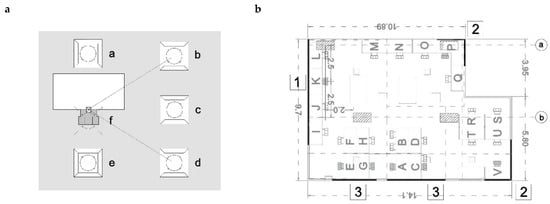
Figure 5.
(a) Six orientations, arrangements a, b, c, d, e, and f, with respect to the supply elements. (b) Occupant’s orientation with respect to the wall: (1) facing the wall; (2) seating at corners; (3) positioned parallel to the wall.
3. Results
Results indicate that the same airflow rate settings can improve indoor air quality without the need for excessive ventilation rates, thereby avoiding additional energy consumption. However, despite acceptable room-average concentrations, localized CO2 accumulation was observed in the breathing zone, where concentrations approached critical thresholds []. Rearranging occupants, as well as optimizing the placement of diffusers and exhausts, is therefore necessary to improve zonal ventilation effectiveness.
3.1. Impact of System Settings on Efficient Improvement of Air Quality
Figure 6, Figure 7 and Figure 8 show CO2 distribution across ceiling heights (2.6, 2.9, 3.2 m) and exhaust locations (‘a’ and ‘b’ axes, Figure 1a) with 4, 10, and 24 occupants. At lower occupancy (<10), system settings generally maintain acceptable IAQ []. Figure 6a–c illustrate CO2 patterns for four occupants (A, K, N, S; Figure 4a) under different ceiling and exhaust setups. The four occupants were selected to capture IAQ variations: A (Z5) parallel to a wall, K (Z2) close to the exhaust, N (Z3) between two exhausts, and S (Z4) placed far distant from both supply and exhaust.
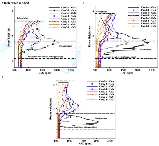
Figure 6.
Comparison between exhaust locations “a” and “b” axis on air quality for the model with four occupants. (a) in Case 3 (ceiling height 2.6 m), (b) Case 1 (ceiling height 2.9 m), and (c) Case 2 (ceiling height 3.2 m).
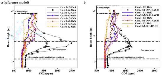
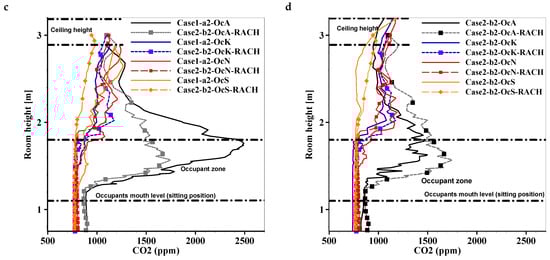
Figure 7.
Profiles of CO2 concentration for various layout settings in a room with 10 people. (a) Comparison between “a” and “b” exhaust axes in Case 1 models. (b) Comparison between ceiling heights when exhaust is located at “b” axis. (c) Comparison between “a” and “b” exhaust axes for Cases 1 and 2. (d) Comparison between reference ACH and reduced ACH (RACH) for Case 2 (ceiling height 3.2 and “b” exhaust axis).
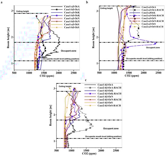
Figure 8.
O2 concentration profiles across different room layouts with 24 occupants. (a) Comparison between “a” and “b” exhaust axes in the room with reference to the ceiling height. (b) Comparison between the air quality for the same and reduced air change rate for a room with 3.2 m ceiling height and exhaust on “a” axis. (c) Comparison between ceiling heights when exhaust is located at “b” axis (under the same and reduced air change rate, RACH).
It can be seen from Figure 6a that the system does not work properly in Case 3, which has a 2.6 m ceiling height. The contamination levels in the BZ surpass those observed in the reference model for both models with exhaust locations at “a” and “b” axes (Figure 6a,b). In Case 3 (2.6 m ceiling), CO2 levels at the BZ height range from 620 to 750 ppm, compared to 550–690 ppm in the reference case (Figure 6a–b). Despite having the same ACH and number of occupants as Case 1 and Case 2, Case 3 exhibits the poorest air quality among the models with four occupants. With the same inflow air, increasing the ceiling level by 30 cm from Case 3 to the reference model, the air quality improves by 13% for occupant A and 5% for occupants N and S. However, near the exhaust, Case 3 indicates better air quality than the reference model (Occupant K). Case 3 was excluded from the VE calculations for the 10 and 24-occupant models due to elevated CO2 concentrations at the mouth level compared to the corresponding cases with increased ceiling height (Figure 6a).
In cases with low occupancy density, seats near the exhaust (K and N) experience improvement in air quality at the breathing zone (BZ) compared to other positions. The occupant at seat K is exposed to impaired air quality with CO2 contamination elevated by 14% (from 600 to 800 ppm) when the exhaust arrangement is changed from “a” axis to “b” axis (Figure 6b). The role of higher ceilings in shifting CO2 gradients from the BZ to upper levels in the room was significant, as shown in Figure 6c. According to the reference model (Case 1), as the number of people increases, the indoor CO2 concentration rises almost proportionally when the ventilation rate remains constant, as can be seen from Figure 6, Figure 7, and Figure 8. The CO2 concentration ranges between 600 and 700 ppm, 800 and 900 ppm, and 1300 and 1400 ppm in the reference cases with 4, 10, and 24 people, respectively. The distribution of CO2 is also closely tied to occupancy levels, and doubling the occupants roughly doubles the indoor CO2 elevation. At lower occupancy levels (<10 persons) and with ceiling heights ≥2.9 m, the system settings were generally sufficient to maintain indoor CO2 concentrations below 1000 ppm, the commonly accepted threshold for acceptable air quality (48). Figure 7a–c show the contaminant distribution for each system’s design configuration when 10 people occupied the room, illustrating the change in CO2 distribution at the BZ for occupants A, K, N, and S.
As shown in Figure 7a, Case 1, where the exhaust vent is located along the “b” axis, the contaminant concentration for occupants K and N is higher compared to the case with the exhaust on the “a” axis. Specifically, the concentration at BZ elevated by approximately 10% (from 829 to 916 ppm) for occupant K and 6% (from 920 to 984 ppm) for occupant N. However, changing the exhaust location from the “a” to the “b” axis reduces the contaminant by 28% and about 4% (from 895 to 854 ppm) for occupants A and S, respectively. When the room is occupied with fewer individuals, the ventilation system works more efficiently in removing contaminants, particularly when occupants are positioned near the exhausts (occupants K and N). This finding is in line with our previous study []. In Figure 7b, it is shown that increasing the ceiling height while keeping the exhaust position at the “b” axis results in lower contaminant levels at BZ in Case 2, even though maintaining the same air flow rate as in Case 1, resulting in reduced ACH due to the larger volume. In this case, at the same air flow rate, increasing the ceiling level by about 10% in Case 2 (from 2.9 m to 3.2 m) improved air quality at BZ for occupants at A, K, N, and S positions compared to Case 1, with an average improvement of approximately 10%. Comparing the results of Case 2 to the reference model (Case 1), Figure 7c demonstrates that increasing the ceiling height by 10% while relocating the exhaust at the “b” axis significantly improves the air quality in Case 2 compared to the reference model (Case 1). On average, air quality at the A, K, N, and S positions improved by 148 ppm, equivalent to a mean reduction of 11.6% (1046 ppm to 900 ppm).
It was interesting to note that with the increase in ceiling height (i.e., increasing the room volume), the air change rate was not solely the determining factor in maintaining air quality (Figure 7d). Figure 7d shows that, in models with a ceiling height of 3.2 m, comparison between the reference ACH (3.06) and reduced air change rate (RACH) indicates an average CO2 decrease of approximately 8% with RACH at the breathing zones of occupants A, B, and D, while occupant N exhibited no appreciable change. Moreover, the results show that even with a reduced air change rate, comparable air quality can be maintained at the breathing zone. It is also worth mentioning that relocating the exhaust vent has a greater effect on improving air quality for occupants sitting far from the exhaust (location A) than increasing the ceiling height. In contrast, the elevated contaminants were noticed for the occupant located at position K in Case 2-b2. The reason behind this phenomenon is possibly attributable to the reduced time requirement for the contaminants to exit the control volume, owing to the proximity of the exhaust from all the users being considered compared to the side exhaust setting. The contaminant distribution for each system layout when the room is occupied with 24 people is shown in Figure 8a–c, with the CO2 concentration distribution at the BZ for seats A, K, N, and S.
Figure 8a (Case 1) compares the contaminant concentration at the BZ for models with exhaust locations along the “a” and “b” axes. Locating the exhaust on the “b” axis led to an average 6.2% decrease in contaminant concentration at the breathing zones of occupants A, K, N, and S from 1348 to 1278 ppm (Case 1). According to previous models, an improved air quality is expected with increasing ceiling height in model Case 2-a3. However, when the ceiling height increases from 2.9 m to 3.2 m (10%), the air quality of Case2-a3 is relatively poorer for occupants K and N, who sit close to the exhausts (Figure 8b). Figure 8b shows that, despite the increased air change rate in Case 2-a3, CO2 concentrations remain elevated compared to Case 2-b3-RACH, where reduced airflow, combined with an optimized exhaust location, reduced the CO2 concentration by 140 ppm. In Case 2-a3, the higher ceiling and ‘a’ axis exhaust diminish the driving force of air stream vectors, weakening contaminant removal and worsening air quality near the exhaust.
A higher value of air flow rate (0.339 m3/s instead of 0.311 m3/s in the reference case) was applied to Case 1-b3 (Figure 8c), leading to reduced contaminants at the BZ to below the standard CO2 threshold of 1000 ppm for a 24-occupant model for occupants at A, K, N, and S positions. Although the contamination concentration decreased at an increased mass flow rate in Case 1-b3, a supply flow rate of 0.311 m3/s (RACH = 2.8), combined with the higher ceiling height (Case 2-b3-RACH, Figure 8c), resulted in even lower contaminant concentration. This result indicates that selecting a ceiling at a higher level can improve air quality in rooms with lower ACH when the exhaust is efficiently located. At the breathing zone, occupants K, N, and S in Case 2-b3-RACH experienced an average contaminant reduction of 4.6% compared to Case 1-b3, while the occupant at location A experienced a 19% increase. This outcome is possibly attributable to stagnancy and the lock-up phenomenon [], in which ventilation remains ineffective in certain parts of the room. Consequently, it highlights the importance of careful planning and design of occupant arrangements in relation to system settings for enhanced air quality and improved ventilation effectiveness.
Figure 9 indicates the contours of CO2 concentration across the horizontal plane at the breathing level (1.15 m above the floor) for the reference case (Case 1) with three occupancy patterns, and the 24 occupants’ models with increased ceiling height and both exhaust locations (Case 2-a3 and Case 2-b3). As can be seen in Figure 9a–c, increasing the number of occupants increases the CO2 concentration in some parts of the room in the reference model. Figure 9d indicates that for the Case 2-a3 model, the system layout does not appropriately dilute the BZ contaminants. The occupant thermal plume direction, which is affected by indoor driving forces and convection is a key factor in BZ air quality []. Thus, Figure 9e indicates that changing the system layout from Case 2-b3 improves air quality at BZ by enhancing the indoor air mixing, compared to the same case with an increased ACH (Figure 9c).
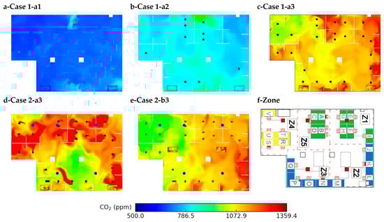
Figure 9.
The CO2 concentration at various system layouts and direction of thermal plume. (a–c) Reference model with three occupancies of 4, 10, 24. (d) Case 2-a3. (e) Case 2-b3. (f) Occupancy arrangements.
3.2. Impact of Occupant Seating Orientations on Efficient Improvement of Air Quality
The CO2 concentration at BZ for various seating arrangements and orientations, as shown in Figure 10a–e, was analyzed for cases with 24 occupants (Case 1-a3 and Case 1-b3) to study the impact of occupants’ arrangement and orientations, presented in Figure 5, on measured air quality. Occupants D (arrangement ‘c’) and T (arrangement ‘e’) are equidistant from supply and exhaust but differ in their arrangement (Figure 10a). Despite 1% lower airflow, the ‘c’ arrangement yielded 7.3% better air quality (1205 vs. 1260 ppm) as its parallel supply more effectively targeted the BZ.
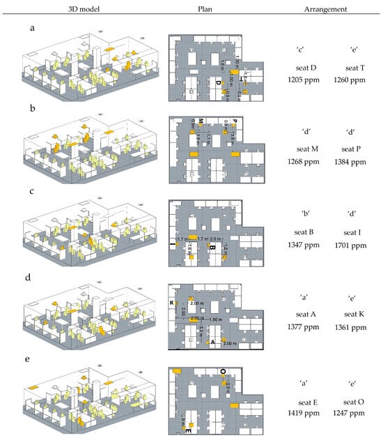
Figure 10.
(a–e) Case 1-a3 and Case 1-b3 with 24 occupants, the effect of orientation on the BZ air quality.
Seats M and P are diagonally equidistant from the diffuser with ‘d’ arrangement (Table 5) but differ in wall orientation. Occupant P, seated in the corner, experiences elevated contaminant levels compared to occupant M (about 8.7%), positioned at the center of the room, even with greater supply airflow in Zone 3 (Figure 10b).
Table 5.
The CO2 concentration at BZ for various seating arrangements positioned at equidistance from the supply and exhaust vents.
Occupants at seat I (arrangement ‘d’) and occupant seated on the right side of location B (arrangement ‘b’) are equidistant from supply and exhaust. Seat B, centrally located between two suppliers and exhausts, shows 26.3% better air quality than seat I. When the diffuser is diagonally distant, BZ contaminant levels are lower for occupants facing the supply (‘b’) than for those with it at their back (‘d’) (Figure 10c). In Case 1-b3 (Figure 10d, Table 5), seats A (X = 3.2, Y = 1.5 m) and K (X = 2.5, Y = 2 m) are similarly positioned relative to the supply. Seat A is closer to the wall (0.5 m vs. diffuser at 0.8 m) and shows elevated contaminants than seat K (arrangement ‘e’), as the near-wall placement traps pollutants [owing to the locked-up phenomenon, as described in []. A similar effect appears in seats O and E (Figure 10e): despite 4% lower airflow at O, its air quality is 12% better than E due to spatial configuration.
Seats J and M have approximately similar distances to the exhaust, but placement M shows 62.1% better air quality than J, primarily due to its proximity to the diffuser (Figure 5b). Seat N (Z3) is positioned between two opposing diffusers, neutralizing supply air speed. A similar effect occurs in placement A and B (Z5), where airflows from two diffusers collide. In Case1-b3, Occupant S (z4) has a similar distance to the supply and exhaust as occupant at seat I (z1). However, occupant S experiences 36% less contaminant concentration than occupants at seat I, as it faces the supply diagonally.
A and E are arranged similarly to the wall and supply diffuser (Figure 5b, Table 5). Although E is closer to the supply, it has poorer air quality. The optimum distance to the supply diffuser regarding the airflow rate also plays a key role in better BZ air quality and the effectiveness of the system in delivering fresh air.
3.3. Zonal Ventilation Effectiveness and System Performance
The mean CO2 concentration at each exhaust vent for each simulated model is presented in Table 6 for calculating the ventilation effectiveness of each layout. This table shows the average concentration of CO2 at the BZ for occupant A, as a reference to indoor air quality.
Table 6.
The average CO2 concentration at BZ for occupant A and the exhaust vents.
The zonal ventilation effectiveness, calculated using Equation (3), is shown in Figure 11. This graph illustrates how ceiling height level or exhaust vents can result in altered air quality metrics and the performance of the ventilation system, depending on the orientation of the occupants and the air distribution, rather than just controlling the ACH.
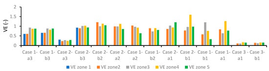
Figure 11.
Zonal Ventilation Effectiveness for studied cases (Zone 1 is only occupied in a fully occupied room).
Figure 11 indicates ventilation effectiveness for each defined zone, as identified in Figure 4. Contaminant removal varies with system layout and seating arrangements, as each zone has distinct supply and exhaust distances. The supply diffuser has been identified as the primary driver influencing the efficiency of contaminant removal []. Therefore, average distances between occupants and the supply were examined to evaluate zonal effectiveness under full occupancy (Table 7).
Table 7.
Occupant’s arrangement type and the average distance regarding to effective supply in each zone.
As can be seen from Table 7, Zones 2 and 3 each accommodated four people with the same arrangement relative to supply and wall (Figure 5). However, Zone 3 showed better VE because the diffuser was closer to the occupants. As the average distance increased from 1.4 m in Zone 3 to 2.2 m in Zone 2 (vertical distance 1.1–2.2 m), VE decreased by 40%, indicating sub-optimal air distribution in Zone 2. In the 10-occupant cases, occupant density has a strong influence on VE, with Zone 2 performing 20% better than Zone 3. With fewer occupants in Z2 (one) than Z3 (two), VE in Z3 is driven more by density than supply proximity (Figure 4(a2)). Higher occupancy diminishes VE, suggesting required dynamic airflow adjustment to zonal occupancy density.
In Zones 1, 4, and 5, occupants are seated at the perimeter of a rectangular shape (boardroom arrangement). Among all the zones shown in Figure 11, analysis of the normal density distribution revealed that Zone 4 had consistently higher VE values, followed by Zones 3, 2, 5, and 1 (Figure 12).
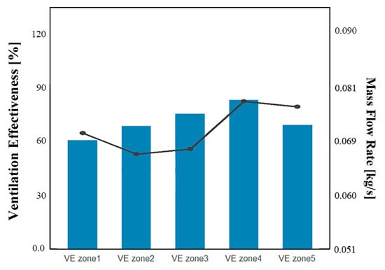
Figure 12.
The average of VE and the corresponding supply flow rate for each zone across all studied models.
Figure 12 shows VE and mass flow across five zones. Blue bars denote the average VE, and black lines represent the mass flow rate for each zone. Zone 4 has the highest VE, with a high supply mass flow, while Zones 1 and 5 exhibit lower VE despite moderate flow, indicating inefficiencies in airflow distribution. With 8% higher supply, Zone 4 achieves 26% better VE than Zone 1.
Higher VE despite lower flow in Zones 2 and 3 highlights the role of room layout and occupant arrangement over supply rate. Though Zones 2 and 3 have lower flow and greater occupant–supply distance than Zones 1 and 5, they still outperform them in VE (Figure 12). These findings suggest that the underlying mechanism of airflow distribution, with respect to occupant positioning, the flow distribution, and mixing of primary and secondary flow regimes, has a more significant impact on the ventilation system’s performance. These results also suggest that the well-mixed assumption is not sufficient, especially when multi-occupancy spaces are considered, and the supply flow rate should be adjusted with the respective understanding of flow distribution in relation to occupant arrangements. Similarly, the occupant arrangement can also be designed based on the system’s characteristics to optimize the system’s performance in distributing the ventilated air streams.
In Zone 4, the seating–supply arrangement (‘a’, ‘e’, ‘c’ for seating R, T, V) produced the most effective contaminant removal at the BZ. Separation from the indoor mixed air further increased VE in Zone 4. Although Zones 1 and 4 have the same occupant density (five occupants), Zone 4 achieved higher VE despite a greater average occupant–supply distance (Table 7). In Zone 1, the diffuser above the desk near the wall (arrangement ‘a’, ‘b’, ‘d’) reduced VE, as seat I (‘d’) and seats E and G were affected by lock-up phenomena []. Occupants positioned parallel to the wall at 0.5 m experienced adverse pressure and pollutant accumulation (seats G and E). By contrast, Zone 5 achieved improved VE due to arrangements that enhanced contaminant removal at the BZ (51).
Figure 13 shows the room VE for all cases. As occupant numbers rise, VE equations (CO2 at BZ and exhaust) cannot be directly compared across cases. With the same supply, a 3.2 m ceiling (Case 2) generally yields higher VE than a 2.9 m ceiling (Case 1), for both side and middle exhaust. Improvements include 20% (Case 2-b3), 24% (Case 2-b2), and 74% (Case 2-b1) over the corresponding Case 1-b models. This indicates that increasing control volume does not require more air supply to meet the target air quality. This observation is most likely due to better air mixing with increased control volume, and increasing the supply velocity does not necessarily result in better mixing. Rather, this finding corroborates the fact that a lower quantity of supply air can achieve better air quality if the distribution can be optimized by different methods (e.g., changing the exhaust location or increasing the control volume). Increasing the ceiling height in the mixing ventilation system allows the thermal plumes to rise higher before interacting with the supply of fresh air and mixing with the air distribution. Proper diffuser placement, supply flow rate, and flow direction are crucial for the VE. The optimized layout (Case 2-b3) improves VE by ~23% over Case 1-a3. Combining this layout with optimized seating reduces the need for higher airflow and ACH, which leads to energy savings.
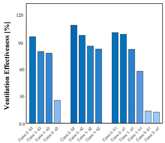
Figure 13.
Room Ventilation Effectiveness for all studied cases.
4. Limitations
The model and the system analyzed in this study were based on the steady state model, but dynamic factors like fluctuating occupancy levels and real-time changes in pollutant sources have not been taken into account. The occupants of the experimental facility might have different levels of CO2 generation based on their gender and age. However, this study considered the same amount of CO2 generation. Furthermore, although occupants in the room have different heights, all the occupants in this study are considered to have the same height to be able to compare concentrations at BZ.
The combined effects of these factors in varied architectural configurations, particularly in spaces with non-standard ceiling heights, complex geometries, or high occupant density, were out of scope for this study. Moreover, the temperature profile affects CO2 stratification, the effect of which has not been considered in this study. Ventilation effectiveness equation (Equation (2)) for absolute measurements could not be used to compare VE for different occupancy patterns in different models. Instead, the absolute measurements were used for comparison of zonal ventilation effectiveness in each case.
5. Conclusions
In this study, different settings of a mixing ventilation system (such as ceiling height, exhaust vent location, supply airflow rates, and occupancy patterns and arrangements) in a shared office space were studied to measure ventilation effectiveness using validated CFD simulations. This study used the exhaled CO2 in a densely occupied space as an indicator of air quality. The specific conclusions from this study are as follows:
- Airflow rate is not an indicator of air quality. A well-mixed assumption in a mixing ventilation system is not sufficient. Careful planning of occupant arrangement in relation to the system settings leads to an improved air quality and increased ventilation effectiveness. An optimally located side-to-side arrangement with respect to a supply diffuser resulted in 26.3% better air quality compared to the supply to the back arrangement.
- The number of occupants carries a significant weight in determining ventilation effectiveness. The VE is primarily influenced by occupant arrangement and density rather than supply proximity (location and flow rate). However, both variables affect VE.
- Exhaust location has a greater impact on efficient air quality improvement than ceiling height in system design. Placing the exhaust in the middle of the room (at an equal distance to all the contaminant sources) resulted in up to 10% improvement in ventilation effectiveness. Simultaneously, increasing the ceiling height by 10% improved ventilation effectiveness by 20% in a fully occupied room. This improvement yielded an 8.5% reduction in the required air change rate in the model with exhaust at the “b” axis.
- A higher ceiling height combined with a lower airflow rate can achieve nearly the same improvement in air quality as the increased airflow rate. In the same airflow rate, increasing the ceiling level improves the air quality in the breathing zone and VE by approximately 20% in a fully occupied room.
- In low-density rooms (<10 occupants), proximity to exhausts enhanced breathing zone air quality, particularly at lower ceiling heights, whereas in high-density rooms (24 occupants), the same exact positioning resulted in both lower air quality and lower ventilation effectiveness.
- Positioning a supply diffuser too close to a wall (≈0.8 m) with an occupant seated parallel to the supply diffuser at a distance of 0.5 m promoted an adverse pressure gradient, causing contaminant accumulation in the breathing zone. Maintaining a horizontal distance greater than 90 cm yielded more favorable airflow patterns and improved air quality.
- The effectiveness of mixing ventilation systems depends on how the circulation flow interacts with the thermal plume from the occupants, the thermal plume direction, and the subsidence of fresh air at BZ.
Ventilation effectiveness is primarily related to the number of people (their proximity), their arrangement in relation to the supply and supply proximity, flow direction (11), direction of the thermal plume, layout of the exhaust vent, and ceiling height, which affects the room’s convection. In the future, the research team plans to expand this study with dynamic simulations to understand the dynamic event impacts on the CO2 generation and ventilation effectiveness. Moreover, multi-occupancy spaces such as classrooms, where elevated CO2 contributes to sleepiness and reduced alertness, and balancing comfort with energy use remains a challenge, which needs to be further investigated.
Author Contributions
Conceptualization, A.B.; Methodology, M.L., S.C. and A.B.; Software, S.C.; Validation, A.B.; Formal analysis, M.L.; Investigation, M.L., S.C. and A.B.; Data curation, M.L. and A.B.; Writing—original draft, M.L.; Writing—review and editing, S.C. and A.B.; Supervision, A.B.; Funding acquisition, A.B. All authors have read and agreed to the published version of the manuscript.
Funding
This research was supported by Louisiana State University internal funding under the Student Technology Fee funding.
Data Availability Statement
The original contributions presented in this study are included in the article. Further inquiries can be directed to the corresponding author.
Conflicts of Interest
The authors declare that they have no known competing financial interests or personal relationships that could have appeared to influence the work reported in this paper.
Nomenclature
| Symbol/Abbreviation | Definition | Unit |
| ACH | Air Changes per Hour | h−1 |
| AME | Absolute Mean Error | - |
| A | Area (inlet/exhaust) | m2 |
| BZ | Breathing Zone (typically 0.75–1.8 m above floor level) | - |
| CFD | Computational Fluid Dynamics | - |
| CO2 | Carbon dioxide (used as tracer gas/contaminant proxy) | ppm |
| h | Ceiling height | m |
| HVAC | Heating, Ventilation, and Air Conditioning | - |
| ṁ | Mass Flow Rate | kg/s |
| ppm | Parts per million | - |
| q″ | Heat Flux (surface heat transfer rate per unit area) | W/m2 |
| Q | Volumetric airflow rate | m3/s or CFM |
| T | Air temperature | °C or K |
| U | Air velocity | m/s |
| VE | Ventilation Effectiveness | - |
| η | Efficiency | - |
| ρ | Air density | kg/m3 |
| H2O (v) | Water vapor concentration | g/kg (humidity ratio) %RH |
References
- ASHRAE. ASHRAE Handbook—Fundamentals, 2017th ed.; American Society of Heating, Refrigerating and Air-Conditioning Engineers: Atlanta, GA, USA, 2017. [Google Scholar]
- Awbi, H.B.; Gan, G. Evaluation of the Overall Performance of Room Air Distribution. In Proceedings of the 6th International Conference on Indoor Air Quality and Climate, Helsinki, Finland, 4–8 July 1993. [Google Scholar]
- Sandberg, M. What Is Ventilation Efficiency? Build. Environ. 1981, 16, 123–135. [Google Scholar] [CrossRef]
- Behne, M. Indoor Air Quality in Rooms with Cooled Ceilings. Mixing Ventilation or Rather Displacement Ventilation? Energy Build. 1999, 30, 155–166. [Google Scholar] [CrossRef]
- Jameson, A.; Baker, T.J. Improvements to the Aircraft Euler Method; AIAA Aerospace Research Central: Reston, VA, USA, 2012. [Google Scholar]
- Rajashekaraiah, T.; Panigrahi, S.P.; Sanjai, G.S.; Dulabhai, H.P.; Vijaykumar, V.M. Investigating Various Meshing Techniques in Computational Fluid Dynamics (CFD) for Their Impact on Heat Transfer Parameters of Fins. J. Mines Met. Fuels 2025, 73, 117–128. [Google Scholar] [CrossRef]
- Pantelic, J. Designing for Airborne Infection Control; ASHRAE: Atlanta, GA, USA, 2019. [Google Scholar]
- Zhang, S.; Lin, Z. Dilution-Based Evaluation of Airborne Infection Risk—Thorough Expansion of Wells-Riley Model. Build. Environ. 2021, 194, 107674. [Google Scholar] [CrossRef]
- Rencken, G.K.; Rutherford, E.K.; Ghanta, N.; Kongoletos, J.; Glicksman, L. Patterns of SARS-CoV-2 Aerosol Spread in Typical Classrooms. Build. Environ. 2021, 204, 108167. [Google Scholar] [CrossRef]
- Li, W.; Chong, A.; Hasama, T.; Xu, L.; Lasternas, B.; Tham, K.W.; Lam, K.P. Effects of Ceiling Fans on Airborne Transmission in an Air-Conditioned Space. Build. Environ. 2021, 198, 107887. [Google Scholar] [CrossRef]
- Wang, F.; Permana, I.; Rakshit, D.; Prasetyo, B.Y. Investigation of Airflow Distribution and Contamination Control with Different Schemes in an Operating Room. Atmosphere 2021, 12, 1639. [Google Scholar] [CrossRef]
- Chung, K.-C.; Hsu, S.-P. Effect of Ventilation Pattern on Room Air and Contaminant Distribution. Build. Environ. 2001, 36, 989–998. [Google Scholar] [CrossRef]
- Van Hooff, T.; Blocken, B. Mixing Ventilation Driven by Two Oppositely Located Supply Jets with a Time-Periodic Supply Velocity: A Numerical Analysis Using Computational Fluid Dynamics. Indoor Built Environ. 2020, 29, 603–620. [Google Scholar] [CrossRef]
- Memarzadeh, F.; Xu, W. Role of Air Changes per Hour (ACH) in Possible Transmission of Airborne Infections. Build. Simul. 2012, 5, 15–28. [Google Scholar] [CrossRef]
- Liu, S.; Koupriyanov, M.; Paskaruk, D.; Fediuk, G.; Chen, Q. Investigation of Airborne Particle Exposure in an Office with Mixing and Displacement Ventilation. Sustain. Cities Soc. 2022, 79, 103–718. [Google Scholar] [CrossRef]
- Cao, G.; Awbi, H.; Yao, R.; Fan, Y.; Sirén, K.; Kosonen, R.; Zhang, J. A Review of the Performance of Different Ventilation and Airflow Distribution Systems in Buildings. Build. Environ. 2014, 73, 171–186. [Google Scholar] [CrossRef]
- Qin, C.; He, Y.; Li, J.; Lu, W.Z. Mitigation of Breathing Contaminants: Exhaust Location Optimization for Indoor Space with Impinging Jet Ventilation Supply. J. Build. Eng. 2023, 69, 106250. [Google Scholar] [CrossRef] [PubMed]
- Hongtao, X.; Naiping, G.; Jianlei, N. A Method to Generate Effective Cooling Load Factors for Stratified Air Distribution Systems Using a Floor-Level Air Supply. HVAC R Res. 2009, 15, 915–930. [Google Scholar] [CrossRef]
- Berlanga, F.A.; Olmedo, I.; de Adana, M.R.; Villafruela, J.M.; José, J.F.S.; Castro, F. Experimental Assessment of Different Mixing Air Ventilation Systems on Ventilation Performance and Exposure to Exhaled Contaminants in Hospital Rooms. Energy Build. 2018, 177, 207–219. [Google Scholar] [CrossRef]
- Park, J.; Lee, K.S.; Park, H. Optimized Mechanism for Fast Removal of Infectious Pathogen-Laden Aerosols in the Negative-Pressure Unit. J. Hazard. Mater. 2022, 435, 128978. [Google Scholar] [CrossRef]
- Wang, C.; Hong, J. Numerical Investigation of Airborne Transmission in Low Ceiling Rooms under Displacement Ventilation. Phys. Fluids 2023, 35, 023321. [Google Scholar] [CrossRef]
- Hunt, G.R.; Linden, P.F. Displacement and Mixing Ventilation Driven by Opposing Wind and Buoyancy. J. Fluid Mech. 2005, 527, 27–55. [Google Scholar] [CrossRef]
- Izadyar, N.; Miller, W. Ventilation Strategies and Design Impacts on Indoor Airborne Transmission: A Review. Build. Environ. 2022, 218, 109158. [Google Scholar] [CrossRef]
- Katramiz, E.; Ghaddar, N.; Ghali, K.; Al-Assaad, D.; Ghani, S. Effect of Individually Controlled Personalized Ventilation on Cross-Contamination Due to Respiratory Activities. Build. Environ. 2021, 194, 107719. [Google Scholar] [CrossRef]
- Ai, Z.; Hashimoto, K.; Melikov, A.K. Influence of Pulmonary Ventilation Rate and Breathing Cycle Period on the Risk of Cross-Infection. Indoor Air 2019, 29, 993–1004. [Google Scholar] [CrossRef] [PubMed]
- Abuimara, T.; O’Brien, W.; Gunay, B. Quantifying the Impact of Occupants’ Spatial Distributions on Office Buildings Energy and Comfort Performance. Energy Build. 2021, 233, 110695. [Google Scholar] [CrossRef]
- Bhagat, R.K.; Davies Wykes, M.S.; Dalziel, S.B.; Linden, P.F. Effects of Ventilation on the Indoor Spread of COVID-19. J. Fluid Mech. 2020, 903, F1. [Google Scholar] [CrossRef] [PubMed]
- Yamasawa, H.; Kobayashi, T.; Yamanaka, T.; Choi, N.; Cehlin, M.; Ameen, A. Effect of Supply Velocity and Heat Generation Density on Cooling and Ventilation Effectiveness in Room with Impinging Jet Ventilation System. Build. Environ. 2021, 25, 108299. [Google Scholar] [CrossRef]
- Yoo, S.J.; Ito, K. Validation, Verification, and Quality Control of Computational Fluid Dynamics Analysis for Indoor Environments Using a Computer-Simulated Person with Respiratory Tract. Jpn. Archit. Rev. 2022, 5, 714–727. [Google Scholar] [CrossRef]
- Han, M.; Ooka, R.; Kikumoto, H.; Oh, W.; Bu, Y.; Hu, S. Experimental Measurements of Airflow Features and Velocity Distribution Exhaled from Sneeze and Speech Using Particle Image Velocimetry. Build. Environ. 2021, 205, 108293. [Google Scholar] [CrossRef]
- Xu, C.; Nielsen, P.V.; Gong, G.; Liu, L.; Jensen, R.L. Measuring the Exhaled Breath of a Manikin and Human Subjects. Indoor Air 2015, 25, 188–197. [Google Scholar] [CrossRef]
- Xu, C. Characterizing Human Breathing and Its Interactions with Room Ventilation. Ph.D. Thesis, Aalborg University, Aalborg, Denmark, 2018. [Google Scholar]
- van Beest, M.R.R.S.; Arpino, F.; Hlinka, O.; Sauret, E.; van Beest, N.R.T.P.; Humphries, R.S.; Buonanno, G.; Morawska, L.; Governatori, G.; Motta, N. Influence of Indoor Airflow on Particle Spread of a Single Breath and Cough in Enclosures: Does Opening a Window Really ‘Help’? Atmos. Pollut. Res. 2022, 13, 101473. [Google Scholar] [CrossRef]
- Li, X.; Wu, Q.; Zhang, E.; Wu, Y. Analysis of Viral Aerosol Distribution Characteristics in Typical Body Positions of Patients under Local Exhaust Air. E3S Web Conf. 2024, 536, 3006. [Google Scholar] [CrossRef]
- Nielsen, P.V. Flow in Air-Conditioned Rooms: Model Experiments and Numerical Solution of the Flow Equations. Ph.D. Thesis, Technical University of Denmark, Copenhagen, Denmark, 1974. [Google Scholar]
- Menter, F.R. Two-Equation Eddy-Viscosity Turbulence Models for Engineering Applications. AIAA J. 1994, 32, 1598–1605. [Google Scholar] [CrossRef]
- Argyropoulos, C.D.; Markatos, N.C. Recent Advances on the Numerical Modelling of Turbulent Flows. Appl. Math. Model. 2015, 39, 693–732. [Google Scholar] [CrossRef]
- Gilani, S.; Montazeri, H.; Blocken, B. CFD Simulation of Stratified Indoor Environment in Displacement Ventilation: Validation and Sensitivity Analysis. Build. Environ. 2016, 95, 299–313. [Google Scholar] [CrossRef]
- ANSYS, Inc. ANSYS Fluent User’s Guide; ANSYS, Inc.: Canonsburg, PA, USA, 2023. [Google Scholar]
- Chen, Q. Comparison of Different K-ε Models for Indoor Air Flow Computations. Numer. Heat Transf. Part B Fundam. 1995, 28, 353–369. [Google Scholar] [CrossRef]
- Qin, C.; Fang, H.; Wu, S.; Lu, W. Establishing Multi-Criteria Optimization of Return Vent Height for Underfloor Air Distribution System. J. Build. Eng. 2022, 57, 104800. [Google Scholar] [CrossRef]
- Kato, S.; Murakami, E.S. New Ventilation Efficiency Scales Based on Spatial Distribution of Contaminant Concentration Aided by Numerical Simulation. ASHRAE 1988, 94, 2978. [Google Scholar]
- EN 16798-3:2017; Energy Performance of Buildings—Ventilation for Buildings—Part 3: For Non-Residential Buildings—Performance Requirements for Ventilation and Room-Conditioning Systems. CEN: Brussels, Belgium, 2017.
- Allard, F. Ventilation Effectiveness; REHVA Guidebook No. 2; Federation of European Heating, Ventilation, and Air Conditioning Associations (REHVA): Brussels, Belgium, 2002. [Google Scholar]
- ASHRAE. RP-1833: Literature Review for Evidence of the Basis for Specified Air Change Rates (ACR) for Cleanrooms, Laboratories, Laboratory Animal Facilities, and Healthcare Facilities with Medium to High ACR; ASHRAE: Atlanta, GA, USA, 2023. [Google Scholar]
- Kurnitski, J.; Kiil, M.; Mikola, A.; Võsa, K.V.; Aganovic, A.; Schild, P.; Seppänen, O. Post-COVID Ventilation Design: Infection Risk-Based Target Ventilation Rates and Point Source Ventilation Effectiveness. Energy Build. 2023, 296, 113386. [Google Scholar] [CrossRef]
- ANSI/ASHRAE Standard 62.1-2016; Ventilation for Acceptable Indoor Air Quality, 2016th ed. American Society of Heating, Refrigerating and Air-Conditioning Engineers: Atlanta, GA, USA, 2016.
- Awbi, H.B. Ventilation of Buildings, 2nd ed.; Taylor & Francis/Routledge: London, UK, 2007; Volume 536. [Google Scholar]
- ASHRAE. ASHRAE Position Document on Indoor Carbon Dioxide; ASHRAE: Atlanta, GA, USA, 2022. [Google Scholar]
- Chahardoli, S.; Lesan, M.; Bhattacharya, A. The Effects of Diffuser Location on Ventilated Airflow—A Numerical Simulation Study. ASHRAE Trans. 2024, 130, 775–783. [Google Scholar]
- Zhou, Q.; Qian, H.; Ren, H.; Li, Y.; Nielsen, P.V. The Lock-up Phenomenon of Exhaled Flow in a Stable Thermally-Stratified Indoor Environment. Build. Environ. 2017, 116, 246–256. [Google Scholar] [CrossRef]
- Romano, F.; Marocco, L.; Gustén, J.; Joppolo, C.M. Numerical and Experimental Analysis of Airborne Particles Control in an Operating Theater. Build. Environ. 2015, 89, 369–379. [Google Scholar] [CrossRef]
Disclaimer/Publisher’s Note: The statements, opinions and data contained in all publications are solely those of the individual author(s) and contributor(s) and not of MDPI and/or the editor(s). MDPI and/or the editor(s) disclaim responsibility for any injury to people or property resulting from any ideas, methods, instructions or products referred to in the content. |
© 2025 by the authors. Licensee MDPI, Basel, Switzerland. This article is an open access article distributed under the terms and conditions of the Creative Commons Attribution (CC BY) license (https://creativecommons.org/licenses/by/4.0/).