Abstract
Real-time monitoring of the pile foundation pouring status is the key to ensuring the quality and reliability of cast-in-place bored pile foundation structures. In response to the technical challenge of difficult real-time monitoring and accurate evaluation of pile top morphology during concrete pouring, this paper proposes a method for detecting the cast-in-place bored pile top surface based on full waveform inversion. Firstly, a coupling equation between concrete sound waves and viscoelastic waves inside the borehole is constructed, forming a full waveform inversion method that considers multiple parameters of the complex environment inside the borehole. Subsequently, a pile top flatness factor that simultaneously considers the elevation and undulation characteristics of the pile top is constructed to achieve a comprehensive evaluation of the elevation between the center position and the center peripheral position of the bored pile top. Finally, the feasibility and accuracy of the proposed method are verified through indoor experiments. The results indicate that the detection method proposed in this article can not only accurately reflect the actual elevation of the pile top, ensuring the accuracy of the measurement data, but also achieve a comprehensive evaluation of the quality of the pile top considering the differences in the center and edge positions of the pile top, which can provide a new analysis method for quality control of bored piles.
1. Introduction
As a key form of deep foundation in modern architecture and bridge engineering, the quality of the concrete pouring interface directly determines the bearing capacity and long-term service performance of the pile foundation. Due to the problems of aggregate segregation, mud infiltration, and uneven vibration during the pouring process of concrete flow, hidden defects such as honeycomb voids and mud layers are easily formed at the pouring interface, resulting in damage to the integrity of the pile body [1,2,3]. Among numerous quality control processes, the detection of pile top flatness is particularly crucial. Real-time measurement of the surface undulation of the pile top during the pouring process of the cast-in-place bored piles has important engineering significance, which is closely related to the quality control of pile foundation, construction safety, and subsequent engineering connection [4,5,6]. The fluctuation in the pile top surface can directly reflect the filling situation of concrete in the pile hole. If there are abnormal depressions or protrusions on the surface, it may indicate that the fluidity of the concrete is insufficient, resulting in incomplete local filling. Mud or gas is not discharged from the pile hole, forming voids or honeycomb defects. The uneven distribution of concrete around the steel cage affects the integrity of the pile body. Real-time measurement can detect such problems in a timely manner, avoiding insufficient bearing capacity of pile foundations due to pouring defects. During normal pouring, the surface of the pile top should rise uniformly with the injection of concrete. If there are severe fluctuations, it may be due to reasons such as too fast or too slow pouring speed, concrete segregation, etc. Through real-time monitoring, the pouring rhythm can be adjusted to ensure a smooth rise in the concrete surface and reduce the risks of mud inclusion and pile breakage in the pile body [7,8,9]. Therefore, accurate detection of the flatness of the pile top has become the key to ensuring the quality and reliability of the foundation structure of bored piles.
Due to the fact that the top of the cast-in-place bored pile during the pouring process is often located in mud or underwater, traditional physical methods or measurement methods are difficult to monitor the interface condition of the pile top in complex underwater environments in real-time. Underwater acoustic technology can be applied to fluid measurement environments, providing the possibility for detecting the top of drilled cast-in-place bored piles during the pouring process [10,11,12,13,14]. The existing research on acoustic monitoring technology mostly focuses on optimizing the extraction of a single physical parameter, such as tomography based on first arrival wave travel time or energy inversion based on amplitude attenuation [15,16,17]. However, such methods have the following core issues in the detection of the interface of the cast-in-place bored piles: (1) Narrowband pulse excitation leads to the loss of frequency domain information of sound waves, which cannot distinguish the acoustic response differences between concrete flow state changes and interface defects. (2) Existing inversion algorithms often assume that the medium is uniform and the boundary is ideal, ignoring the dynamic nonlinear characteristics of density and modulus during the concrete flow solid phase transition process. (3) Traditional serial computing architectures are unable to meet the real-time reconstruction requirements of sound fields for large volume pile foundations, resulting in monitoring results lagging behind the construction process. Full waveform inversion is a high-precision inversion method that extracts effective information from the complete waveform of elastic waves, updates the velocity model by continuously matching simulated records and measured data, and ultimately obtains the velocity distribution of underground media. Due to the utilization of more information, full waveform inversion has higher resolution and accuracy compared to traditional wave velocity inversion methods [18,19,20,21].
Although the full waveform inversion method has been applied in the field of earthquakes, its application in the detection of the top of bored piles is still in the exploratory stage [22,23,24,25]. Therefore, this article introduces full waveform inversion technology into the detection of the top of the bored pile, aiming to solve the problems of a limited signal dimension, excessive model simplification, and insufficient real-time performance in the existing acoustic monitoring technology for detecting the interface of bored pile. This article proposes a method for detecting cast-in-place bored pile top surfaces based on full waveform inversion by analyzing the basic principles of full waveform inversion and its applicability in pile top detection. Based on the significant difference in acoustic impedance between the concrete and mud poured in the borehole, the full waveform acoustic signals of the concrete and mud are collected, and the acoustic characteristics carried by the back-and-forth propagation of the sound waves in the borehole are analyzed to achieve visual imaging of the difference in sound velocity of the medium in the borehole. After obtaining the morphological characteristics of the measurement area at the top of the pile, the calculation of the flatness of the pile top and the rapid evaluation of the quality of the cast-in-place bored pile can be achieved. This method can not only reflect the real-time status of the pile top interface, but also quantitatively evaluate the flatness of the pile top, providing a new technical means for quality control of the cast-in-place bored piles.
2. Method
2.1. Basic Principle of Measuring the Top Surface of the Cast-in-Place Bored Piles
Due to the fact that sound velocity is one of the key parameters for elevation calculation, and the complex medium environment and engineering noise inside the borehole in practical engineering can easily affect the measurement accuracy of sound velocity, this paper proposes a method for detecting the cast-in-place bored pile top surface based on full waveform inversion. The proposed method for detecting the top of a bored pile based on full waveform inversion aims to use full waveform inversion technology to measure the elevation of the top surface of the bored pile in situations where it is difficult to obtain accurate sound velocity. After obtaining the morphological information of the top of the bored pile, combined with the calculation method of pile top flatness, the quality of the pile top can be quickly evaluated, providing real-time status information for the pouring process of the bored pile. Acoustic impedance is the product of medium density and sound velocity, which is a key parameter that characterizes the acoustic properties of a medium. In the scenario of bored pile pouring, the difference in acoustic impedance between concrete and slurry is mainly due to significant differences in their density and sound velocity. The commonly used slurry density in engineering is usually 1200–1500 kg/m3. The density of freshly poured C30 concrete is approximately 2300–2500 kg/m3. The sound velocity of concrete is twice or more that of mud, and this significant difference provides a physical basis for identifying the interface between the two (i.e., the pile top position) through acoustic signals. On the basis of fully utilizing the significant difference in acoustic impedance between poured concrete and mud, this paper collects the full waveform signals of sound waves in concrete and mud, and combines the full waveform inversion method to analyze the sound wave characteristics carried by the back-and-forth propagation of sound waves in the borehole, in order to identify the interface between mud and concrete and achieve visual imaging of the difference in sound velocity of the medium in the borehole. After obtaining the morphological characteristics of the measurement area at the top of the pile, the calculation of the flatness of the pile top and the rapid evaluation of the quality of the cast-in-place bored pile can be achieved. The basic principle of measuring the top surface of the cast-in-place bored pile is shown in Figure 1.
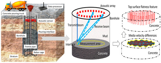
Figure 1.
Schematic diagram of top measurement principle.
Assuming that the borehole of the cast-in-place pile is a standard cylinder, the concrete below the cylinder is poured, and the concrete is solid. Above the cylinder is mud, which is in liquid form. The top surface of the cast-in-place bored pile is the pouring interface between concrete and slurry. To obtain the distance between the top surface of the concrete and the borehole opening, a sound wave array containing multiple sound wave transducers is installed at the borehole opening. Acoustic transducers transmit and receive signals in an orderly cycle, achieving signal acquisition of the entire state of acoustic signals in mud, measurement areas (the pouring interface between mud and concrete), concrete, and the borehole bottom. By utilizing the total waveform reflection method to achieve precise measurement of the top surface position of the cast-in-place bored piles, the 3D morphological feature reconstruction of the top surface elevation of the cast-in-place bored piles is achieved. Subsequently, the flatness information of the top surface of the bored pile is calculated using the elevation information of the top surface of the bored pile, and the quality of the bored pile top is quickly evaluated through the flatness value. The sound waves emitted by the sound wave array (annular arrangement of borehole) propagate through the mud to the concrete mud interface, and the protrusion or depression of the interface will change the length of the sound wave propagation path. In the raised area, the propagation distance of sound waves is shortened, the arrival time of reflected echoes is advanced, and the waveform amplitude is slightly enhanced due to changes in the normal direction of the interface. In the concave area, the propagation distance of sound waves is extended, the arrival time of reflected echoes is delayed, and the amplitude may be slightly attenuated due to scattering. Full waveform inversion can reconstruct the instantaneous shape of the interface, including details such as protrusions and depressions, by analyzing the travel time, amplitude, and frequency changes in echoes at different positions, achieving real-time monitoring of the dynamic changes in the interface during the pouring process.
2.2. Full Waveform Inversion of Top Reflection Echo
The basic principle of the full waveform inversion algorithm is to establish a functional mapping relationship between the residuals between the actual measurement data and the synthesized data of the wave equation, and between the residuals of the actual model parameters and the initial model parameters, gradually correcting the initial model. When the residuals between the actual measurement data and the synthesized data reach a minimum value, the model parameter information of the structure can be obtained. The schematic diagram of the top reflection echo is shown in Figure 2. The full waveform inversion algorithm consists of two parts: the forward process of solving the wave equation to generate synthetic data, and the inversion process of calculating the gradient of the residual function and updating the model with appropriate optimization methods.
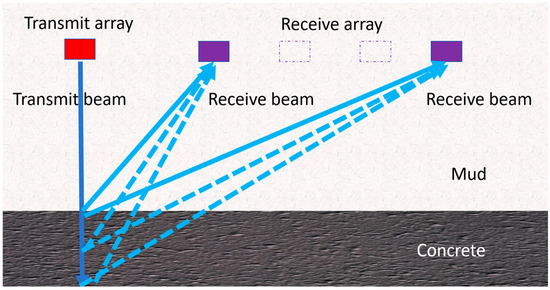
Figure 2.
Schematic diagram of top reflection echo.
The full waveform inversion method of the top reflection echo in this article first provides an initial model containing the conventional sound velocity of two media, mud and concrete. Through forward simulation, the propagation wave field of mud and concrete in the borehole is obtained. The simulation results are compared with the data collected on-site. If the error between the simulation results and the on-site collection results does not meet the given error range, the model is corrected and the above operation is repeated until the error meets the set requirements. Due to the high content of aggregates inside the newly poured concrete and its fast solidification rate, in order to simplify the model, this article considers the newly poured concrete as a solid medium and the slurry above the concrete pouring interface as a fluid medium. Therefore, the method proposed in this article is not only applicable for monitoring the concrete pouring interface during the pouring process, but also for quality inspection of the top of perforated cast-in-place piles.
Due to the fact that the mud in the upper part of the borehole belongs to the fluid medium, while the concrete in the lower part belongs to the solid medium, the full waveform inversion in this paper mainly combines the analysis based on the acoustic elastic wave coupling equation. Due to the viscous effect of concrete in solid media, sound waves tend to exhibit strong frequency dissipation characteristics. However, conventional full waveform inversion based on the acoustic elastic wave coupling equation fails to consider this. Therefore, this paper introduces the relationship between pressure components and normal stress into the viscoelastic wave equation, constructs the acoustic viscoelastic wave coupling equation, and achieves multi parameter full waveform inversion of the acoustic viscoelastic wave coupling equation. The pressure component of the elastic wave field can be calculated by taking the average of the negative normal stress component. By substituting this relationship into the first-order velocity stress viscoelastic equation, the acoustic viscoelastic wave coupling equation for 2D isotropic media can be obtained:
In the formula, represents density. represents time. and represent the horizontal and vertical components of the vibration velocity, respectively. τxx, τzz, and τxz, respectively, represent the normal stress in the x direction, the normal stress in the z direction, and the shear stress component. Full waveform inversion is a method that uses the difference between the collected sound wave signal and the simulated sound wave signal as a constraint, and iteratively updates the model data through optimization algorithms to minimize the difference between the collected data and the simulated data. The objective function in the least squares sense can be expressed as follows:
In the formula, dsyn represents the simulated acoustic data obtained. dobs represents data collected on-site. T is the length of the full waveform acoustic signal. m represents model data. Ω represents the boundary of the model. S(m) represents the objective function to be optimized. According to the principle of the adjoint state method, the partial derivatives of the objective function to be optimized with respect to the Lame coefficients λ and μ can be obtained:
In the formula, represent the difference between the on-site collected data and the simulated acoustic data as disturbance signals, and the backpropagation wavefield obtained through the adjoint state principle corresponds to the adjoint wavefield of , respectively. The gradient formula for longitudinal and transverse wave velocities is as follows:
In the formula, the superscript k represents the k-th iteration. represents the model parameters of the k-th iteration; and represent the longitudinal and transverse wave velocities of the k-th iteration; and represent the Lame coefficients of the k-th iteration. and represent the partial derivatives of the k-th objective function with respect to the Lame coefficients and , respectively. and represent the gradients of longitudinal wave velocity and transverse wave velocity at the k-th iteration, respectively. Based on the calculated gradient, the parameters of the conventional full waveform inversion longitudinal and transverse wave velocity models can be updated, which can be expressed as follows:
In the formula, is the model updated after the k + 1th iteration. is the update step size for the k-th iteration. represents the gradient of the k-th iteration model parameters, which is usually obtained through a line search.
The assumption of treating freshly poured concrete as a solid medium is set in this article, because although the freshly poured concrete is in the process of transforming from a fluid state to a solid state, it already has certain viscoelastic properties in the initial setting stage and is not a completely ideal fluid. At this point, the internal aggregate skeleton of the concrete is initially formed, which can transmit a weak shear stress. Therefore, although the transverse wave decays quickly, it can still be detected (especially in close range propagation scenarios). As a typical fluid, mud has a shear modulus of 0, and transverse waves cannot propagate. In the model, the transverse wave velocity in the mud area is set to 0 to distinguish the type of medium. The core of full waveform inversion is to use complete waveform information (including longitudinal waves, transverse waves, and reflected/refracted waves) to improve the accuracy of model parameters. Even if the transverse wave signal in concrete is weak, incorporating the transverse wave velocity parameter can constrain the coupling problem between longitudinal wave velocity and density during the inversion process, reducing ambiguity. In this article, the transverse wave velocity is inverted through gradient calculation (Equation (4)). In actual calculations, the transverse wave weight is dynamically adjusted according to the medium type (concrete/mud) to ensure that the transverse wave parameters in the fluid region do not affect the final result.
2.3. Calculation of the Flatness of the Top of the Cast-in-Place Bored Pile
A pile top grid index matrix is established in order of radius and angle, using a 2D sequential grid index (i, j). I represents the i-th scanning circle around the center point of the pile top grid, j represents the j-th scanning line around the center point of the pile top grid, and the 2D sequential grid index is shown in Figure 3a. Establish a 3D Cartesian coordinate system with the plane position of the 2D sequential grid index (0, 0) as the coordinate origin, as shown in Figure 3b. The calculation expression for any point (X, Y, Z) on the top surface of the cast-in-place bored pile is as follows:
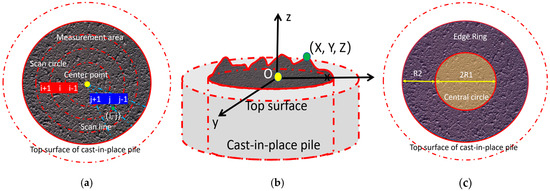
Figure 3.
Schematic diagram of different areas at the top position. (a) 2D sequential grid index, (b) 3D Cartesian coordinate system, and (c) center position partition.
Among the variables, R represents the radius of the measurement area. P represents the total number of scanning circles included in the measurement area. Q represents the total number of scanning lines included in the measurement area. hz represents the elevation of the point relative to the plane where the grid index (0, 0) is located.
When obtaining 3D data samples of the top surface of the cast-in-place pile, random sampling is performed on the dataset obtained from the grid index. Due to the fact that a plane requires at least three non collinear points to be determined, and the plane used for fitting in this article is the pile top design reference plane (horizontal plane), whose elevation is determined based on the pile top design elevation, three data points were selected for the random sampling sample set. One horizontal reference plane is fitted using three randomly sampled points as a reference for evaluating the flatness of the pile top; for the analysis of the flatness of different areas on the pile top, the distance and deviation of each point are calculated based on the unified horizontal reference plane to ensure the consistency of the evaluation criteria. The plane equation determined by these three points is the benchmark plane equation used to evaluate the flatness of the pile top, as follows:
Among the variables, z is the vertical coordinate of a point on the top surface of the cast-in-place bored pile in 3D space. A and B are the coefficients of the first-order term of the plane equation. x is the horizontal coordinate of a point on the top surface of the cast-in-place bored pile in 3D space. y is the vertical coordinate of a point on the top surface of the cast-in-place bored pile in 3D space. C is the constant term of the plane equation. Using the cross-sectional data points of the top surface of the cast-in-place bored pile fitted in the above steps, the distance and standard deviation from the sampling point to the plane are calculated, and expressed as follows:
Among the variables, is the distance from the sampling point to the plane. is the average distance from the sampling point to the plane. is the standard deviation between the distances from each point to the plane. After obtaining the standard deviation of a single cross-section sampling point, the values of multiple different vertical cross-sections can be averaged to achieve comprehensive evaluation of the top surface of the cast-in-place bored pile. In practical engineering, an uneven pile top can lead to an uneven stress distribution during the installation of the upper structure, which may cause premature failure, uneven settlement, and overall performance degradation of the structure. Due to the significant influence of the physical structure of the pouring pipe during the pouring process, the unevenness of the center position of the pile top is mainly affected by factors such as pouring speed, borehole wall roughness, and bottom sediment. Therefore, this article proposes the concepts of the center circle and edge ring to achieve a comprehensive evaluation of the elevation between the center position and the outer position of the cast-in-place bored pile top, and to realize a pile top quality detection method that comprehensively considers the differential characteristics between the center and edge positions of the pile top.
The difference in flatness between the center and periphery of the pouring interface of the borehole pile is a barometer of the construction process (such as fabric, vibration, and concrete performance). Mastering its characteristics can achieve quality pre control, process optimization, and structural safety assessment. Meanwhile, this difference is directly related to construction defects (segregation, insufficient vibration), flow problems (abnormal fluidity), and structural risks (stress concentration, reduced durability), and is one of the core monitoring indicators for borehole pile engineering quality control. In order to achieve a comprehensive analysis of the flatness of the center and edge positions of the pile top, the measurement area is divided into center positions, as shown in Figure 3c. Define the area near the center as the center circle, and the circular ring around the center periphery as the edge ring. If the radius of the central circle is R1 and the radial width of the edge ring is R2, then R1 + R2 = R. Define the pile top flatness factor PD as follows:
Among the variables, is the distance value from the sampling point (i, j) to the plane. is the standard deviation between the sampling point (i, j) and the plane distance. and are the weighting coefficients of the elevation distance value and standard deviation, respectively. If there is not much difference in the acoustic data obtained for the flatness of the center and periphery of the pile top interface, then the values of and are each 0.5. If the sound wave data obtained from the center of the pile top interface is better than the sound wave data obtained from the periphery of the pile top interface, then the value of should be greater than 0.5, and its specific degree needs to be selected based on the actual situation. If the sound wave data obtained from the center of the pile top interface is worse than the sound wave data obtained from the periphery of the pile top interface, then the value of is greater than 0.5, and its specific degree needs to be selected based on the actual situation. From Equation (9), it can be seen that when the flatness factor PD of the pile top is equal to 1, it indicates that the flatness of the center position and the outer position of the pile top are relatively close, that is, the fluctuation is not significant. When the flatness factor PD of the pile top is less than 1, it indicates that the flatness of the center position of the pile top is higher than that of the outer position, that is, the fluctuation in the outer position is greater. When the flatness factor PD of the pile top is greater than 1, it indicates that the flatness of the center position of the pile top is lower than that of the outer position, that is, the fluctuation in the center position is greater. The pile top flatness factor PD proposed in this article is a comprehensive index obtained by integrating the distance values and standard deviations of each sampling point in the center circle and edge ring area of the pile top to the fitting reference plane, and weighting them to quantify the flatness difference between the two. When PD = 1, it indicates that the flatness of the center and periphery is close and the overall undulation is uniform. When PD < 1, it indicates that the flatness of the center is better than that of the periphery, and the undulation of the periphery is greater. When PD > 1, it reflects that the flatness of the periphery is better than that of the center, and the fluctuation in the center is more obvious. This factor takes into account both the elevation difference and the uniformity of undulations, and can intuitively reflect the uniformity of pile top pouring, providing a basis for quickly judging construction quality (such as material distribution and vibration issues).
2.4. Experimental Analysis
In order to verify the feasibility and correctness of the method proposed in this article, relevant experimental analysis is conducted indoors. The test container uses a stainless-steel drum to simulate the cast-in-place bored pile borehole. The diameter of the stainless-steel drum is 800 mm, and the height is 1100 mm. The test container is filled with a 10% sodium-based bentonite liquid test medium, with a height of 400 mm. C30 concrete is poured at the bottom of the drum to simulate the pile body, with a height of about 200 mm. The acoustic array probe has 96 elements, and the outer diameter of the disc of the acoustic array probe is 360 mm. The elements are evenly distributed in a circular shape (with a spacing of 7.5 mm), supporting 0–360° omnidirectional scanning. The data acquisition system includes a signal controller (output voltage 0–100 V, adjustable frequency), a signal collector (sampling rate 10 MHz, resolution 16 bit), a computer, and self-developed data processing software, which are used to control the timing of sound wave transmission/reception, store raw waveform data, and call the full waveform inversion algorithm. The experiment in this article simulates the scenario of “pile top quality inspection during the pouring process of cast-in-place piles”, so the C30 concrete poured in the bucket is in an uncured state to simulate the actual pile top shape inspection requirements during the pouring process of cast-in-place piles. The data processing software developed independently in this article is based on Python 2.6 language and combined with Matplotlib 1.5 library to achieve result visualization.
The schematic diagram of the experimental device is shown in Figure 4. The purpose of this experiment is to achieve three core objectives: (1) Verify the accuracy of the full waveform inversion method for measuring pile top elevation and evaluate its measurement accuracy in simulated drilling environments by comparing the inversion results with the actual pile top elevation. (2) Verify the reliability of the calculation method for pile top flatness (flatness factor PD) and analyze its ability to distinguish different pile top shapes (flatness, central protrusion, edge depression, etc.). (3) Explore the influence of medium characteristics (such as mud concentration) on measurement results and verify the stability of the method under different operating conditions.
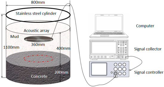
Figure 4.
Schematic diagram of experimental apparatus.
The sound wave array works in a “circular scanning and layer by layer progressive” mode: scanning 360° from the center to the outside, collecting echo signals every 1° interval, and obtaining a total of 10 scanning data cycles (corresponding to grid indices i = 0 to i = 9). By conducting detailed cyclic full waveform data acquisition on each of the 48 array elements, it is ensured that the waveform data of each element are recorded completely and accurately. Subsequently, all collected waveform data are filtered (50–200 kHz bandpass filtering) and denoised (wavelet threshold denoising), and then inputted into the full waveform inversion algorithm in Section 2.2 of this article (initial model sound velocity: mud 1500 m/s, concrete 3500 m/s. After 50 iterations with a step size determined by a line search, the sound velocity distribution images of different media inside the stainless-steel barrel are inverted, as shown in Figure 5.
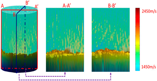
Figure 5.
Distribution of sound velocity differences.
The different colors in Figure 5 represent different values of sound velocity, showing the distribution of sound wave propagation velocity in different media. From Figure 5, it can be clearly observed the variation in the sound velocity of the medium above the concrete. The sound velocity in the mud area is relatively low and there is a certain velocity gradient, which may be related to the uneven concentration distribution of the mud. The sound velocity in the concrete area is relatively high, which can distinguish the boundary between the mud area and the top of the concrete, as well as the sound velocity distribution characteristics inside the concrete. Furthermore, the sound velocity distribution data of the concrete top surface are extracted from the inversion results, and the 3D shape of the pile top is reconstructed based on the correspondence between sound velocity and elevation (the interface position corresponding to the sound velocity mutation), combined with the grid index and 3D coordinate transformation method in Section 2.3. In order to verify the accuracy of the full waveform inversion method in the pile top elevation measurement, this paper conducts a comparative study between the reconstructed pile top shape and the actual poured pile top shape. The actual image of the poured pile top is shown in Figure 6a. By using a pseudo color map to represent the relative distance of elevation, the top view result is shown in Figure 6b. From the comparison between Figure 6a,b, it can be seen that the reconstructed pile top shape is consistent with the actual pile top shape in terms of overall trend, especially in the fluctuation changes between the center and edge positions of the pile top, which have a high similarity.
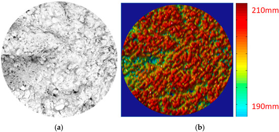
Figure 6.
Comparison of top surface morphological features. (a) Pile top image; (b) inverted top view.
In order to more intuitively observe the fluctuation in the elevation of the concrete top surface, the concrete top surface is divided into four sections for analysis, as shown in Figure 7a. It includes four profiles: a-a’, b-b’, c-c’, d-d’. The elevations corresponding to the four sections of concrete are shown in Figure 7b. From Figure 7b, it can be seen that the elevation of the concrete top surface is mainly concentrated between 195 and 205 mm. The fluctuation in the a-a’ section is the largest, and the fluctuation in the c-c’ section is the smallest. This result is basically consistent with the actual distribution of the fluctuation in the concrete pile top, which verifies the feasibility of the method proposed in this paper.
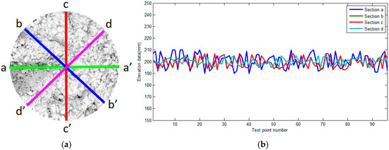
Figure 7.
Comparison of elevation of different profiles on the top surface. (a) Schematic diagram of section division; (b) different section elevations.
In addition, to further verify the effectiveness of the full waveform inversion method in pile top elevation measurement, a laser rangefinder was used to scan the actual elevation of the pile top surface as the true value dataset. The high-precision laser rangefinder (accuracy ± 0.1 mm) is used as the true value measurement tool. The laser point cloud data are compared with the horizontal (a-a’ section) elevation data obtained in this article; the results are shown in Figure 8a, and the relative error is shown in Figure 8b. The the laser point cloud data are compared with the vertical (c-c’ section) elevation data obtained in this article; the results are shown in Figure 8c, and the relative error is shown in Figure 8d.
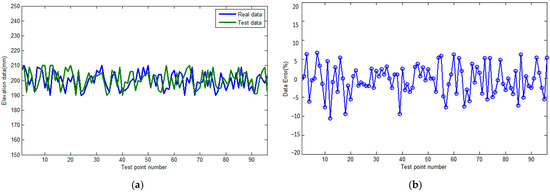
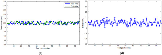
Figure 8.
Comparison of point cloud data results. (a) Comparison of horizontal direction. (b) Relative error in horizontal direction. (c) Comparison of vertical direction. (d) Relative error in vertical direction.
From the data and trends shown in Figure 7, it can be seen that the concrete elevation values obtained in this article are relatively close to the true values, with an error of no more than 10% in the horizontal direction and no more than 5% in the vertical direction. This is mainly due to the fact that the test object has greater fluctuations in the horizontal direction and smaller fluctuations in the vertical direction. Due to the fact that this article mainly relies on the elevation data obtained from full waveform inversion, the inversion results are highly dependent on the number of sensors. Under the same number of sensor configurations, if the terrain undulation is relatively low, the elevation data inverted by these sensors will be more accurate and reliable. This is because the low undulating terrain reduces signal interference and error accumulation, allowing sensors to more accurately capture and analyze terrain information. On the contrary, under the same number of sensor configurations, when the terrain undulation is severe, the inverted elevation data will show relatively large errors. This is because severe fluctuations increase the complexity and uncertainty of signal propagation, leading to more errors in sensor data acquisition and processing, thereby affecting the accuracy and precision of elevation data. Therefore, the degree of terrain undulation has a significant impact on the accuracy of elevation data inversion.
In order to quantitatively evaluate the accuracy of reconstructing the shape of the pile top, the sound velocity distribution data obtained from inversion is used, combined with the calculation method for the flatness of the pile top of the cast-in-place bored pile proposed in Section 2.3 of this paper. The flatness factor PD of the pile top can be calculated, and then the flatness of the pile top can be quantitatively evaluated. Before conducting the leveling of the pile top, it is necessary to divide the measurement area into central positions. In order to analyze the differential characteristics of evaluation results corresponding to different center circle and edge ring sizes, the top surface of the concrete is divided into three different circular ring regions (l-ring, m-ring, n-ring). The size corresponding to the l ring is two-thirds of the measurement area size, which corresponds to a diameter of 240 mm. The size corresponding to the m ring is one-half of the measurement area size, which corresponds to a diameter of 180 mm. The size corresponding to the n ring is one-third of the measurement area size, which corresponds to a diameter of 120 mm. The center position of the concrete top surface is divided as shown in Figure 9a, that is, the concrete top surface is divided into two-thirds, one-half, and one-third, respectively. Flatness analysis is conducted on the areas enclosed by the l-ring, m-ring, and n-ring, as shown in Figure 9b. In Figure 9b, when the top surface of the concrete is divided into two-thirds, the central circle is the circular area inside the l circle, and the edge ring is the circular area outside the l circle. When dividing the top surface of concrete into one-half, the central circle is the circular area inside the m circle, and the edge ring is the circular area outside the m circle. When dividing the top surface of concrete into one-third, the central circle is the circular area on the inner side of n circles, and the edge ring is the circular area on the outer side of n circles.
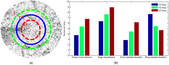
Figure 9.
Comparison of differences in flatness characteristics. (a) Center position division. (b) Flat characteristic distribution.
From Figure 9, it can be seen that when the division size of the concrete top surface is two-thirds of the measurement area size, the average distance between the center circle and the edge ring is the highest. When the division size of the concrete top surface is one-third of the measurement area size, the average distance between the center circle and the edge ring is the smallest. When the division size of the concrete top surface is two-thirds of the measurement area size, the standard deviation of the center circle is the largest and the standard deviation of the edge ring is the smallest. When the division size of the concrete top surface is one-third of the measurement area size, the standard deviation of the center circle is the smallest and the standard deviation of the edge ring is the largest. The selection of measurement area size has a significant impact on the evaluation of the center circle and edge ring. In addition, the calculation using only the average distance as the pile top flatness factor will be represented by MD. The calculation using only the standard deviation as the pile top flatness factor will be represented as SD. The calculation of the pile top flatness factor using both the distance mean and standard deviation in this article is represented by PD. The analysis of the flatness of the concrete top surface in the measurement areas of one-third, one-half, and two-thirds in sizes is shown in Figure 10.
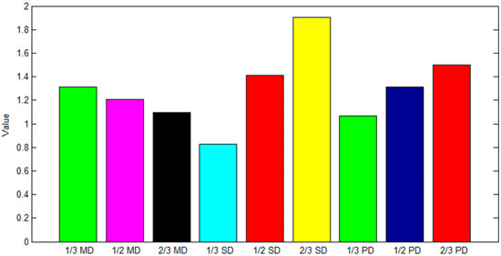
Figure 10.
Top surface flatness comparison of measurement area.
From Figure 10, it can be seen that when using measurement areas of different sizes to analyze the flatness of the concrete top surface, the evaluation results using the pile top flatness factor PD proposed in this paper are more comprehensive and accurate. Specifically, there are significant differences in the flatness factors calculated by MD, SD, and PD methods in the measurement areas of one-third and two-thirds in sizes. In the measurement area of one-half in size, the flatness factors calculated by MD, SD, and PD methods are relatively close, and the overall fluctuation is small. Simply analyzing the flatness from the perspective of the average distance, the flatness factor is greater in the measurement area of one-third in size, indicating a significant difference in the distance between the center circle and the edge ring. The flatness factor is smaller in the measurement area of two-thirds in size, indicating that the distance difference between the center circle and the edge ring is small. Simply analyzing the flatness from the perspective of standard deviation, the flatness factor is smaller in the measurement area of one-third in size, indicating that the distance between the center circle and the edge ring fluctuates less. The flatness factor is relatively large in the measurement area of two-thirds in size, indicating that the distance between the center circle and the edge ring fluctuates greatly. This article comprehensively utilizes the average distance and standard deviation as the flatness factor of the pile top, which can take into account the elevation value and fluctuation difference of the concrete top surface, thus providing more reliable data support for the quality analysis of the top surface. In addition, there are significant differences in the evaluation of pile top flatness under different measurement areas of different sizes. Therefore, in practical engineering applications, it is necessary to comprehensively evaluate the size division of the measurement area.
In summary, the proposed method for detecting the top of bored piles based on full waveform inversion not only achieves accurate measurement of pile top elevation, but also quantifies the evaluation of pile top flatness by introducing the pile top flatness factor PD. This method has the advantages of easy operation, accurate measurement, and strong applicability, providing a new technical means for rapid prediction and comprehensive evaluation of the quality of the top of drilled cast-in-place bored piles. However, the method proposed in this article also has limitations, as it mainly relies on the elevation data obtained from full waveform inversion, and its inversion results are highly dependent on the number of sensors. When the complexity of the test object is high and the number of sensors is the same, the lower the fluctuation is, the more accurate the inverted elevation data will be. When the complexity of the test object is high and the number of sensors is the same, the greater the fluctuation, the greater the relative error of the inverted elevation data. Although increasing the number of sensors can improve the accuracy of concrete elevation measurement to some extent, it will incur more material and computational costs. Therefore, when adopting the method proposed in this article, it is necessary to comprehensively evaluate the measurement requirements and usage costs.
3. Conclusions
In response to the technical difficulty of real-time monitoring and accurate evaluation of the interface morphology of the pile top in the traditional concrete pouring process, this paper proposes a method for detecting cast-in-place bored pile top surfaces based on full waveform inversion. Firstly, based on fully considering the frequency dissipation characteristics of sound waves propagating in concrete and mud, a coupling equation between sound waves and viscoelastic waves is constructed, achieving full waveform inversion of multiple parameters of concrete and mud in the borehole, providing a solid data foundation for subsequent analysis of pile top morphology. Subsequently, in order to more accurately distinguish the differential characteristics between the center circular area and the edge circular area of the pile top, this paper innovatively proposes the pile top flatness factor and constructs a comprehensive evaluation method for the elevation between the center position and the center peripheral position of the cast-in-place bored pile top, which can comprehensively and meticulously evaluate the shape of the pile top. Finally, in order to verify the feasibility and accuracy of the proposed method, detailed indoor experiments are conducted. The experimental results show that the detection method proposed in this article can not only accurately reflect the actual elevation of the pile top, ensuring the accuracy of the measurement data, but also effectively distinguish different forms of the pile top and reveal their subtle differences. In terms of measuring pile top elevation and evaluating pile top flatness, this method demonstrates high accuracy and reliability, significantly improving detection efficiency and accuracy. This research achievement provides strong technical support for the rapid prediction of pile top quality, which is expected to be widely applied in practical engineering, further improving the quality and management level of concrete pouring.
Author Contributions
Writing—original draft preparation, M.C. and J.W.; writing—review and editing, J.Z. and H.H.; Resources, L.W., H.Z. and H.L.; funding acquisition, M.C.; methodology, J.W.; project administration, J.Z., H.H., L.W., L.W., H.Z. and H.L. All authors have read and agreed to the published version of the manuscript.
Funding
This research was funded by the Open Foundation of Science and Technology Innovation Center of Hubei Institute of Urban Geological Engineering (No. KCJJ202401), and the Key R&D Plan Project in Hubei Province (No. 2023BAB099).
Institutional Review Board Statement
Not applicable.
Informed Consent Statement
Not applicable.
Data Availability Statement
All data, models, and code generated or used during this study appear in the submitted article.
Acknowledgments
All the images and data are from our actual tests and permitted by the owners. We are compliant with ethical standards, and all authors declare that this paper has no conflicts of interest. Finally, we are grateful for the many helpful and constructive comments from many anonymous reviewers.
Conflicts of Interest
Authors Ming Chen, Jiwen Zeng, Hao He and Lu Wang were employed by the company Wuhan Geological Survey Engineering Co., Ltd. Author Haicheng Zhou was employed by the company Xiong’an New Area Construction Engineering Quality and Safety Testing Service Center. Author Houcheng Liu was employed by the company Wuhan Zhongke Kechuang Engineering Testing Co., Ltd. The remaining author declares that the research was conducted in the absence of any commercial or financial relationships that could be construed as a potential conflict of interest.
References
- Wang, J.; Liu, H. Defect detection method of underwater bored cast in place bored pile based on optical image in borehole. J. Civ. Struct. Health Monit. 2023, 14, 189–207. [Google Scholar] [CrossRef]
- Wang, J.; Xu, H.; Wang, B.; Zou, J.; Liu, H. Accurate detection technology of super long bored cast in place bored pile concrete pouring thickness based on ultrasonic inclined plane reflection measurement. Measurement 2022, 198, 111314. [Google Scholar] [CrossRef]
- Wang, J.; Liu, H.; Han, Z.; Hu, S.; Tang, D.; Chen, M. Research on the detection method of pouring interface for ultra deep bored pile based on total pulse reflection. China Test. 2025, 51, 133–142. [Google Scholar]
- Feng, Z.; Xu, B.; Chen, H.; Xia, C.; Cai, J. Study on the Influence of Different Cave Treatment Measures on the Bearing Characteristics of Pile Foundations. J. Build. Sci. Eng. 2024, 41, 151–158. [Google Scholar]
- Bo, Q.; Li, C.; Shang, W.; Gao, C.; Liu, J. Research on the Impact of Offshore Hammer Sinking Pile Process on Existing Approach Bridges. J. Transp. Sci. Eng. 2025, 41, 86–96. [Google Scholar]
- Wang, B.; Zhou, D.; Han, X.; Zhao, J.; Cao, Y.; Wang, S. Analysis of the Impact of Tunnel Adjacent Pile Foundation Construction Based on HSS Model. J. Build. Sci. Eng. 2023, 40, 160–171. [Google Scholar]
- Xu, B.; Yin, B.; Yang, G.; Shi, W.; Liu, L. Analysis of vertical bearing characteristics of the cast in place bored piles considering the influence of changes in soil parameters on pile side. Sichuan Build. Sci. Res. 2024, 50, 40–47. [Google Scholar]
- Xing, K.; Wu, W.; Zhang, K.; Liu, H. Analysis Method for Horizontal Bearing Capacity of Large Diameter Pile Foundations Based on Improved Strain Wedge Model. Saf. Environ. Eng. 2020, 27, 8. [Google Scholar]
- Wang, S.; Duan, W.; Ma, C.; Zhang, T. Analysis of horizontal bearing capacity of pile foundation based on in-situ testing technology in geotechnical engineering. Saf. Environ. Eng. 2018, 25, 8. [Google Scholar]
- Sun, H.; Li, W.; Zhang, Z.; Liu, T.; Wang, Y.; Liu, T.; Liu, H. Research on Geological Information Evaluation of Underground Rock and Soil Engineering Based on Multi Attribute Testing in Holes. Saf. Environ. Eng. 2023, 30, 62–69. [Google Scholar]
- Zhou, Q.; Luo, F.; Chai, B.; Zhou, A. Comparative study on machine learning algorithms for predicting ground temperature in deep buried long tunnels. Saf. Environ. Eng. 2025, 32, 137–147. [Google Scholar]
- Zhang, G.; Jiang, J.; Lv, G.; Hu, J.; Xiong, F.; Liao, Y.; Zheng, H.; Li, Q. Automatic generation algorithm for rock core RQD based on object detection and image segmentation. Saf. Environ. Eng. 2025, 32, 100–106. [Google Scholar]
- Liu, Y.; Zheng, H.; Feng, L. Time domain simulation of 3D sound wave scattering. J. Ningxia Univ. Nat. Sci. Ed. 2011, 32, 5. [Google Scholar]
- Hua, J.; Cai, Y.; Lian, X.; Qian, L.; Cai, W.; Tang, B.; Sun, Z. Research on the Quality Evaluation Method of Pottery Ore Based on TIMA Testing. East China Geol. 2024, 45, 488–497. [Google Scholar]
- Jokūbaitis, A.; Skuodis, Š.; Šneideris, A.; Zavalis, R. Application of non-destructive methods for bored concrete piles installed 34 years ago. Case Stud. Constr. Mater. 2024, 20, e03104. [Google Scholar] [CrossRef]
- Rybak, J.; Schabowicz, K. Acoustic wave velocity tests in newly constructed concrete piles. In Proceedings of the NDE for Safety: 40th International Conference and NDT Exhibition 2010, Pilsen, Czech Republic, 10–12 November 2010; pp. 247–254. [Google Scholar]
- Qiu, H.; He, H.; Ayasrah, M.; Huang, W. Application Study of the High-Strain Direct Dynamic Testing Method. Appl. Sci. 2024, 14, 6714. [Google Scholar] [CrossRef]
- Liu, L.; Shi, Z.; Tsoflias, G.P.; Peng, M.; Liu, C.; Tao, F.; Liu, C. Detection of Karst Cavity Beneath Cast-in-place Pile Using Instantaneous Phase Difference of Two Receiver Recordings. Geophysics 2020, 86, EN27–EN38. [Google Scholar] [CrossRef]
- Onder Cetin, K.; Cuceoglu, F.; Ayhan, B.U.; Yildirim, S.; Aydin, S.; Demirdogen, S.; Er, Y.; Gurbuz, A.; Moss, R.E.S. Performance of hydraulic structures during 6 February 2023 Kahramanmara, Türkiye, earthquake sequence. Earthq. Spectra 2024, 40, 2231–2267. [Google Scholar] [CrossRef]
- Gabrielaitis, L.; Papinigis, V.; Sirvydaitė, J. Assessment of different methods for designing bored piles. Eng. Struct. Technol. 2012, 4, 7–15. [Google Scholar] [CrossRef]
- He, X.; Chen, H.; Wang, X. Ultrasonic leaky flexural waves in multilayered media: Cement bond detection for cased wellbores. Geophysics 2014, 79, A7–A11. [Google Scholar] [CrossRef]
- Liang, X.; Xu, P.; Bai, X.; Li, Z.; Sun, R.; Nie, T. Exploration on the initial model construction of full waveform inversion in Jinggong Coal Mine. China Coal 2024, 50, 90–100. [Google Scholar]
- Wang, Z.; Deng, J.; Chen, H.; Yin, M.; Feng, M. Analysis of Transient Electromagnetic Full Time Response Characteristics of Full Waveform Loop Source Well. Resour. Environ. Eng. 2024, 38, 323–330. [Google Scholar]
- Li, Z.; Du, S.; Guo, M.; Xu, J. Intelligent coal mine transparent geological new technology—Research and practice of mine seismic full waveform inversion technology. Intell. Min. 2023, 4, 54–62. [Google Scholar]
- Liu, G.; Mao, S.; Song, P.; Tan, J.; Zhao, B.; Jiang, X. Multi parameter full waveform inversion based on acoustic viscoelastic wave fluid structure coupling equation. Pet. Geophys. Explor. 2025, 60, 700–709. [Google Scholar]
Disclaimer/Publisher’s Note: The statements, opinions and data contained in all publications are solely those of the individual author(s) and contributor(s) and not of MDPI and/or the editor(s). MDPI and/or the editor(s) disclaim responsibility for any injury to people or property resulting from any ideas, methods, instructions or products referred to in the content. |
© 2025 by the authors. Licensee MDPI, Basel, Switzerland. This article is an open access article distributed under the terms and conditions of the Creative Commons Attribution (CC BY) license (https://creativecommons.org/licenses/by/4.0/).