Article

Comparison between Predicted and Measured Moisture Content and Climate in 12 Monitored Timber Structures in Switzerland

Institute for Architecture, Timber Construction and Structures, Bern University of Applied Sciences, 2504 Biel/Bienne, Switzerland
*
Author to whom correspondence should be addressed.
Buildings 2021, 11(5), 181; https://doi.org/10.3390/buildings11050181
Submission received: 2 March 2021 / Revised: 20 April 2021 / Accepted: 22 April 2021 / Published: 24 April 2021
(This article belongs to the Special Issue Timber Structures: Latest Developments, Challenges, and Perspectives)

Abstract

:
Wood is a hygroscopic material that primarily adapts its moisture content to the surrounding relative humidity. The climate in a structure or building depends on the building type and the region the structure is located in. In this study, the effect of region on the moisture content of wood was investigated. Measurements taken in 12 ventilated timber structures were compared to the theoretical equilibrium moisture content calculated from the relative humidity and temperature in 107 meteorological stations across Switzerland. The monitored load-bearing elements were made of softwood and protected from the direct impact of weather. The climatic conditions around the Alps, a mountain range that runs from France to Austria and crosses Switzerland, can be divided into the following three different regions: (1) south of the Alps, where the climate is affected mainly by the Mediterranean sea; (2) north of the Alps, where the climate is affected by the Atlantic Ocean; and (3) the inner Alps, where the climate is considered to be relatively dry. The climatic conditions of the three separate regions were reflected in the measurements made in the monitored timber structures. Differences between the regions were quantified. The moisture content and relative humidity, similarly to temperature, depended on altitude (above sea level).

Graphical Abstract

1. Introduction

Wood is a hygroscopic material that experiences moisture content (MC, expressed as mass percentage (M%)) changes during its service life due to climate changes in buildings [1]. The MC of wood primarily depends on its surrounding climate and engineers need to anticipate the climatic conditions a structure will experience. The climate in a building is of interest as it defines the strength and stiffness of the load-bearing elements of a structure [2,3]. The climate in a building is not only affected by the building type and building envelope, but also by climate conditions outside of the building.
The Swiss climate is characterized by three main local climate conditions due to the presence of the Alps [4]. For instance, the inner Alps are known to be dryer due to rain shadowing [5,6] than the densely populated Central Plateau, but to what extent this can or needs to be accounted for is not known. The tradition of timber construction has been strong throughout the centuries and, therefore, different examples of the longevity of timber can be found in buildings and bridges. Structural protection by either building a roof with a large overhang or cladding load-bearing timber elements is the favored building practice. Materials, areas of application, and performance requirements, however, continuously develop in modern architecture. Thus, more and more timber structures are also being built high in the mountains. Timber is a popular building material as it is abundantly available and allows for short construction times. Light, prefabricated elements can be flown to a construction site if access by road is difficult.
Structural engineers need to know how load-bearing elements of a structure will respond (MC) to the climatic conditions where it is installed. MC in load-bearing elements is accounted for through the system of Service Classes found in Eurocode 5 (EN 1995) [2]. The Swiss standard mentions that MC in the pre-Alpine region (north side) and the Jura are higher. In the inner Alps region, MC has been found to be lower than in the Central Plateau; for both regions, however, absolute values are not mentioned [3]. Moisture conditions—i.e., either too moist, too dry, or varying—accounted for half of the observed structural damage in evaluated large-span timber structures located in southern Germany. The observed damages included, for instance, cracks perpendicular to the grain [7,8].
One study monitored the indoor climate and MC of load-bearing beams in 21 buildings in southern Bavaria, Germany [9]. The considered building types in this study were three swimming pools, four ice rinks, three horseback riding halls, three sports halls, two production halls, three livestock halls, and three storage halls. Another study extended the results by considering the climate and MC in three cable car stations and three bridges [1]. These two studies help in defining the expected MC for different building types, i.e., how dry or how moist a structure is. To avoid fungal attacks, the MC in load-bearing elements is recommended to be maintained below 20 M%. This criterium is usually met in large-span structures [1,9], but is critical in ice rinks and agricultural buildings [10]. If it is higher, the risk of fungal attack is still small if the temperature (T) remains low [11].
In this study, the regional conditions of built timber structures were analyzed. Monitoring data obtained from 12 different buildings across Switzerland were compared to the climate measured in 107 meteorological stations across the country. The available monitoring data allowed for a comparison of the meteorological data with measurements of the following continuously monitored timber structures: (1) ice rinks and horse-riding halls where the relative humidity (RH) was over 90% (e.g., MC > 20 M%) for several months during the year; (2) cable car stations located in the Alps at over 1500 meters above sea level (m.a.s.l.); and (3) bridges. The monitored load-bearing elements were made of softwood (Norway spruce and pine) and resembled Service Class 2 conditions according to Eurocode 5 (EN 1995) [2]. The monitored elements were neither coated nor exposed to rain or sun.

2. State of the Art

2.1. Alpine Climate

In the inner Alps (Figure 1), dry climates and sub-freezing temperatures dominate in winter. The climate in the Central Plateau, which is at an altitude of 400 to 500 m above sea level and is densely populated, is mild and affected by weather from the westerly and northerly direction; it is also a region that is known for being overcast (clouds) in the autumn and winter. The high mountains running from east to west act as a climate and rain barrier [4,5], leading to large variations in the durability of exposed wood [12]. The altitude of the mountains causes differences in climate types; the south is affected more by the Mediterranean Sea and experiences milder winters [4]. Figure 1 shows the locations of the 12 monitored structures and 107 meteorological stations used to compare the predicted and measured climate and MCs.

2.2. Methods for Relating Climate to Region

The Köppen and Geiger maps [6,13,14] and biogeographical regions [15,16] offer a classification of climate that depends on the topography, temperature, precipitation, and vegetation. General applications of the Geiger and Köppen maps can be found in studies of river discharge, vegetation coverage, human thermal comfort by urban street configurations, air pollution, and more [6]. The classification depends on temperature and precipitation [13], but does not consider RH, a dominant factor in wood MC in unexposed wooden components.
The biogeographical regions are defined as areas with similar animal and plant distributions or shared characteristics and are based on experience [17]. The classification separates regions by altitude, water bodies, etc. and offers a classification of region based on typology.
The Scheffer Climate Index (SCI) offers a third possibility for mapping the relationship between climate and region [18]. It is used to model fungal decay in wood and decay hazard mapping and can estimate exposure-related dosage in a quantitative manner [18,19]. Similar to the Geiger and Köppen classification, the SCI is based on T and rainfall.
Figure 2 shows the six main biogeographical regions and 11 smaller regions identified for Switzerland [16]. The six biogeographical regions can be further organized into the following three larger regions using the description given in Section 2.1 [4]:
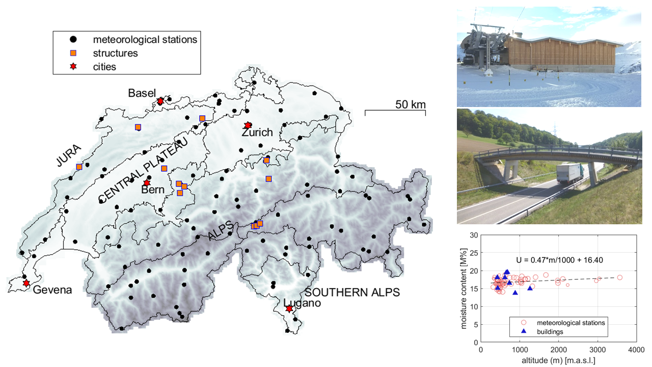
  • North of the Alps (red), i.e., Jura, Central Plateau, the Northern Alps;
  • Inner Alps (blue), i.e., the Western and Eastern Alps;
  • South of the Alps (green), i.e., the Southern Alps.

2.3. Climate and Timber Structures across the European Continent

RH and T data obtained from meteorological stations were used to perform simulations of MC developments and moisture-induced stresses in timber cross-sections [20]. Both MC and moisture-induced stress were greater in northern Europe than in southern Europe.
The Durable Timber Bridges project [21] focused on the durability and further development of timber bridges. Along with measurements of the resistance of timber to decay, maps were set up to indicate areas in Europe where wood was prone to mold and decay [22].
The theoretical equilibrium MC has been calculated for 262 locations in the USA and 122 locations across the globe [23]. In Central Europe, autumn is generally the humid period and spring is the driest. The calculated monthly averages for MC from this study for Geneva, Bern, and Zurich, along with four other cities north and south of the Alps, are listed in Table 1. The MC averages are valid for softwood and based on the Simpson equations (Section 2.6). There was little difference between the cities located in Switzerland, all of which are located in the Central Plateau region (Figure 1 and Figure 2). It can be observed that the two cities south of the Alps experienced less variation in the predicted MC over the year than the two cities north of the Alps.

2.4. Relative Humidity

RH and T are the two main parameters used to calculate predicted MC [24,25] (see also Section 2.5 and Section 2.6). RH can be measured using different methods [24]. The Swiss Federal Office for Meteorology and Climatology measures RH using the following two methods: (1) with a dew-point monitor, where a mirror is cooled to identify the point of condensation (Thygan); (2) with a hygroscopic polymer [26,27]. In the latter, RH is measured directly. In the former, it needs to be calculated from the relationship between the air temperature and dew-point temperature [27] as follows:
H = 100 × exp((a1 × Td)/(a2 + Td) − (a1 × T)/(a2 + T)),
where H is the RH (%), Td is the dew-point temperature (°C), and T is the air temperature (°C). The parameters are a1 = 17.368 and a2 = 238.83 below 0 °C, and a1 = 17.856 and a2 = 245.52 above 0 °C. The difference for RH in subzero temperatures is necessary as the vapor pressure above ice is different from the vapor pressure above supercooled water [28]. Similar relationships, such as the semi-empirical Kirchhoff equations, can also be found in the literature, with other formulations and different units [29]. The saturation pressure of vapor es (hPa) over ice and over water can be calculated and was used to obtain a uniform dataset spanning 30 years as follows:
es = 6.112 × exp((b1 × T)/(b2 + T)) × (1.0016 + 3.15 × 10⁻⁶ × P − 0.074 × P−1)
where the air pressure is P (hPa). The factors are b1 = 17.62 and b2 = 243.12 above 0 °C, and b1 = 22.46 and b2 = 272.62 below 0 °C. The RH at saturation pressure is 100%. The vapor pressure e at a lower RH is calculated as follows:
e = es × H/100
Figure 3a illustrates the relationship between vapor pressure and T above and below 0 °C (Equations (2) and (3)). It also shows the relationship between vapor pressure and saturation vapor pressure. Figure 3b illustrates the relationship between RH and T at a constant vapor pressure of 6 hPa.

2.5. Monitoring Moisture Content Methods

The MC of wood can be determined using different methods, amongst which the electrical resistance method (measured between two electrodes) and the sorption method (the measurement of climate in a void) are the most common [1,9,10,22,24,30,31,32,33,34,35,36,37,38] (Figure 4). The accuracy of the electrical resistance method depends on the wood species and lies between 1 and 2 M% [30]. Measurement errors, as a result of the material density, the distance between the gauges, and the type of gauges, are small, but those caused by T should be corrected for. Measuring MC below −5 °C is not recommended and is considered to be unreliable below −10 °C [35]. The electrical resistance method also allows for the measurement of MC above the fiber saturation point. It is therefore a robust method, but the accuracy drops significantly [22,36] and, in engineering practices, it is even considered to be totally unreliable.
The sorption method can be used on a larger T range [37]. The drawback is that it does not allow for the measurement of moisture above the fiber saturation point [36]. The sorption method is considered to be more accurate than the electrical resistance method [34] but measurement errors can occur with rapid or large T variations [38].

2.6. Equilibrium Moisture Content

Sorption isotherms can be established using experiments in which wood is either wetted (absorption) or dried (desorption) at four or more different RH values (ISO 12571) [39]. Once a sample of wood reaches a condition in which it neither adsorbs or releases water to the environment, this condition is called the equilibrium MC. By combining equilibrium MCs from the literature [28,40,41], so-called absorption and desorption planes can be set up [34,42]. A more convenient mathematical approach was used by Simpson [25] using absorption isotherms gathered by Keylwerth and Noack [43]. The mathematical equations were established using the Hailwood–Horrobin sorption theory [24]. Other mathematical approaches are, however, also available [20,44]. Simpson developed the following relationship to calculate MC using RH and T:
UEMC = 1800/Mp × ((K1 × H)/(1 − K1 × H) + (K1 × K2 × H + 2K12 × K2 × K3 × H2)/(1 + K1 × K2 × H + K12 × K2 × K3 × H2))
In which Mp, K1, K2, and K3 depend on T as follows:
MP = 349 + 1.29 × T + 1.35 × 10⁻² × T2
K1 = 0.805 + 7.36 × 10⁻⁴ × T − 2.73 ×10⁻⁶ × T2
K2 = 6.27 − 9.38 ×10⁻³ × T − 3.03 ×10⁻⁴ × T2
K3 = 1.91 + 4.07 × 10⁻² × T − 2.93 × 10⁻⁶ × T2
The mathematical relationships calculated with Simpson’s equation at −12 °C and 20 °C were compared to experiments [29,41] (Figure 5). Simpson’s sorption isotherms overlapped the measurements made at 20 °C and only overestimated the MC above 80% RH at −12 °C. The latter values were corrected from the RH measured above water to the RH above ice (Equations (1)–(3)).

3. Data Acquisition and Analysis

3.1. Meteorological Data

Figure 1 shows the distribution of the 107 meteorological stations used in the study. Measurements of RH were all corrected for measurements over ice below 0 °C and over water above 0 °C (Equations (1)–(3)) to obtain a uniform set of RH measurements consistent with the methods used by MeteoSwiss. The Equipment in the stations, i.e., for the measurement of RH via the Thygan method and hygroscopic polymer, differed and was replaced throughout the analyzed period. The measured T and RH data were obtained from the Idaweb portal of the Federal Office for Meteorology and Climatology of Switzerland, MeteoSwiss [4]. The obtained data cover 30 years (from 1990 to 2019), a general standard in climatology [4,5,6]. Daily averages of RH and T measured 2 m above the ground were used to calculate monthly and annual averages.

3.2. Moisture Content Measurements

The MC measurements obtained with both the electrical resistance and sorption methods were analyzed according to material parameters defined for Norway spruce. Monitored wood elements were made of Norway spruce (Picea abies) and silver fir (Abies alba) and located in sheltered but ventilated conditions (Service Class 2, EN 1995 [2]). The SN EN 14080 [45] mentions that these two species can be treated equally. Therefore, these two are often mixed in glued laminated timber and other wood products, like cross-laminated timber.
In some structures, both the electrical resistance and sorption methods were applied for the sake of redundancy. Electrical resistance was measured using the Scanntronik Gigamodul and the data were logged using the Thermofox or Hygrofox produced by Scanntronik Mugrauer GmbH. The climate data were measured using hygroscopic polymers with a maximum uncertainty of 3% RH.
RH and T were converted to MC measurements using Simpson’s method (Equations (4) and (5)) [25]. Electrical resistance was converted to MC using methods published by Forsén and Tarvainen [30] (Figure 6). The material temperature measured in the structural elements was used to compensate for temperature effects. MC Uer was expressed in mass percentages (M%) and R was input in ohms as follows:
Uer = (log(log(R) − 5) − f2)/f1,
where the parameters were f1 = −0.036 and f2 = 1.040. Temperature effects were compensated for using the measured MC Uer and parameters f1 and f2 as follows:
Uer,T = −(0.00147 × T × ln(10) + ln(exp(f1 × Uer × ln(10) + f2 × ln(10)) + 1 − 1.075 × ln(10)) /
(ln(10) × (0.000158 × T + 0.0262))
As MC measurements were taken at different depths from the surface, i.e., from 15 mm to 400 mm, average annual values were used as comparisons. RH and T could be compared to meteorological data throughout different months of the whole year.

3.3. Monitored Structures

Six bridges were instrumented and monitored, some for nearly 10 years [46] (Table 2). Five of the bridges cross rivers and one crosses a road (Figure 7; structure 4 in Table 2) and, for one bridge, only climate was measured (structure 6 in Table 2). The measurement intervals were typically every 6 to 12 h. The bridges were monitored to measure the development of MC throughout the cross-section over time and to detect leakages in the asphalt surfacing in the abutments. The measurements were made in sheltered load-bearing members, like bridge decks or glued laminated beams made of spruce and fir. The measurements presented here are those made in reference locations, i.e., locations that were representative for whatever was expected throughout the whole structure. Hence, locations that were susceptible to condensation or splash water, or were exposed to sunlight behind a glass façade, were excluded from the comparisons. Table 2 lists which method—the electrical resistance (ER) method or sorption method (SM)—was used to measure MC. Climate was always measured. Table 2 also lists the measuring depth of the MC and cross-section size of the monitored load bearing elements. In structures 1, 3, and 5, MC measurements were made in the stress-laminated timber deck. The measurement depth was measured from the bottom side. The upper surfaces of these stress-laminated timber decks were protected by asphalt.
The remaining structures (structures 7 to 12 in Table 2) were instrumented after 2017 and consisted of one horseback riding hall in the pre-Alpine region, three ski lifts/cable car stations in the inner Alps, and two ice rinks in the Jura mountains [1] (Figure 7). The horseback riding hall was instrumented because it was in a damp region (>90% RH for large parts of the year). The three cable car stations were instrumented to learn more about MC developments in structures at altitudes over 1500 m.a.s.l. These were the only MC measurements made with the sorption method. Finally, two ice rinks were also instrumented in the Jura mountain range (also >90% RH for large parts of the year). Both structures were open, with only half of the perimeter closed, i.e., the windward side. Measurements at the newly instrumented structures were logged every three hours. As already mentioned, in the instrumentation of the bridges, the measurements were made in the glued laminated beams of spruce and fir for reference locations.

4. Measured Climate and Predicted Moisture Content

4.1. Measured Climate and Predicted Moisture Content in Meteorological Stations

Table 1 shows that the average theoretical equilibrium MC values north of the Alps in June and December were typically the lowest and highest, respectively. Figure 8 shows these as a function of altitude, along with monthly averages of RH and T. T decreased at a rate of about 6.5 °C per 1000 m of altitude in the troposphere (the dashed line is indicative of the lapse rate given by the International Standard Atmosphere (ISA) [46]), which is reflected in the data plotted for June (red). This is the lapse rate for T in an adiabatic environment, i.e., no wind or clouds. In December (blue), however, a lower lapse rate between 1000 and 2000 m was observed due to inversions in the temperature gradient [47]. This was caused by the overcast conditions, which are common in autumn (Section 2.1). Different air layers (and temperatures) were observed above (sunny) and below the clouds. Above 2000 m.a.s.l., a 6.5 °C lapse rate was again observed.
As T changes with altitude, the RH and, subsequently, MC were also expected to change. Figure 8 shows that these were positive in June but negative in December. Another important observation is that below approximately 1000 m.a.s.l., summers were relatively dry and winters were relatively humid. Above 2000 m.a.s.l., however, summers were relatively humid and winters relatively dry.
The next analysis was performed by separating the meteorological data into regions as follows: north of the Alps, the inner Alps, and south of the Alps (Figure 9) (Section 2.1).
At altitudes below 1000 m.a.s.l., the following was concluded:
  • North of the Alps, the RH remained below 80% in June and was greater than 80% in December;
  • In the inner Alps, the RH was 60% in June and 80% in December;
  • South of the Alps, the RH remained at around 70% throughout the year.
With regard to the MC below 1000 m.a.sl., the following was formulated in terms of annual variations:
  • North of the Alps, the equilibrium MC varied between 12 M% in June and 24 M% in December;
  • In the inner Alps, the equilibrium MC varied between 11 M% in June and 19 M% in December;
  • South of the Alps, the equilibrium MC varied between 12 M% in June and 18 M% in December.

4.2. Measured Relative Humidity and Moisture Contents in the Monitored Structures

Measurement data from the monitored structures (Table 2) are shown in Figure 10. This figure shows a comparison between RH and T in both June and December (left diagram) along with a comparison between annual RH and MC (right diagram) for each structure. The plotted points represent measurements at reference locations for a minimum of 75% of the year. In some years, malfunctioning equipment caused blind spots in the data.
The climate around all the bridges displayed a similar pattern, i.e., an average RH over 80% in December and an RH between 60% and 80% in summer. The Bubenei and Obermatt bridges showed almost identical measurements because they are located 3 km apart. In the inner Alps, the RH in the cable car stations (Andermatt, Nätschen, and Schneehüenerstock) remained between 60% and 80% throughout both June and December. The horseback riding hall (Einsiedeln) is in a humid region and is well-ventilated, but the RH remained relatively low. Windows cover a large part of the façade (Figure 7), which resulted in the average T being higher inside the building than outside when the sun was shining. The average RH in the two ice rinks (Le Locle and Delémont) was above 80% in December and between 60% and 80% in June. The climate and MC were similar in both locations.
The measured MCs in the reference locations overlapped with the plotted sorption isotherms. The difference between the MC for bridges crossing roads (17.7 M% to 19.1 M%) and rivers (16.9 M% to 22.1 M%) could not be distinguished, with an average of around 18 M%. The Alpine cable car stations had an MC of around 13 M%; the ice rinks of about 15 M%.

4.3. Measured Annual Climate and Predicted Moisture Content per Region

Figure 11 shows the T, RH, and MC measured in the 12 monitored structures compared with the measurements from the meteorological stations. The plotted measured annual MC is representative of the predicted MC. The locations of the monitored structures and meteorological stations are again separated according to their region, i.e., north of the Alps, the inner Alps, and south of the Alps. Although data from the monitored structures south of the Alps were not available, average values measured in the meteorological stations were nevertheless plotted. In addition to the average values, a trend line was calculated for the average MC values calculated from the meteorological stations. The R2 values of the predicted (R2 pred) and measured (R2 meas) MC in relation to the trend line were added. The standard deviation times two for the difference between the trend and the meteorological data is also given.
The trend lines calculated for the MC were used to calculate the MC for different regions and altitudes above sea level (Table 3). North of the Alps, the average annual MC at 500 m.a.s.l. was 2 M% higher than in the inner Alps and south of the Alps. The deviation from this trend was highest in the inner Alps. Furthermore, the dependency of the MC on altitude (the lapse rate) was positive and highest in the inner Alps. Although dependencies on altitude are sometimes weak (low R2), a higher average MC can be expected when structures are higher above sea level. The measurement data show a greater spread than expected compared to the meteorological data.

5. Discussion

Figure 11 shows that there was a fair overlap between the measurements made in the monitored structures and the meteorological stations. Deviations in T were also reflected in deviations in RH and make sense, i.e., a higher average T results in a lower average RH over the year. Distinguishing between the regions where the structures are built makes sense for the RH and MC only.
The measured MCs of the structures showed a wider spread than those calculated from the meteorological stations. This was likely due to the building type, building envelope, local topography, and so on [1,9]. The deviations from the predictions were largest in the Inner Alps, which can be accounted for by the high topographical variation [5,6,48]. The annual average temperature in the three stations in the Alps was almost constant, resulting in a low lapse rate and suggesting the presence of strong local conditions. It is not uncommon that lapse rates vary between seasons and locations. In discussions with local inhabitants, it was noted that the lowest of these stations is located close to a gorge over which colder, northerly winds cross. The station located at 1950 m.a.s.l. is further away, which could, therefore, mean it is less affected by these winds. As it is located higher above sea level (above the tree line) and on a south slope, it receives more hours of sunlight; thus, the structure heats up quicker than the one located lower in the valley. The station at 2600 m.a.s.l. was also built on a south slope and is surrounded by rocky soil. The fact that the structures are oriented on a south slope seems to be beneficial. Unfortunately, the effects of the north slopes are less well known, as these slopes tend to have fewer meteorological stations than the south slopes [48].
Conditions within the Alps have demonstrated higher variation in terms of local topological or climatic effects than north and south of the Alps [5,6,12]. This was also observed in the standard deviations presented in Table 3.
The use of the classification of biogeographical regions was an advantage, as the topological boundaries were better considered than through the Geiger and Köppen maps or the Scheffer Climate Index. Differences could be studied in more detail but validation with MC measurements over a larger part of the European continent, or beyond, still needs to be considered. Both methods have a strong relationship with temperature and precipitation [6,13,14,18]. Their relationship to relative humidity is unknown. The differences in the expected MC north and south of the Alps—i.e., for humid and dry conditions, respectively—correlate with the results from previous studies [20,23]. The boundary can be defined more precisely now, as dry climates were observed in the south and even dryer climates in the inner Alps. A possible explanation is the rain shadowing caused by the surrounding mountains [4,5]. On top of regional differences, effects caused by factors such as building type likely contributed to additional spread in the expected MC in the load-bearing elements of timber structures. This was reflected in the lower R2 values of the measured MC than those of the predicted MC.
The dependency of RH and MC on altitude differed throughout the year. The expected lapse rate in the summer was higher than in the winter due to overcast conditions [48]. Structures above 2500 m.a.s.l. at high altitudes experienced relatively dry climates. In summer, structures located at high altitudes experienced relatively humid climates. Below 1000 m.a.s.l., this relationship was the opposite—i.e., humid in the winter and dry in the summer.
The expected MC in the inner Alps and south of the Alps at lower altitudes could not be validated with measurements. This would have contributed to further validation of the presented measurement data. As for the structures located north of the Alps, moisture seems to be more of a challenge than for the structures south of the Alps. This is a possible explanation for the lack of long-term monitoring data in the dry regions.

6. Conclusions

The analysis of the climate data obtained from the meteorological stations across the country showed that there is a wide range in average RH. As RH affects MC developments, a wide range of predicted MC throughout the country was also observed. The classification of meteorological stations into biogeographical regions helped to narrow the spread in the observed climate, predict MC more accurately, and quantify differences between the regions. Within the Alps and south of the Alps, the MC was at least 2 M% lower than north of the Alps at an altitude of 500 m.a.s.l. In the inner Alps, the MC was almost 3 M% lower than north of the Alps. The highest local variations were found within the Alps, whilst variations were small north and south of the Alps.
The average MC for the bridges was around 18 M% and for the ice rinks around 15 M%. Note that these figures concern average values in reference locations and ice rinks are known to have MC above 20 M% over several months in the winter unless dehumidifiers are installed [9]. Nevertheless, the average MC overlapped with the expected average MC of 16.6 M% at 500 m.a.s.l. north of the Alps. The average MC in the cable car stations was around 13 M%, although the expected MC in the inner Alps at an altitude of 500 m.a.s.l. was 13.9 M% and 15.7 M% at an altitude of 2000 m.a.s.l. The average temperature measured throughout the year, however, was higher than expected; a strong local effect would explain this difference.
The analysis of the meteorological data shows that, just like temperature, RH and MC also have a lapse rate. The annual average lapse rates for MC north and south of the Alps were below 0.5 M% per 1000 m, which is perhaps irrelevant or negligible. The lapse rate in the inner Alps was 1.2 M% per 1000 m, but as a result of the 2.7 M% lower average MC at low altitudes, the MC did not exceed 20 M% at higher altitudes. In terms of the analysis of local effects on RH and MC, further studies should focus on better understanding the climate within the inner Alps. From the measurements, we can conclude that building on a south slope reduces the MC in ventilated timber structures.
The dependency of relative humidity and MC on altitude differs, however, throughout the year. The expected lapse rate in autumn is sometimes inverted by overcast. Structures above 2500 m.a.s.l. at high altitudes experience relatively dry climates. In summer, structures located at high altitudes experience relatively humid climates. Below 1000 m.a.s.l., this relation is inverted, i.e., it is humid in winter and dry in summer.
As mentioned in Section 2.5, the electrical resistance method is unreliable when used below 0 °C. As a result of the relationship between average temperatures and altitude, the sorption method is recommended over the electric resistance method for measuring MC at altitudes above 1500 m.a.s.l.

Author Contributions

M.S. analyzed and prepared the meteorological data; M.S., B.F., and S.F. analyzed the monitored data; B.F. and S.F. supervised the research; A.M. was responsible for the monitoring of the timber bridges; M.S. wrote the original draft of the paper. All authors participated in finalizing the article. All authors have read and agreed to the published version of the manuscript.

Funding

This research was funded by the Federal Office for the Environment FOEN (Wald- und Holzforschungsförderung Schweiz), grant number 2016/17.

Data Availability Statement

Raw data were generated at Bern University of applied Sciences. Derived data supporting the findings of this study are available from the corresponding author M.S. on request. Meteorological data was obtained from MeteoSwiss. Altitude information was obtained from the OpenData.Swiss platform.

Acknowledgments

The authors acknowledge the local industry partners for their participation, as well as the support of the Technical University of Munich and Lund University. The authors are grateful to the owners of the monitored structures for access to their structures and the opportunity to measure climate and moisture content in their buildings and structures. The authors thank Meteo Swiss for providing the measured data from their stations for research purposes. F. Isotta and C. Voisard are thanked for their recommendations concerning the interpretation of data.

Conflicts of Interest

The authors declare no conflict of interest.

References

  1. Schiere, M.; Franke, B.; Franke, S. Quality assurance and design of timber structures in varying climates. In Proceedings of the INTER 2020 meeting 53, Karlsruhe, Germany, 17–19 August 2020. [Google Scholar]
  2. Eurocode 5. Design of Timber Structures—Part 1-1: General—Common Rules and Rules for Buildings; EN 1995-1-1; European Committee for Standardization: Brussels, Belgium, 2004. [Google Scholar]
  3. Einwirkungen auf Tragwerke; SIA 261:2012; Schweizerischer Ingenieur- und Architektenverein: Zurich, Switzerland, 2012.
  4. MeteoSchweiz. Typische Wetterlagen im Alpenraum; Bundesamt für Meteorologie und Klimatologie MeteoSchweiz: Zürich-Flughafen, Switzerland, 2015. [Google Scholar]
  5. Frei, C.; Schär, C. A Precipitation Climatology of the Alps from High Resolution Rain-Gauge Observations. Int. J. Climatol. 1998, 18, 873–900. [Google Scholar] [CrossRef]
  6. Rubel, F.; Brugger, K.; Haslinger, K.; Auer, I. The climate of the European Alps: Shift of very high resolution Köppen-Geiger climate zones 1800–2100. Meteorol. Z. 2016, 26, 115–125. [Google Scholar] [CrossRef]
  7. Frese, M.; Blaß, H.J. Statistics of damages to timber structures in Germany. Eng. Struct. 2011, 33, 2969–2977. [Google Scholar] [CrossRef]
  8. Dietsch, P.; Winter, S. Structural failure in large-span timber structures: A comprehensive analysis of 230 cases. J. Struct. Saf. 2018, 71, 41–46. [Google Scholar] [CrossRef]
  9. Dietsch, P.; Gamper, A.; Merk, M.; Winter, S. Monitoring building climate and timber moisture gradient in large-span timber structures. J. Civ. Struct. Health Monit. 2015, 5, 153–165. [Google Scholar] [CrossRef]
  10. Jiang, Y.; Dietsch, P.; Winter, S. Agricultural buildings with timber structure—Preventative chemical wood preservation inevitably required? In Proceedings of the WCTE 2018 Conference, Seoul, Korea, 20–23 August 2018. [Google Scholar]
  11. Kehl, D. Feuchtetechnische Bemessung von Holzkonstruktionen nach WTA. Holzbau-Die Neue Quadriga 2013, 6, 24–28. [Google Scholar]
  12. Brischke, C.; Selter, V. Mapping the Decay Hazard of Wooden Structures in Topographically Divergent Regions. Forests 2020, 11, 510. [Google Scholar] [CrossRef]
  13. Geiger, R. Überarbeitete Neuausgabe von Geiger, R.: Köppen-Geiger/Klima der Erde. Wandkarte 1961, 1, 16. [Google Scholar]
  14. Kottek, M.; Greiser, J.; Beck, C.; Rudelf, B.; Rubel, F. World Map of the Köppen-Geiger Climate Classification Updated. Meteorol. Z. 2006, 15, 259–263. [Google Scholar] [CrossRef]
  15. Condé, S.; Richard, D. Europe’s Biodiversity—Biogeographical Regions and Seas; Biogeographical Regions in Europe. The Alpine Region—Mountains of Europe. Report: 1-52; Liamine, N., Ed.; European Environment Agency: Copenhagen, Sweden, 2002. [Google Scholar]
  16. Bundesamt für Umwelt. Abteilung Artenmanagement; Biogeographische Regionen der Schweiz, Bundesamt für Umwelt BAFU: Ittigen, Switzerland, 2019. [Google Scholar]
  17. Encyclopædia Britannica. Available online: www.britannica.com/science/biogeographic-region (accessed on 12 March 2021).
  18. Scheffer, T.C. A climate index for estimating the potential for decay in wood structures above ground. For. Prod. J. 1971, 21, 25–31. [Google Scholar]
  19. Lorenzo, D.; Fernández-Golfín, J.; Touza, M.; Lozano, A. Performance of a spruce bridge in north-west Spain after 12 years of exposure. Wood Mater. Sci. Eng. 2020, 15, 123–129. [Google Scholar] [CrossRef]
  20. Fragiacomo, M.; Fortino, S.; Tononic, D.; Usardi, I.; Toratti, T. Moisture-induced stresses perpendicular to grain in cross-sections of timber members exposed to different climates. Eng. Struct. 2011, 33, 3071–3078. [Google Scholar] [CrossRef]
  21. Pousette, A.; Malo, K.A.; Thelandersson, S.; Fortino, S.; Salokangas, L.; Wacker, J. Durable Timber Bridges: Final Report and Guidelines; ISSN 0284-5172; RISE Research Institutes of Sweden: Skellefteå, Sweden, 2017. [Google Scholar]
  22. Niklewski, J. Durability of Timber Members: Moisture Conditions and Service Life Assessment of Bridge Detailing. Ph.D. Thesis, Lund University, Lund, Sweden, 2018. [Google Scholar]
  23. Simpson, W. Equilibrium Moisture Content of Wood in Outdoor Locations in the United States and Worldwide; Research Note FPL-RN-0268; U.S. Department of Agriculture, Forest Service, Forest Products Laboratory: Madison, WI, USA, 1998.
  24. Skaar, C. Wood-Water Relations; Springer: Berlin, Germany, 1988; ISBN 3-540-19258-1. [Google Scholar]
  25. Simpson, W. Predicting equilibrium moisture content of wood by mathematical models. Wood Fiber 1973, 5, 41–49. [Google Scholar]
  26. MeteoSchweiz (Messinstrumente). Available online: www.meteoschweiz.admin.ch (accessed on 20 April 2021).
  27. Dössegger, R.; Haller, G.; Hoegger, B.; Joss, J.; Müller, G.; Pilet, G.; Wasserfallen, P.; Zbinden, P.; Ruppert, P. THYGAN Benützerinformationen und-Erfahrungen, in Automatische Messnetze SMA; Arbeitsbereich der Schweizer Meteorologische Anstalt: Zurich, Switzerland, 1992; pp. 1–60. [Google Scholar]
  28. Hedlin, C.P. Sorption Isotherms of twelve species at subfreezing temperatures. For. Prod. J. 1968, 17, 43–48. [Google Scholar]
  29. Frandsen, H.L. Modelling of Moisture Transport in Wood: State of the Art and Analytic Discussion; Aalborg University: Aalborg, Denmark, 2005; 1p. [Google Scholar]
  30. Forsén, H.; Tarvainen, V. Accuracy and Functionality of Hand-Held Wood Moisture Content Meters; Technical Research Centre of Finland, VTT Publications 420: Espoo, Finland, 2000. [Google Scholar]
  31. Dietsch, P.; Franke, S.; Franke, B.; Gamper, A.; Winter, S. Methods to determine wood moisture content and their applicability in monitoring concepts. J. Civ. Struct. Health Monit. 2014, 5, 115–127. [Google Scholar] [CrossRef]
  32. Brischke, C.; Rapp, A.; Bayerbach, R.; Morsing, N.; Fynholm, P.; Welzbacher, C. Monitoring the ‘‘material climate’’ of wood to predict the potential for decay: Results from in situ measure-ments on buildings. Build. Environ. 2008, 43, 1575–1582. [Google Scholar] [CrossRef]
  33. Franke, B.; Franke, S.; Müller, A. Case studies: Long-term monitoring of timber bridges. J. Civ. Struct. Health Monit. 2014, 5, 195–202. [Google Scholar] [CrossRef]
  34. Melin, C.; Gebäck, T.; Heintz, A.; Bjurman, J. Monitoring dynamic moisture gradients in wood us-ing inserted relative humidity and temperature sensors. E-Preserv. Sci. 2016, 13, 7–14. [Google Scholar]
  35. Fortino, S.; Hradil, P.; Genoese, A.; Genoese, A.; Pousette, A.; Fjellström, P.A. A multi-Fickian Hygro-Thermal Model for Timber Bridge Elements under Northern European Climates. In Proceedings of the WCTE 2016 Conference, Vienna, Austria, 22–25 August 2016. [Google Scholar]
  36. Li, H.; Perrin, M.; Eyma, F.; Jacob, X.; Gibiat, V. Moisture content monitoring in glulam structures by embedded sensors via electrical methods. Wood Sci. Technol. 2018, 52, 733–752. [Google Scholar] [CrossRef]
  37. Dyken, T.; Kepp, H. Monitoring the Moisture Content of Timber Bridges. In Proceedings of the ICTB International Conference on Timber Bridges, Lillehammer, Norway, 1 January 2010. [Google Scholar]
  38. Norsk Treteknisk Institut. Monitoring Five Timber Bridges in Norway—Results 2012; Report no. 310332; Bern University of Applied Sciences: Bern, Switzerland, 2013. [Google Scholar]
  39. Wärme-und Feuchtetechnisches Verhalten von Baustoffen und Bauprodukten—Bestimmung der Hygroskopischen Sorptionseigenschaften; SN EN ISO 12571:2000; Schweizer Ingenieur- und Architektenverein: Zurich, Switzerland, 2000.
  40. Kelsey, K. Sorption of water vapour by wood. Aust. J. Appl. Sci. 1957, 8, 42–54. [Google Scholar]
  41. Hansen, K. Sorption Isotherms—A Catalogue; Technical Report162/86; Technical University of Denmark, Department of Civil Engineering, Building Materials Laboratory: Copenhagen, Denmark, 1986. [Google Scholar]
  42. Rode, C.; Clorius, C. Modeling of Moisture Transport in Wood with Hysteresis and Temperature Dependent Sorption Characteristics. In Proceedings of the Performance of Exterior Envelopes of Whole Buildings IX: International Conference, Oak Ridge, TN, USA, 5–10 December 2004. [Google Scholar]
  43. Keylwerth, R.; Noack, D. Kammertrocknung von Schnittholz, Holz als Roh- und Werkstoff. Jahrg 1964, 22, 29–36. [Google Scholar]
  44. Deliiski, N. Evaluation of wood sorption models and creation of precision diagrams for the equilibrium moisture content. Druna Ind. 2011, 62, 301–309. [Google Scholar] [CrossRef] [Green Version]
  45. SN EN 14080:3013. Holzbauwerke-Brettschichtholz und Balkenschichtholz–Anforderungen; Schweizer Ingenieur- und Architektenverein: Zurich, Switzerland, 2013.
  46. Franke, B.; Müller, A.; Franke, S.; Magnière, N. Langzeituntersuchung zu den Auswirkungen Wechselnder Feuchtegradienten in Blockverleimten Brettschichtholzträgern; Report number: 2851.DHB; Berner Fachhochschule: Bern, Switzerland, 2016; ISBN 978-3-9523787-7-9. [Google Scholar]
  47. ISO 2533:1975. Standard Atmosphere; International Organization for Standardization: Geneva, Switzerland, 1975.
  48. Rolland, C. Spatial and seasonal variations of air temperature lapse rates in Alpine regions. J. Clim. 2003, 16, 1032–1046. [Google Scholar] [CrossRef] [Green Version]
Figure 1. Overview of the meteorological stations including regions, indications of altitude (light denotes low altitude; dark denotes high altitude), and the locations of some of the country’s important cities.
Buildings 11 00181 g001
Figure 2. The six main biogeographical regions (11 subregions) [16] and the meteorological stations (marker size indicates amount of data available to reference for 30 years).
Buildings 11 00181 g002
Figure 3. (a) The relationship between vapor pressure, temperature, and relative humidity above and below 0 °C (above water and above ice, respectively) [27]; (b) the relationship between temperature and relative humidity at a constant vapor pressure.
Buildings 11 00181 g003
Figure 4. The resistance method, in which resistance and temperature need to be measured, and the sorption method, in which the climate in a small cavity is measured.
Buildings 11 00181 g004
Figure 5. Comparison of the adsorption isotherms for −12 °C and 20 °C [25] to experiments [29,41].
Buildings 11 00181 g005
Figure 6. Relationship between resistance and moisture content for Norway spruce at different temperatures [29].
Buildings 11 00181 g006
Figure 7. A selection of the 12 monitored structures: the Horen bridge, the horseback riding hall, the cable car station in Nätschen, and the ice rink in Le Locle.
Buildings 11 00181 g007
Figure 8. Average relative humidity, temperature, and moisture content from 1990 to 2019, both in June and December. The temperature plots include an indication of the temperature lapse rate and the approximate altitudes of clouds in the winter.
Buildings 11 00181 g008
Figure 9. Dependency of relative humidity and moisture content on altitude for each region—north of the Alps, inner Alps, and south of the Alps—along with their trend lines.
Buildings 11 00181 g009
Figure 10. Comparison of the measured temperature and relative humidity in June and December and the annual average measured relative humidity and moisture content in the reference locations.
Buildings 11 00181 g010
Figure 11. Comparison of annual average temperatures, relative humidity, and moisture contents for the structures located in the three different regions (bottom). Parameter m represents altitude.
Buildings 11 00181 g011
Table 1. Predicted equilibrium moisture content (M%) in outdoor sheltered structures for four different months in a number of cities within, north of, and south of the Alps [23].
MarchJuneSeptemberDecember
Geneva13.012.013.716.3
Bern13.712.514.118.3
Zurich13.013.114.918.3
Berlin (Germany)14.912.814.520.0
Paris (France)14.613.114.117.7
Milan (Italy)13.413.815.015.2
Rome (Italy)15.215.515.514.7
Table 2. List of structures with erection date, duration of monitoring, type of measurement (electrical resistance (ER) or sorption method (SM)), sensor depth, and cross-section dimensions (only one dimension is given if the measurement was taken in a stress-laminated timber deck).
TypeName/Location (Construction)Regionm.a.s.l.Monitoring Data,
Method
Sensor NameSensor Depth (Cross-Section)
in mm
1Bridge
(obstacle: river)
Bubenei/
Schüpbach
(1988)
N. Alps6802012–2020
ER
3.1
3.2
3.3
20 (220)
10 (220)
20 (220)
2Bridge
(river)
Kirchenbrücke/
Mouthatal (2009)
N. Alps6202009–2011
ER
E-I-190 (900 × 1000)
3Bridge
( river)
Obermatt/ Lauperswil
(2007)
N. Alps6502010–2020
ER
S-T-3
S-T-5
105 (120)
105 (120)
4Bridge
(obstacle: road)
Horen/Aarau
(2008)
Jura4202009–2012
ER
E-I-4
E-I-5
M-O-1
200 (1080 × 1680)
50 (1080 × 1680)
50 (1080 × 1680)
5Bridge
(obstacle: river)
Schachenhaus/
Trubschachen
(2000)
N. Alps7302011–2014
ER
HF-T-1
HF-OF-1
105 (160)
20 (200 × 1100)
6Bridge
(river)
Neumatt/
Burgdorf (2013)
C. Plateau5502013–2019
7Riding hallEinsiedeln
(2017)
N. Alps8802017–2018
ER
MS1-15
MS2-15
15 (200 × 960)
15 (200 × 960)
8Cable carAndermatt
(2017)
E. Alps14602017–2020
SM
MS1-S
MS2-S
30 (480 × 880)
30 (480 × 928)
9Cable carNätschen
(2017)
E. Alps19502017–2020
SM
MS1-S
MS2-S
30 (240 × 928)
30 (160 × 560)
10Cable carSchneehueenerstock (2018)E. Alps26002018–2020
SM
MS1-S
MS2-S
30 (360 × 560)
30 (160 × 200)
11Ice rinkLe Locle (2011)Jura12602017–2020
ER
US-15
U-15
15 (360 × 700)
15 (360 × 700)
12Ice rinkDelémont (2008)Jura4302017–2020
ER
US-15
U-15
15 (320 × 660)
15 (320 × 660)
Table 3. Summary of predicted moisture content for the three different regions.
RegionPredicted Moisture Content
at 500 m.a.s.l.
2σ from Trend LineLapse Rate
North of the Alps16.6 M%2.3 M%0.47 M%/1000 m
Inner Alps13.9 M%3.1 M%1.20 M%/1000 m
South of the Alps14.6 M%1.7 M%0.43 M%/1000 m
Publisher’s Note: MDPI stays neutral with regard to jurisdictional claims in published maps and institutional affiliations.

