Abstract
Three-phase interactions (metal-slag-argon) in ladle stirring operations have strong effects on the metal-slag mass transfer processes. Specifically, the thickness of the slag controls the fluid turbulence to an extent that once trespassing a critical thickness, increases of stirring strength no longer effect the flow. To analyze these conditions, a physical model considering the three phases was built to study liquid turbulence in the proximities of the metal-slag interface. A velocity probe placed close to the interface permitted the continuous monitoring and statistical analyses of any turbulence. The slag eye opening was found to be strongly dependent on the stirring conditions, and the mixing times decreased with thin slag thicknesses. Slag entrainment was enhanced with thick slag layers and high flow rates of the gas phase. A multiphase model was developed to simulate these results and was found to be a good agreement between experimental and numerical results.
1. Introduction
Stirring of liquid steel in ladles through argon bubbling has various functions, like thermal and chemical homogenization, speeding metal–slag mass transfer rates (melt desulfurization), supposedly floatation of inclusions, and, when necessary, steel cool down to cast at the desired temperature. Unfortunately, however, this operation is not free from serious drawbacks. Among these we have the opening of a slag eye through which oxygen and nitrogen can be absorbed, possible slag entrainment if the stirring intensity of the bath is high, and enhancement of melt-refractory and slag-refractory reactions which will degrade steel cleanliness. Another important operational factor, which depends on the steel tapping practice, oxygen and sulfur contents of steel at tapping, and amount and type of additions, is the thickness of the slag layer. The thickness of this upper phase definitively influences the stirring conditions of the bath for a given energy input. It is natural to think that, among the various phases involved in this process, there must be a narrow window of opportunity in the process where one can get the best contact. Thermally and chemically homogeneous baths, reasonable desulfurization rates lasting a span time from 5 to 8 min, low refractory wearing-rates, and capture of inclusions that reach the metal-slag interface especially during the rising-time period are the goals of this process. In such a complex-multiphase system, reaction-thermodynamics and fluid flow phenomena interact intimately in a way difficult to understand even today. The present work was focused on fluid flow and, specifically, on the turbulence of the liquid metal, which is close to the metal–slag interface since this region is critical for floating inclusions.
Fluid flow of liquid steel in ladles has been studied from many points of view, using physical and mathematical models. The structure of the gas-liquid plume was studied using a mechanistic approach by Krishnapisharody and Irons [1,2], establishing models to estimate the size of the slag eye opening (SEO) area and the height of the spout region as the function of bath height and gas flow rate. The same authors developed correlations linking averaged velocities of the liquid and gas phases and gas volume fraction along the plume height as functions of gas flow rate and bath height [3]. Spout height was defined through a dimensionless variable involving gas flow rate [4] presenting a unified theory for two-phase flows dynamics in the plume [5]. Mixing times are considered useful information in estimating the thermal and chemical homogenization speediness of steel in ladles under some given flow rate of gas. Various authors have proposed simple engineering correlations to estimate the mixing time for gas-liquid systems [6]. For example, Mazumdar and Guthrie [7,8,9] estimated this parameter and the plume velocity (it was the averaged two-phase velocity in the plume) through the ladle dimensions and the flow rate of the bubbling gas. Table 1 shows these correlations for two-phase, gas-liquid flows, according to other researches [6,7,8,9,10,11]. However, in actual steel ladle systems, the influence of the layer on the mixing time has indicated the mixing times are larger than for two-phase flows [12,13,14]. All these studies reported that the thickness of the slag weakens the mixing kinetics in steel; it can even be said that the thickness of the slag is more important than its physical properties in this regard [15,16]. It must be said that low viscosity slags enhance mass transfer between both phases, and tough slag entrainment in the melt can be brought on by rises of gas flow rate [17]. The correlations so far reported to date, were used to calculate mixing times with an upper slag and are presented in Table 2 [10,11,16,18,19,20,21]. The slag eye opening area is another important parameter of the process since, depending on its size, since steel can be less or more contaminated by the atmospheric air. Its measurement, through infrared video cameras, is also important to determine the actual flow rates of argon, since the injection through the porous plug is, most of the time, inaccurate due to the partial obstruction of the plug surface by debris of metal and slag or leaks. One of the first works attempting to study the process conditions on the SEO area was that of Yonezawa and Schwerdtfeger [22] and Subagyo et al. [23]. The operating process parameters factors affecting the size of the SEO are summarized in Table 3 [24,25]. It is worthy to mention that all correlations should be taken with caution, as we employed a scaled down model under room temperature. There are other works related to the present topic by Liu et al. [26], who combined the Large Eddy Simulation, Volume of Fluid Model (VOF), and Discrete Phase Model, to simulate the slag eye opening area, but these authors did not provide information about the influence of the slag thickness on the mixing time nor on the structure of the flow. Kumar et al. [27] employed a similar approach to study the influence of the gas flow rate on the slag eye opening area for a fixed slag thickness but did not go further on the flow structure and turbulence level at the metal-slag interface. Therefore, the focus of this work was first to analyze what of all available correlations in the literature were the most appropriate to estimate the mixing time and the slag eye opening area. Second, for first time in the open literature, the level of turbulence at the metal-slag interface for some given operating conditions was introduced. Finally, the combined effects of slag thickness and gas flow rate on mixing time, slag eye opening area, and flow structure were reported as useful tools for steelmakers.

Table 1.
Mixing time correlations for baths without an upper layer.
Table 2.
Mixing time correlations for a denser phase with a lighter top layer [16].
Table 3.
Correlations to estimate the size of the open steel eye during stirring operations in ladles.
2. Experimental Setup
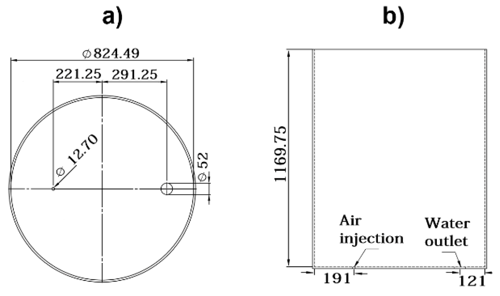
The experimental setup consisted of a 1/3 scale ladle, made of transparent plastic by a billet company located in Mexico and equipped with a bottom plug to stir steel with argon. The dimensions of the model and the positions of the plug and the slide gate are reported in Figure 1a,b. The ladle was filled with tap water through a top pipe until the operational scaled-height corresponded to the plant. The injection of argon was modeled using air supplied by an air compressor and injected through an orifice in the ladle bottom, with a pressure of 2.5 kg/cm2. The gas flow rate was measured through a mass flowmeter located between the compressor and the injection point. The lighter phase was food-oil and a layer of this material was conformed before starting the experiment to obtain the desired thickness. For visualization records of the experiments, two video cameras were placed, one on the top of the bath and another one facing the wall of a flat chamber attached outside the ladle wall filled with water to avoid optical distortions from the curvature of the vessel. The camera on the top recorded the images of the bath surface without and with an oil layer. The video recordings were decomposed into images of the eye opening with a frequency of 2 s−1. Quantitative measurements of these areas were performed, using a previously calibrated image analyzer software [28] and following a similar procedure as reported by Peranandhanthan and Mazumdar [25]. The scale down criterion to 1/3 was carried out with the equation , derived from the Froude number [29], where and are the gas flow rate in the prototype and the model, respectively, and is the scale factor.

Figure 1.
(a) Dimensions of the model (mm). (b) Position of the nozzle.
Twenty cubic centimeters of an aqueous solution of food red-colorant was employed as tracer, injected 100 mm below the bath surface near the geometric center of the ladle. A peristaltic pump was used for extracting samples from the bath, which were fed into a colorimeter cell to obtain the instantaneous concentration of the tracer. The analog signals of the colorimeter were converted into digital signals through a data acquisition card in a PC permitting real-time plotting of the tracer concentration versus time. Fluid flow turbulence was captured through a 10 million Hz ultrasonic transducer, or probe, immersed in the bath 20 mm below its surface and located in the ladle wall just opposite the wall which was nearest to the injection orifice. This probe measured the horizontal velocities in the bath at this plane, as well as all turbulent variables associated with the flow. Figure 2 shows a scheme of the experimental setup described here. The physical properties of the three phases—water, oil, and air—, as well as other details of the experimentation are shown in Table 4.

Figure 2.
Experimental set up. (a) Air compressor. (b) Water. (c) Oil layer. (d) Tracer injection. (e) Flat chamber. (f) Upper camera. (g) Ultrasonic transducer. (h) Mass flowmeter. (i) Frontal camera. (j) Colorimeter cell. (k) Air injection.
Table 4.
Experimental conditions and physical properties of the multiphase model.
3. The Multiphase Model
To simulate the interaction among the multiphase system, the VOF was applied [30]. This model uses a common pressure-velocity field by solving a single set of momentum transfer equations and uses as a phase indicator, for including the presence of interfaces, the volume fraction of a phase by the solving the corresponding advection equation. The equation of the phase indicator is,
where the unit value of αi corresponds to a cell full of fluid 1, while a zero value indicates that the cell contains no fluid 1, is the mix velocity. To avoid numerical diffusion the equation should be solved using second order explicit discretization equation in time and space, updating the indicator through the velocity field [31]. The pressure-velocity field is simulated by resolving the continuity and Navier-Stokes equations,
where the uk is the Reynolds Averaged Navier-Stokes (RANS) velocity of the turbulent flow, and and are the pressure and velocity in the direction k. The interface boundary conditions or momentum jump conditions are expressed as,
where is the total stress interfacial tensor, is the normal vector to the interfacial surface, and are the surface tension, the radius of curvature, and the normal vector to the interface which was simulated through the Continuous Surface Model of Brackbill [32]. For the present case, the physical properties of the multiphase system, (including the food-oil [33]), were calculated as,
where the sub-indexes w, o, and a hold for water, oil, and air, respectively. The k-ε model [34,35] was used to simulate the turbulence of the flow combined with Equations (2) and (3) to obtain the pressure-velocity field, which was employed to update the advection equation of the indicator. The model, which was based in the turbulent viscosity hypothesis [35], required the solution of two other equations for the turbulent kinetic energy and its dissipation rate,
Gk was the generation of kinetic energy due to the interaction between the gradients of the mean velocity and the Reynolds stresses (energy extracted from the mean flow):
And Gb is the energy generated by buoyancy forces, given by Equation (11):
The scalars k and ε are used to calculate the turbulent viscosity through Equation (12),
where Cμ = 0.09, C1ε = 1.44, C2ε = 1.92, σk = 1.0, σε = 1.3, and C3ε = 1.0.
The solution of the governing equations with the boundary conditions and all source terms were obtained through the commercial package ANSYS [36]. In all solid surfaces, a no-slip boundary condition was applied, and the wall log-law was used to link the outer grid with the computational elements in the boundary layer. In the nozzle, an entry gas-velocity boundary condition was applied and, in the top surface of the bath, a pressure one was applied. The calculation domain was divided by 2,000,000 hexahedral-100% low skewedness-structured cells, using a second order discretization scheme and a segregated-explicit coupled computing procedure. The Pressure Implicit of Splitting Operations (PISO) algorithm was employed for the pressure-velocity coupling [36]. Testing was not carried out regarding the independence of the numerical results, it was assumed that this requirement was accomplished. The calculations were conducted under transient conditions. The model was running for 300 s, ensuring a stable flow condition by reviewing the data file every 1 s. A criterion for convergence was fixed when the sum of all residuals for the dependent variables were less than 10−4 with unbalances less than 1%. It was assumed that these settings ensured independence of the numerical results from the mesh size, although analysis in this regard was not actually carried out.
4. Results and Discussion
4.1. Flow Parameters
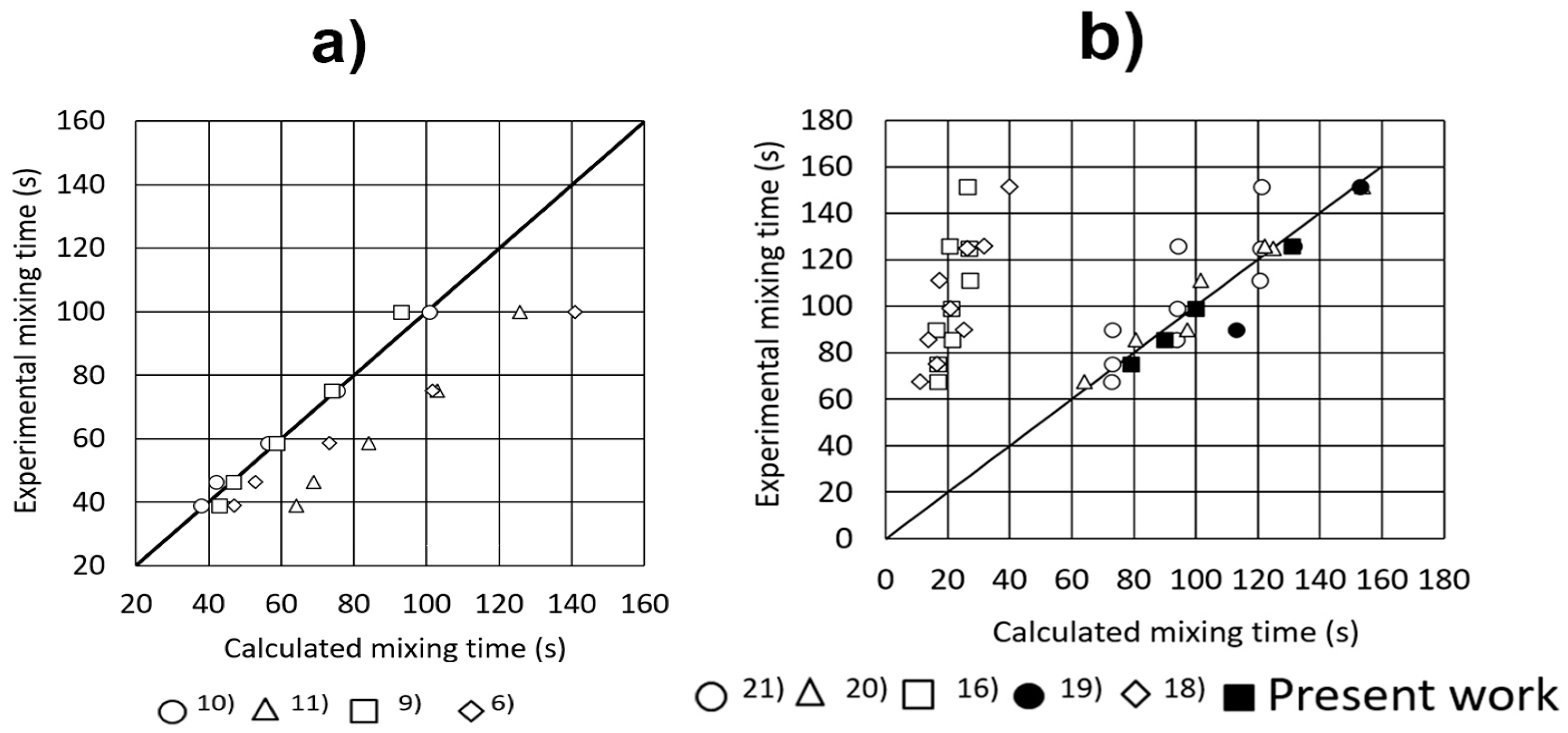
The mixing time was considered when 95% of the global tracer concentration was achieved for the two-phase flow, calculated using the experimental conditions of Table 4 and the correlations in Table 1. These calculated mixing times were compared with the corresponding experimental mixing times, and the two values plotted in Figure 3a. Here it was evident that correlations 1 and 3 in Table 1 were the most approximated to the experimental measurements. Since the presence of the upper phase affected the fluid dynamics of the lower phase, the same procedure was applied for calculating the mixing times of the three-phase system (two immiscible liquids and gas phase), using the correlations of Table 2 and comparing these values with the experimental measurements. The results are presented in Figure 3b, where, as it is evident, five predicted values are very approximated to the experimental ones. Carefully observing these two correlations for the two-phase and three-phase flows, given their highest accuracy in predicting the experimental mixing times, the following observations could be established:
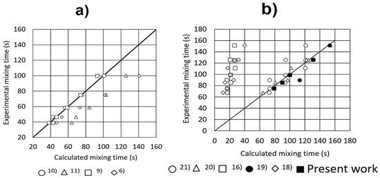
Figure 3.
Experimental versus calculated mixing times. (a) Bath without an upper layer. (b) Bath with an upper layer.
- For two-phase flows, mixing time was basically dependent on the stirring energy, the bath height, and on the geometry of the ladle.
- Tall baths favored smaller values of the mixing time.
- For three-phase flows, thicker slags increased the mixing time.
- The mixing time was basically independent from the physical properties of the upper phase, such as density and viscosity, and depends more on its thickness.
The later observation was the most oriented to discussion of what someone would intuitively think of as the physical properties of the slag or upper phase would be determinant. However, it was evident from the presented results and those of other researchers that the control of mixing was essentially the thickness due to the dissipation rate of kinetic energy when the gas–liquid plume strains the interface. That is, once the liquid, driven by the buoyancy forces imparted by the bubbles, reached the interface, the upper phase was displaced, receding toward the ladle wall and forming the spout where the bubbles burst, consuming energy in the process.
The experimental SEO areas along the experimental time are shown in Figure 4, and these areas suffered natural variations due to the turbulence of the flow but tended to reach constant values for any given operating condition.
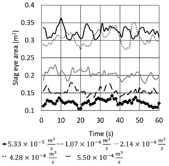
Figure 4.
Effects of gas flow rate for an upper layer thickness of 0.02 m on the variations of the eye opening area with time.
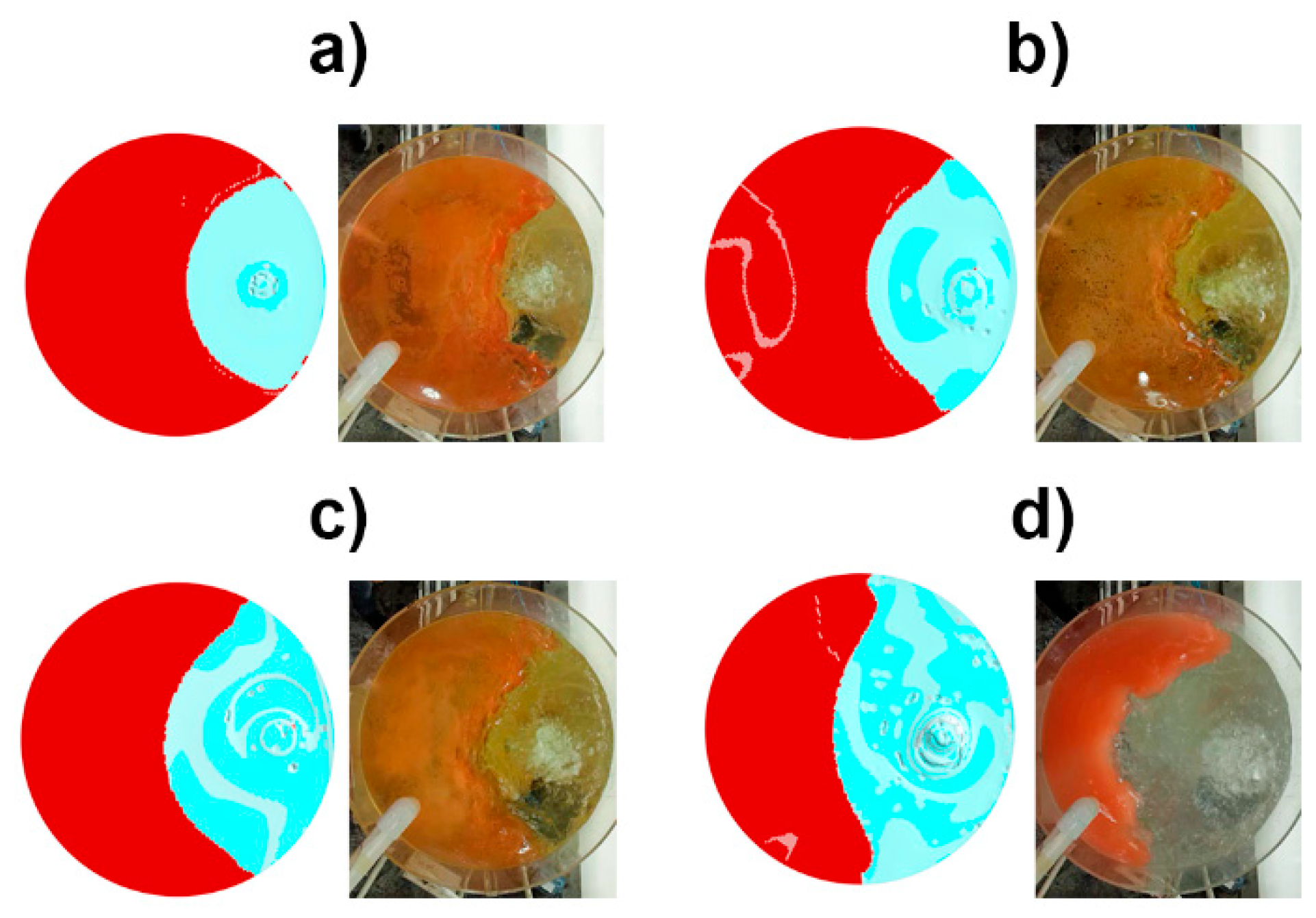
Figure 5 shows the SEO areas simulated with the mathematical model and compared with corresponding photos of the experimental SEO areas. As seen, there was a very good qualitative agreement between the mathematical simulations and the experimental SEO areas; even the shapes of the SEOs were very similar.

Figure 5.
Comparison between experimental and numerical views of the slag eye opening area for an oil thickness 0.02 m. (a) Flow 5.33 × 10⁻⁵ m3/s. (b) 1.07 × 10⁻⁴ m3/s. (c) 2.14 × 10⁻⁴ m3/s. (d) 4.28 × 10⁻⁴ m3/s.
To test the quantitative capacity of the mathematical model in predicting the experimental SEO areas, the images of the digital images and the areas of the corresponding photos in Figure 5 were measured with the image analyzer. The results of the digital or numerical SEO areas were compared with the measured SEO areas in Figure 6 and, as is seen, the agreement is excellent, granting the reliability of the mathematical model to study the dynamics of the three-phase flow system. In the same Figure, the SEO areas calculated with the correlations of Table 3, could be compared with the experimental SEOs, and it was evident that the best correlation was the number 4. Therefore, this correlation is recommended as a simple engineering tool to estimate the SEO for operating steel ladles. Accordingly, it could be said that the present mathematical model is useful in testing the reliability of engineering correlations for calculating mixing time and SEO areas.
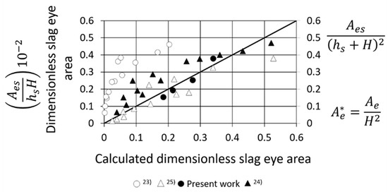
Figure 6.
Slag eye opening area.
4.2. Flow Structure
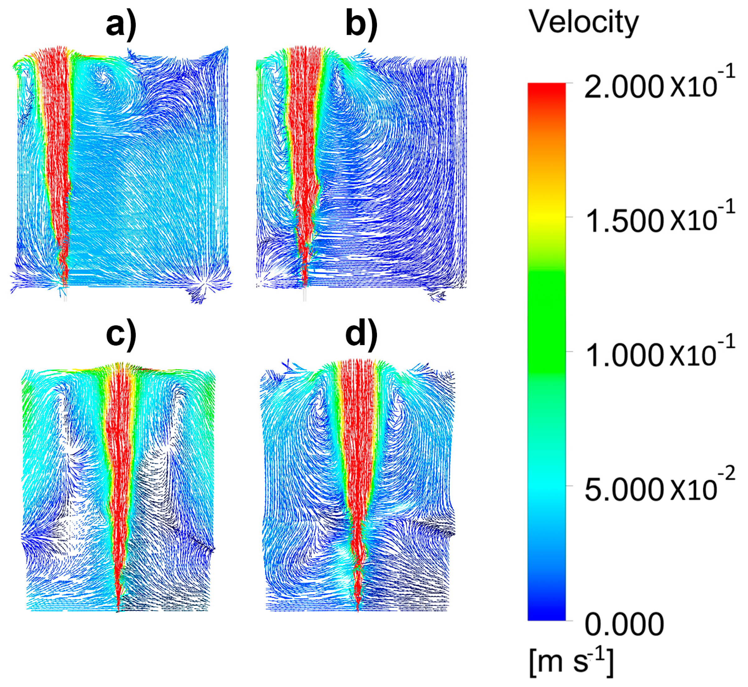
The presence of a slag or an upper layer decreased the turbulence of the denser liquid, as is seen in Figure 7a,b for the velocity field in a vertical plane passing through the axis of the injector without and with a 0.01 m thick layer, respectively. Without an upper layer, the recirculating flow was large enough to include the full plane. However, even a thin upper layer restricted the recirculating flow forming a free shear boundary layer in the upper right extreme, near the ladle wall. Figure 7c,d shows the velocity fields in perpendicular planes to those shown in Figure 7a,b.
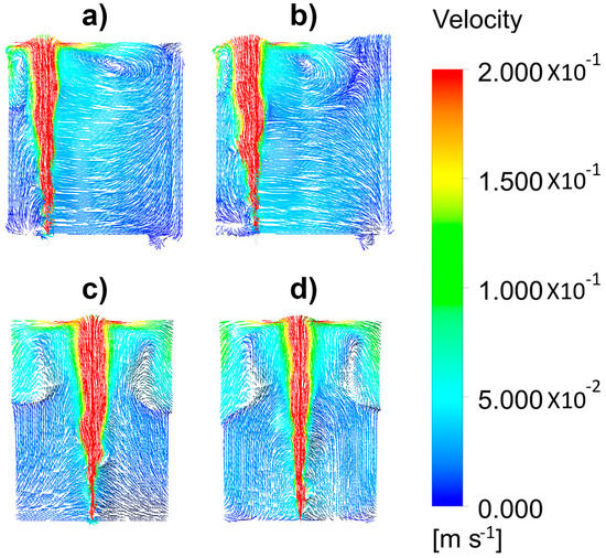
Figure 7.
Simulated velocity fields of the liquid phase for a gas flow rate of 1.07 × 10⁻⁴ m3/s and different thicknesses of the oil layer. Front view (a) 0 m and (b) 0.01 m. Side view (c) 0 m and (d) 0.01 m.
As seen, in these planes, more than half of these planes had small fluid velocities and the last third of the upper region was subjected to the effects of recirculating flows induced by the two-phase plume. Figure 8a,b correspond to Figure 7a,b with upper layer thicknesses of 0.02 and 0.04 m, respectively. The thicker upper layers constrained more the upper recirculating flow, leaving larger regions of small liquid velocities. Once the plume reached the bath surface, it encountered the upper layer, which was displaced forming the slag eye opening and the spout. Figure 8c,d show the velocity fields in planes which are perpendicular to those shown in Figure 8a,b, respectively. The regions with small velocities increased considerably; with an upper layer of 0.02 m, there was still a recirculating flow in the denser flow made contact with the upper phase. However, when the upper layer thickness was 0.04 m, the contact between the denser and upper layer was constrained to a very limited area surrounding the spout. Under these conditions the exchange between both liquid phases was very poor and, from a practical point of view, very small refining capacity was left and the capture of inclusions was limited. Since we used a 1/3 scale model, a thick 0.12 m slag would keep stagnant practically all the melt for a flow a rate of 100 l/min. An option was to increase the flow rate of argon to intensify the contact between both liquids, but thick slags were easily entrained in the melt bulk [37], increasing the presence of inclusions.
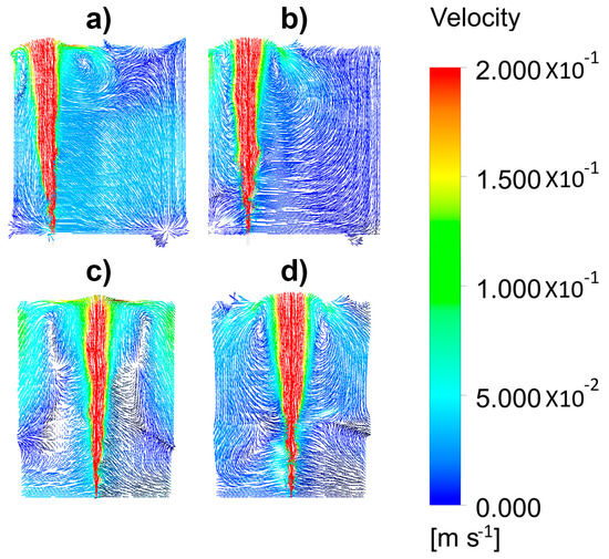
Figure 8.
Simulated velocity fields of the liquid phase for a gas flow rate of 1.07 × 10⁻⁴ m3/s and different thicknesses of the oil layer. Front view (a) 0.02 m and (b) 0.04 m. Side view (c) 0.02 m and (d) 0.04 m.
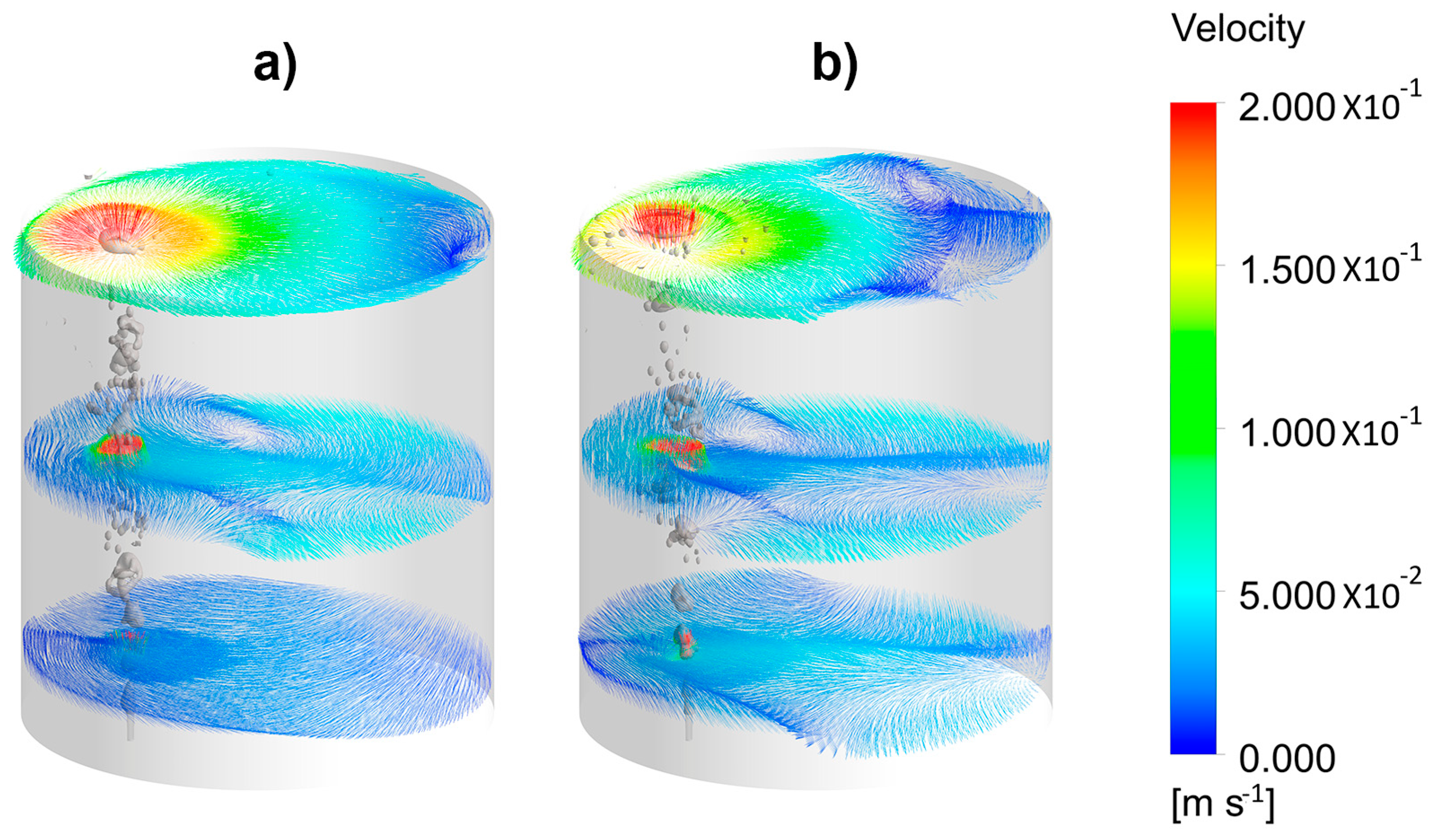
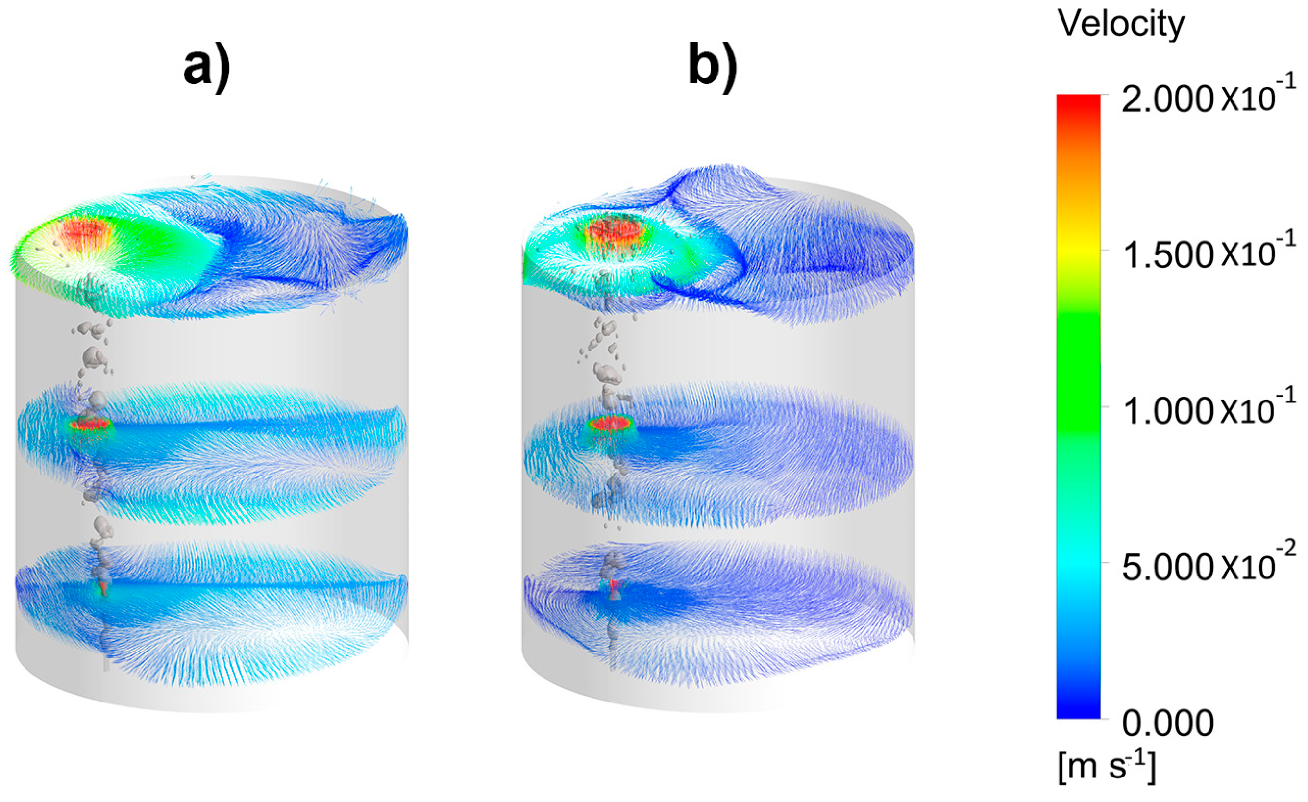
Figure 9a,b shows the velocity fields in horizontal planes at different bath heights, for a ladle without and with an upper layer 0.01 m thick. Without the upper layer, horizontal-rotating motions are observed, but even the presence of a thin upper layer changed the flow pattern to divided recirculating flows at each side of the plume. Thicker layers of 0.02 and 0.04 m in Figure 10a,b, respectively, intensified the split of the velocity fields at each side of the plume, though, with a 0.02 m thick layer, the motion in the liquid bulk was still appreciable. Hence, a layer of 0.06 m in the actual ladle was thin enough to maintain good stirring conditions and even increased the flow of rate of gas to intensify the mass transfer during the desulfurization process. This thickness represented 2.2% of the total bath height, and it would be recommendable since it kept a volume large enough to capture inclusions and to desulfurize steel. Thinner layers would not be enough to keep dissolved all the sulfur necessary for a given steel grade, and thicker slags would constrain the motion of steel, thereby decreasing its contact with the slag.

Figure 9.
Simulated velocity fields of the liquid phase in different horizontal planes, at 100 mm, 450 mm, and 880 mm, for a gas flow rate of 1.07 × 10⁻⁴ m3/s and different thicknesses of the oil layer. (a) 0 m and (b) 0.01 m.

Figure 10.
Simulated velocity fields of the liquid phase in different horizontal planes, at 100 mm, 450 mm, and 880 mm, for a gas flow rate of 1.07 × 10⁻⁴ m3/s and different thicknesses of the oil layer. (a) 0.02 m and (b) 0.04 m.
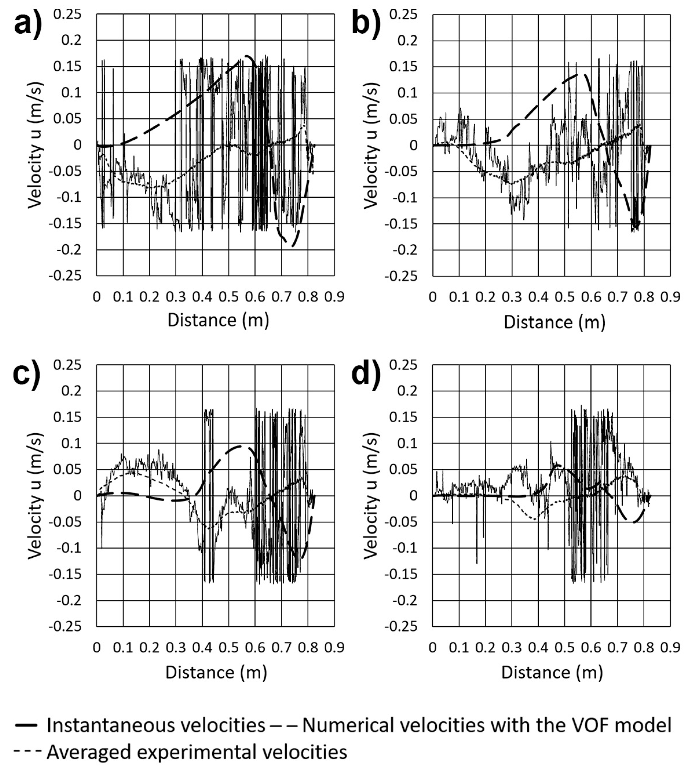
The proximities of the metal-slag interface are the most important to capture inclusions by the slag phase. Therefore, it is important to understand the turbulence conditions in this region. Figure 11a–d show the measured horizontal-velocities with the ultrasound probe along the distance from the opposite wall of the plume to the wall behind the plume. The dotted line corresponds to the average velocities of the experimental measurements, and the interrupted lines correspond to the predictions of the mathematical model. When there was not an upper layer, as in Figure 11a, the velocity fluctuations near the wall were large and their amplitudes grew at a maximum at the location of the plume, due to the bursting effect of the bubbles. Even under the presence of a thin layer, as in Figure 11b, the velocity fluctuations were considerably damped and remained large in the region of the plume for the reason adduced above. As the layer got thicker, as in Figure 11c,d, the velocity fluctuations suffered further dampening to the point where there were practically no more, and leaving only those velocity spikes corresponding to the plume. Regarding the mathematical model, although its predictions do not match as well the averaged experimental velocities, they lay inside the magnitudes of the fluctuating velocities. The reasons of this mismatch are basically three, the first is that the VOF model solves only one set of equations for all three phases, and the second is that this model predicts averaged velocities of turbulent flows. The third reason is the impossibility to match the computing time with the experimental ones. All these factors impede a good matching between simulations and measurements. However, given these upheavals the mathematical model makes predictions of the trends of the velocity fields. Another possible source of error could be the nit independence of the numerical results from mesh size.

Figure 11.
Measured versus simulated velocities 20 mm below the metal-slag interface for different thicknesses of the upper phase layer at a fixed gas flow rate of 1.07 × 10⁻⁴ m3/s. (a) 0 m, (b) 0.01 m, (c) 0.02 m, and (d) 0.04 m.
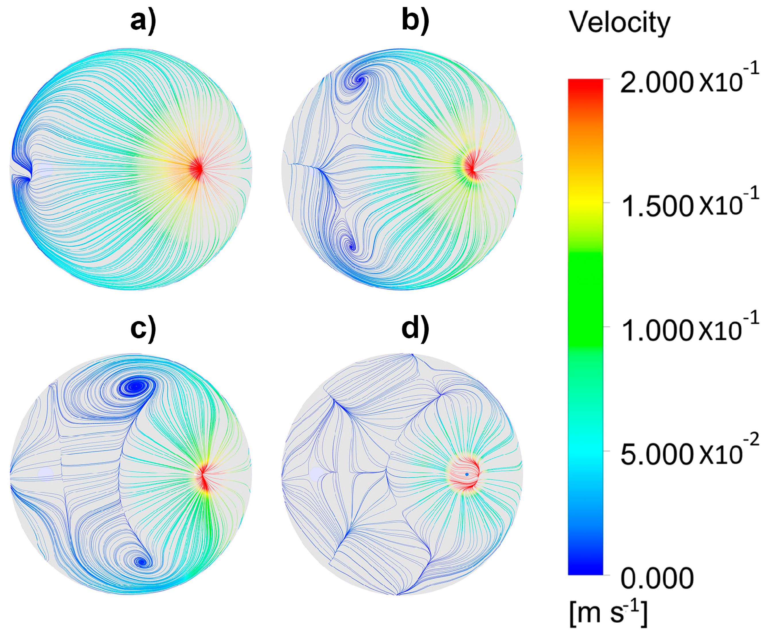
Further information about the flow structure in proximities of the metal-slag interface c be seen through the fields of streamlines shown in Figure 12a–d corresponding to Figure 11a–d, respectively. With no upper layer, the stream lines initiating from the spout followed a regular irradiating pattern. With a thin layer, this pattern was slightly disrupted, and two regular vortexes were formed symmetrically and close to the opposite ladle wall. Thicker layers subdivided the flow in many local vortexes with different orientations, making the flow practically stagnant.
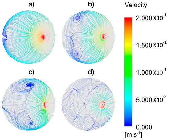
Figure 12.
Streamlines of the flow for different thicknesses of the upper layer for a gas flow rate of 1.07 × 10⁻⁴ m3/s. (a) 0 m, (b) 0.01 m, (c) 0.02 m, and (d) 0.04 m.
4.3. Closure
Despite the limitations of the model, made explicit before, it was evident that mixing times are dependent on stirring energy and bath geometry in two-phase flows. In three phase flows, mixing time depends on these factors and on the thickness of the slag phase, the physical properties of the upper layer play a secondary role. The SEO area in three-phase flows depends on the flow rate of the stirring gas, the physical properties of the upper layer and on the bath height. As the thickness of the upper layer increases, the mixing time increases and the bath approaches near-stagnant condition. The SEO area increases with the flow rate of gas and decreases with the slag thickness. Denser upper layers favor larger SEO areas and high viscosity layers decrease it.
There has been research claiming that bubbles play an important role to float out inclusions through mechanism of their adherence on their surfaces [38] and carrying them to the bath surface. Rather, it is the motion of steel, originated by the energy provided by the buoyant bubbles, that carries the inclusions in contact with the slag which, eventually, absorbs them. Hence, it was difficult to agree with this view, as their area volume ratio is very small, as can be seen in Figure 9 and Figure 10. It could be criticized that these simulations do not reflect actual sizes in liquid steel. However, water models always report big bubbles sizes, that may or may not be disintegrated, and given the surface tension of liquid steel, argon bubbles in steel should be twice as large as those observed in the models. Instead, it is the flow near the proximities of the metal–slag-interface which control the floatation of inclusions. When this region is disrupted by strong forced convection flows, the efficiency of floatation decreases. It is only when this region comes to some velocity fields of small magnitude that the efficiency to float inclusions gets high. This explains the need of having what it is called “rinsing time”, which refers to the last period after refining, when the stirring energy is decreased to allow floatation of inclusions in the Stokes regime. This operation is well-known by all steelmakers, and it is certainly a very necessary one to attain the best of steel cleanliness.
Author Contributions
Investigation, F.A.C.-H. and S.G.-H.; Methodology, R.M.D.; Supervision, K.C.
Funding
This research was funded by Consejo Nacional de Ciencia y Tecnología (CoNaCyT).
Acknowledgments
We give the thanks to IPN and (CoNaCyT) for the support of this work. One of us (R.M.) gives the thanks to University of Toronto for making his stay in Toronto possible.
Conflicts of Interest
The authors declare no conflict of interest.
Abbreviations
List of Symbols
| , —Slag eye opening area |
| —Area of the plume |
| —Velocity in direction “” |
| and —Gas flow rate |
| —Ladle height |
| —Ladle radius |
| —Plume velocity |
| —Ladle diameter |
| —Thickness of the oil or slag layer |
| —Effective bath height |
| —Number of plugs or orifices in the ladle bottom |
| —Radial position |
| —Interfacial stress tensor |
| —Normal vector to the interfacial surface |
| , —Bath height |
| —Turbulent kinetic energy |
| and —the generation terms of kinetic energy by the mean flow and by the buoyancy, respectively. |
| —Gravity constant |
| Pr—Prandtl number |
Greek Letters
| Volume fraction of phase “i” |
| Mixing time |
| —Specific potential energy input |
| Density of phase “i” |
| ε—Dissipation rate of turbulent kinetic energy |
| Kinematic viscosity of phase “i” |
| Surface tension |
| —Dynamic viscosity of the slag |
Sub-Indexes
| m.—mixture |
| s.—slag |
| o.—oil |
| w.—water |
References
- Krishnapisharody, K.; Irons, G.A. A Model for Slag Eyes in Steel Refining Ladles Covered with Thick Slag. Metall. Mater. Trans. B 2015, 46, 191–198. [Google Scholar] [CrossRef]
- Krishnapisharody, K.; Irons, G.A. Modeling of Slag Eye Formation over a Metal Bath Due to Gas Bubbling. Metall. Mater. Trans. B 2006, 37, 763–772. [Google Scholar] [CrossRef]
- Krishnapisharody, K.; Irons, G.A. A Study of Spouts on Bath Surfaces from Gas Bubbling: Part II. Elucidation of Plume Dynamics. Metall. Mater. Trans. B 2007, 38, 377–388. [Google Scholar] [CrossRef]
- Krishnapisharody, K.; Irons, G.A. A Study of Spouts on Bath Surfaces from Gas Bubbling: Part I. Experimental Investigation. Metall. Mater. Trans. B 2007, 38, 367–375. [Google Scholar] [CrossRef]
- Krishnapisharody, K.; Irons, G.A. A Unified Approach to the Fluid Dynamics of Gas–Liquid Plumes in Ladle Metallurgy. ISIJ Int. 2010, 50, 1413–1421. [Google Scholar] [CrossRef]
- Iguchi, M.; Nakamura, K.; Tsujino, R. Mixing Time and Fluid Flow Phenomena in Liquids of Varying Kinematic Viscosities Agitated by Bottom Gas Injection. Metall. Mater. Trans. B 1998, 29, 569. [Google Scholar] [CrossRef]
- Mazumdar, D.; Guthrie, R.I.L. Discussion of “mixing time and fluid flow phenomena in liquids of varying kinematic viscosities agitated by bottom gas injection”. Metall. Mater. Trans. B 1999, 30, 349–351. [Google Scholar] [CrossRef]
- Mazumdar, D.; Guthrie, R.I.L. Hydrodynamic modeling of some gas injection procedures in ladle metallurgy operations. Metall. Mater. Trans. B 1985, 16, 83–90. [Google Scholar] [CrossRef]
- Mazumdar, D.; Guthrie, R.I.L. Mixing models for gas stirred metallurgical reactors. Metall. Mater. Trans. B 1986, 17, 725–733. [Google Scholar] [CrossRef]
- Haida, O.; Emi, T.; Yamada, S.; Sudo, F. Scaninjet II, Part I. In Proceedings of the 2nd International Conference on Injection Metallurgy, MEFOS-Jerkentoret, Lulea, Sweden, 12–13 June 1980. [Google Scholar]
- Ying, Q.; Yun, L.; Liu, L. Scaninjet III, Part I. In Proceedings of the 2nd International Conference on Injection Metallurgy, MEFOS-Jernkontoret, Lulea, Sweden, 15–17 June 1983. [Google Scholar]
- Li, B.; Yin, H.; Zhou, C.Q.; Tsukihashi, F. Modeling of Three-phase Flows and Behavior of Slag/Steel Interface in an Argon Gas Stirred Ladle. ISIJ Int. 2008, 48, 1704–1711. [Google Scholar] [CrossRef]
- Liu, Z.; Li, L.; Li, B. ISIJ International, Modeling of Gas-Steel-Slag Three-Phase Flow in Ladle Metallurgy: Part I. Phys. Model. 2017, 57, 1971. [Google Scholar]
- Singh, U.; Anapagaddi, R.; Mangal, S.; Padmanabhan, K.A.; Singh, A.K. Multiphase Modeling of Bottom-Stirred Ladle for Prediction of Slag–Steel Interface and Estimation of Desulfurization Behavior. Metall. Mater. Trans. B 2016, 47, 1804–1816. [Google Scholar] [CrossRef]
- Mazumdar, D.; Guthrie, R.I.L. Modeling Energy Dissipation in Slag-Covered Steel Baths in Steelmaking Ladles. Metall. Mater. Trans. B 2010, 41, 976–989. [Google Scholar] [CrossRef]
- Khajavi, L.T.; Barati, M. Liquid Mixing in Thick-Slag-Covered Metallurgical Baths—Blending of Bath. Metall. Mater. Trans. B 2010, 41, 86–93. [Google Scholar] [CrossRef]
- Jonsson, P.G.; Sichen, D. Viscosities of LF Slags and Their Impact on Ladle Refining. ISIJ Int. 1997, 37, 484–491. [Google Scholar] [CrossRef]
- Yamashita, S.; Miyamoto, K.; Iguchi, M.; Zeze, M. Model Experiments on the Mixing Time in a Bottom Blown Bath Covered with Top Slag. ISIJ Int. 2003, 43, 1858–1860. [Google Scholar] [CrossRef]
- Mazumdar, D.; Kumar, D.S. In Proceedings: Oxygen in Steelmaking; Irons, G., Sun, S., Eds.; MetSoc of CIM: Westmount, QC, Canada, 2004; pp. 311–323. [Google Scholar]
- Patil, S.P.; Satish, D.; Peranandhanthan, M.; Mazumdar, D. Mixing Models for Slag Covered, Argon Stirred Ladles. ISIJ Int. 2010, 50, 1117–1124. [Google Scholar] [CrossRef]
- Amaro-Villeda, A.M.; Ramirez-Argaez, M.A.; Conejo, A.N. Effect of Slag Properties on Mixing Phenomena in Gas-stirred Ladles by Physical Modeling. ISIJ Int. 2014, 54, 1–8. [Google Scholar] [CrossRef]
- Yonezawa, K.; Schwerdtfeger, K. Spout eyes formed by an emerging gas plume at the surface of a slag-covered metal melt. Metall. Trans. 1999, 30, 411–418. [Google Scholar] [CrossRef]
- Subagyo, G.A.; Brooks, G.A. Irons. Spout Eyes Area Correlation in Ladle Metallurgy. ISIJ Int. 2003, 43, 262–263. [Google Scholar] [CrossRef]
- Krishnapisharody, K.; Irons, G.A. An Extended Model for Slag Eye Size in Ladle Metallurgy. ISIJ Int. 2008, 48, 1807–1809. [Google Scholar] [CrossRef]
- Peranandhanthan, M.; Mazumdar, D. Modeling of Slag Eye Area in Argon Stirred Ladles. ISIJ Int. 2010, 50, 1622–1631. [Google Scholar] [CrossRef]
- Liu, W.; Tang, H.; Yang, S.; Wang, M.; Li, J.; Li, Q.; Liu, J. Numerical Simulation of Slag Eye Formation and Slag Entrapment in a Bottom-Blown Argon-Stirred Ladle. Metall. Trans. B 2018, 49, 2681–2691. [Google Scholar] [CrossRef]
- Ramasetti, E.; Visuri, V.-V.; Sulasalmi, P.; Mattila, R.; Fabritius, T. Modeling of the Effect of the Gas Flow Rate on the Fluid Flow and Open-Eye Formation in a Water Model of a Steelmaking Ladle. Steel Res. Int. 2018, 90. [Google Scholar] [CrossRef]
- Image Processing and Analysis in Java. Consulted in October 2018. Available online: http://imagej.nih.gov/ij/index.html. ImageJ-1.49 (accessed on 5 October 2018 ).
- Frank, M. White, Fluid Mechanics, 4th ed.; McGraw-Hill: New York, NY, USA, 1999; p. 294. [Google Scholar]
- Hirt, C.W.; Nichols, B.D. Volume of fluid (VOF) method for the dynamics of free boundaries. J. Comput. Phys. 1981, 39, 201–225. [Google Scholar] [CrossRef]
- Ferziger, J.H.; Peric, M. Computational Methods for Fluid Dynamics; Springer: Berlin, Germany; New York, NY, USA, 2002; pp. 72–75. [Google Scholar]
- Brackbill, J.U.; Kothe, D.B.; Zemach, C. A continuum method for modeling surface tension. J. Comput. Phys. 1992, 100, 335–354. [Google Scholar] [CrossRef]
- Sahasrabudhe, S.N.; Rodriguez-Martinez, V.; O’Meara, M.; Frakas, B.E. Density, viscosity, and surface tension of five vegetable oils at elevated temperatures: Measurement and modeling. Int. J. Food Prop. 2017, 20, S1965–S1981. [Google Scholar] [CrossRef]
- Pope, S.B. Turbulent Flows; Cambridge Press: New York, NY, USA; Cambridge, UK; London, UK, 2000; pp. 387–457. [Google Scholar]
- Wilcox, D.C. Turbulence Modeling for CFD; D.C.W. Industries Inc: La Cañada, CA, USA, 2000; pp. 103–218. [Google Scholar]
- ANSYS-FLUENT. Available online: www. ansys.com/Products/Fluids/ANSYS-Fluent (accessed on 3 May 2018).
- Han, Z.; Holappa, L. Mechanisms of Iron Entrainment into Slag due to Rising Gas Bubbles. ISIJ Int. 2003, 43, 292–297. [Google Scholar] [CrossRef]
- Soder, M.; Jonsson, P.; Jonsson, L. Inclusion Growth and Removal in Gas-Stirred Ladles. Steel Res. Int. 2004, 75, 128–138. [Google Scholar] [CrossRef]


© 2019 by the authors. Licensee MDPI, Basel, Switzerland. This article is an open access article distributed under the terms and conditions of the Creative Commons Attribution (CC BY) license (http://creativecommons.org/licenses/by/4.0/).