Abstract
For the flexible multi-point stretch-bending forming process, which involves complex forming procedures, finite element (FE) modeling can significantly reduce trial-and-error costs and provide a convenient means for determining process parameters in actual production. During the creation of FE models, simplifying the material model is crucial: insufficient simplification greatly increases computation time, while excessive simplification reduces model accuracy. This study establishes user material subroutines in the FE simulation software Abaqus to introduce anisotropic yield models, specifically Hill’s 48 and Yld2004-18p models. Multi-point stretch-bending experiments were repeated and compared with simulations using the traditional isotropic Von Mises yield model to analyze the impact of isotropic simplification on the accuracy of forming results. The applicability of isotropic simplification under different degrees of deformation is investigated, and the fundamental causes of errors are analyzed. Ultimately, the error response of the material simplified model is obtained. This provides an error reduction scheme for subsequent research using the isotropic simplified model.
1. Introduction
Metal profiles are widely used in industries such as automotive, aerospace, and rail transportation manufacturing. The plastic forming process involves applying external forces to metal profile blanks to achieve the desired shapes. Among these, the stretch-bending forming process is widely used for bending workpieces due to its superior dimensional accuracy [1]. However, traditional profile stretch-bending processes require expensive dies to obtain the desired shapes. And any adjustments to process parameters necessitate the manufacture of new dies, significantly increasing production costs [2]. Furthermore, with the growing demand for products, profiles with three-dimensional bending deformations are also in greater demand. To address these issues, Liang et al. [3] proposed the Flexible Stretch-Bending Forming process with Roller Dies (FSBRD), which is based on flexible multi-point forming technology [4,5]. This process discretizes the overall die, enabling rapid reconstruction and adjustment of the formed shape. As a result, the blank can achieve ideal bending deformation with high efficiency, flexible operation, and a short development cycle. Additionally, using roller-type dies instead of the traditional flat die in the flexible multi-point bending process results in better forming outcomes.
Simulation analysis plays a crucial role in the development of forming processes, as it can visualize otherwise invisible phenomena and predict process outcomes. It is one of the main components of the digital design and manufacturing of industrial products [6]. Wang et al. [7] developed a simulation model for wrinkles-free forming of metal sheets using a low-melting-point alloy medium via FE software Abaqus. They investigated the effects of process parameters, forming temperature, and medium rheological behavior on the forming results. Marko et al. [8] proposed a new constitutive model to simulate the deformation process in the study of sheet metal bending springback. This model takes into account anisotropy, strain path-dependent stiffness degradation and damage evolution during plastic deformation. The simulation results obtained are in good agreement with the experimental results. Liu et al. [9] proposed a multiple-tool modeling method to reduce the FE simulation computation time for incremental sheet forming processes. In this method, the computational efficiency can be increased by artificially adding more forming tools in the FE model in a way that shortens individual forming toolpaths. This is achieved by multiple pairs of tools moving simultaneously according to predefined split toolpath segments. Compared to traditional FE models, this method reduced CPU time by up to 90% while still maintaining good geometric accuracy.
When constructing FE models, differences in material constitutive properties have a significant impact on the process and results of the analysis [10,11]. Using more accurate material constitutive properties can better replicate the forming process, yielding simulation results that closely match experimental outcomes. However, this often leads to more computational steps and longer processing times. Simplifying material properties within certain limits can yield faster simulation results but may cause discrepancies with experimental results [12]. Therefore, seeking a computational model that balances speed with accuracy, within an acceptable error range, can improve both the quality of the results and work efficiency. Chen et al. [13] investigated the influence of the strain hardening exponent on sidewall curling and angle variation in U-shaped grooves by studying a U-tube forming model based on the finite element method. N’Jock et al. [14] proposed a fully coupled damage model that takes anisotropy into account for predicting the springback of advanced high-strength steels. Ma et al. [15] accurately predicted the springback in the aluminum bending tube process by modifying the plastic constitutive equation for hot forming, thereby improving product precision. Liao et al. [16] analyzed the isotropic and kinematic hardening of materials, incorporating the Von Mises, Hill’s 48, and Yld2000-2d plastic yield criteria, to experimentally and numerically study the springback and torsion deformation of asymmetric AA6060-T4 aluminum tubes during rotary tensile bending. Rasoul et al. [17] additionally introduced the Yld2004-18p plastic yield criterion to study the single-point incremental forming process. Rong et al. [18] conducted simulations of hot cup drawing of AA7075 alloy at different temperatures, and it was found that the spatial fluctuation of the earing profiles can be precisely predicted by implementing the Yld2004-18p function in drawing simulations.
This study aims to investigate the FSBRD process by comparing the forming result errors caused by the Von Mises, Hill’s 48, and Yld2004-18p yield criteria to verify the suitability of the isotropic simplification in flexible bending forming processes. Material parameters are obtained through experiments and imported into the FE analysis software Abaqus 2017. Different yield models are introduced for comparative analysis using the user-defined material subroutines (Umat/Vumat). The results are then validated through practical experiments. The applicability of isotropic simplification under different degrees of deformation is investigated, and the fundamental causes of errors are analyzed. Ultimately, the error response of the material simplified model is obtained. This provides an error reduction scheme for subsequent research using the isotropic simplified model.
2. Establishment of the FE Model
2.1. FSBRD Equipment and Basic FE Model
The FSBRD equipment, by discretizing the overall die and using roller-type dies, can effectively enhance the equipment’s rapid shape adjustment capabilities while minimizing local defects caused by the discretization of the contact area. In this study, to investigate the differences caused by various material models, it is necessary to conduct experiments on deformation processes with multiple different process parameters. Therefore, this equipment is well-suited for achieving the objective. To establish the FE model, this study incorporates the equipment into the Abaqus FE analysis software and builds the model for analysis, as shown in Figure 1 below.
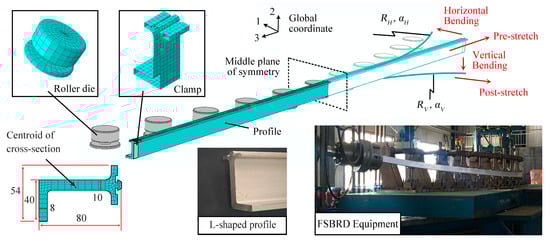
Figure 1.
FSBRD equipment and FE model.
As shown in the figure, the simulation analysis is conducted for the bending process of an aluminum alloy extruded profile with an L-shaped cross-section (where small fillets are ignored). During the bending process, the profile is clamped and undergoes deformation under applied forces, typically involving three steps: pre-stretching, bending forming, and post-stretching. Due to its unique 3D forming capability, the FSBRD equipment divides the bending forming process into two separate bending steps: horizontal bending and vertical bending. These correspond to the process where the profile approaches the dies in the horizontal direction and the profile bends along the vertical direction with the dies. In the FSBRD process, arbitrary 3D bending deformations can be achieved by adjusting the unit cells. To simplify the problem, only arc-shaped bending is considered, with horizontal and vertical bending radii and angles defined as αH, RH and αV, RV, respectively.
During the establishment of the simulation analysis model, given the complexity and the significant extent of deformation, the Abaqus/Explicit module is chosen for simulating the deformation process. The deformation results are then imported into the Abaqus/Standard implicit analysis module to release all loads and apply fixed constraints to the central symmetry plane for analyzing the springback results. In the explicit analysis, a friction factor of 0.15 and a mass scaling factor of 300 are used to simulate the deformation process [3].
2.2. Material Model
The selection of an appropriate material model is a crucial foundation for simulating the plastic forming process. This study focuses on the room-temperature bending process of aluminum alloy profiles, and therefore, an elastic-plastic model is used to describe the material’s deformation behavior. For purely elastic deformation, Hooke’s Law is applied. Once the material enters the plastic stage, the Swift hardening equation is used to describe the true stress–true strain relationship. Hence, the uniaxial elastic-plastic constitutive model, which relates stress σ to strain ε, is given by:
where E is the Young’s modulus, K0 is the strength coefficient, n0 is the strain hardening exponent, ε0 is the hardening equation coefficient, and εe represents the elastic limit strain. When the material reaches the elastic strain limit, plastic yielding occurs, and the corresponding yield stress is denoted as σy. Different plastic yield models will affect the judgment of the yield surface and the subsequent plastic flow in various ways. The Von Mises yield model is a commonly used yield criterion, and its stress tensor expression is as follows:
Here, σi represents the normal stress, and σij represents the shear stress (where i, j = x, y, z, and the same applies below). When the equivalent stress is less than the yield stress σy, elastic deformation occurs; otherwise, plastic deformation takes place. The Von Mises yield model is often used to describe isotropic yielding materials. However, to describe the yielding process of anisotropic materials, Hill’s 48 yield model is widely applied. The Hill’s 48 yield function is expressed as follows:
Here, the six anisotropic parameters F, G, H, L, M and N can be computed using the anisotropy coefficients Rθ, where θ represents the angle between the reference direction and the specific direction under consideration. When the parameters F, G and H are set to 0.5 and L, M and N are set to 1.5, the Hill’s 48 yield model reduces to the isotropic Von Mises yield model.
Barlat et al. [19] proposed the Yld2004-18p yield model to describe the yielding behavior of metals under three-dimensional stress states. The model is expressed as follows:
Here, for BCC and FCC structured materials, the parameter a is taken as 6 and 8, respectively. In the formula, and are the principal values of the stress after two linear transformations, denoted as and :
In the equation, σ represents the stress tensor σij, the matrices C′ and C″ represent the anisotropic coefficient matrices, and T is the transformation matrix [19]. After performing the mathematical operations on the above expression, the parameter matrices L′ and L″ are obtained as follows:
Here, the 18 parameters in the parameter matrix characterize the material’s anisotropy. In this study, seven different uniaxial tensile data from various sampling directions are used, including the normalized stress σθ/σ0 in each direction and the plastic anisotropy coefficient Rθ, to solve for the above parameters.
2.3. Implementation of User-Defined Material Subroutine
In the Abaqus FE analysis module, to introduce a more complex material model, it is often necessary to establish a user-defined material subroutine, specifically the UMAT/VUMAT module. Since the FSBRD forming process is a dynamic problem, this paper chooses the VUMAT module for solving and establishes a complete elastoplastic material model to implement the simulation process. The springback analysis process is solved implicitly, so the corresponding UMAT subroutine is established for this solution. In the explicit analysis process, the FE software computes the stress–strain state at time t (σt, εt) and the strain increment (Δεt), so the analysis process is equivalent to solving the stress state (σt+Δt) after an arbitrary time increment (Δt). This paper uses the trial stress method for solving, and the plastic flow process is solved using the stress update algorithm based on plastic incremental theory proposed by Abedrabbo et al. [20].
For the deformation process at any time t, it is assumed that pure elastic deformation has occurred. According to the generalized Hooke’s law, the trial stress σtrt+Δt satisfies the following:
where C represents the elastic stiffness matrix, which is calculated based on the material’s Young’s modulus E and Poisson’s ratio μ. The operator ‘:’ represents the double dot product. The trial stress σtrt+Δt, obtained from the calculation, is substituted into the yield criterion Equations (2) to (4) and compared with the yield stress to determine whether the material has entered the yielding state at that time. The yield stress at the current time is calculated by substituting the equivalent strain into Equation (1). Thus, the criterion for determining whether the material has yielded is as follows:
When the above equation is less than zero, it indicates that the material element is still in an elastic state at this time, so the trial stress σtrt+Δt is the desired stress σt+Δt at the current time, and the solution process ends. When the above equation is greater than or equal to zero, it indicates that plastic yielding has occurred, and the plastic multiplier must be iteratively solved to determine the material’s flow behavior after yielding. The equation is given as follows:
where i represents the iteration count, and represents the equivalent plastic strain. By substituting this into the plastic flow rule, the following stress–strain update is obtained:
The equivalent stress after iteration and the yield stress are substituted into the previous criterion, Equation (8). When the value becomes smaller than a number approaching zero (in this study, 1 × 10⁻⁷), the iterative solution is considered complete. At this point, and are the stress tensor and equivalent plastic strain at this time step. For the Yld2004-18p model, it is difficult to directly solve , so the decomposition process proposed by Barlat et al. [19] is adopted as follows:
The above process is programmed to be carried out, and the process is shown in Figure 2 below:
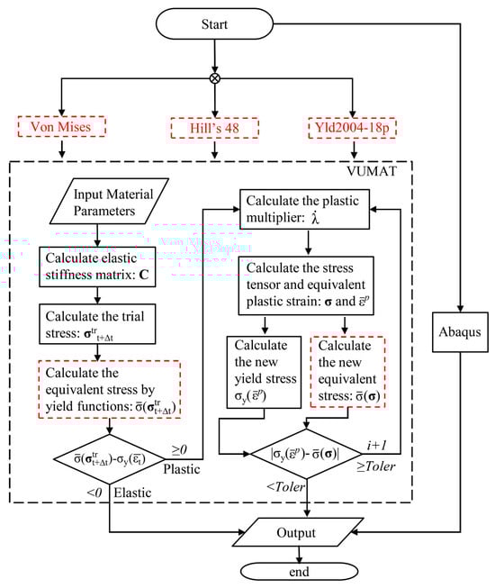
Figure 2.
Flowchart of user-defined material subroutine.
2.4. Determination of Material Parameters and Program Realization
This study uses Al6005A-T6 aluminum alloy profiles with an L-shaped cross-section for experimentation to obtain the relevant parameters necessary for constructing yield models. Different anisotropic yield models require corresponding anisotropic parameters, including normalized yield stress σθ/σ0 and plastic anisotropy values Rθ for different stretching directions. Since the selected L-shaped section profile is extruded, there are significant material property differences between the Extrusion Direction (ED) and other directions, while the material properties within the section are nearly uniform. For the profile with a large flat plate, tensile test specimens were made at angles from 0° to 90° relative to the ED, with intervals of 15°, as shown in Figure 3. In these tests, the initial yield stress in the ED was σ0 = 272 MPa. The corresponding normalized yield stress parameters in different directions are shown in Table 1. Additionally, tensile tests were performed on specimens in various directions to measure the strain ratios of width and thickness after deformation, which were used to calculate the plastic anisotropy Rθ values.
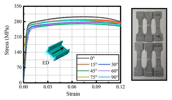
Figure 3.
True stress–true strain curves of uniaxial tension in different directions.

Table 1.
Experimental tensile test data.
The parameters of the Hill’s 48 yield model are determined using the following method:
And in the Yld2004-18p yield model, the parameters c′ij and c″ij are obtained through an error function as follows:
In the equation, the superscript pr represents the corresponding predicted values, exp represents the corresponding experimental values, and w represents the corresponding weights. In the calculations in this study, the weights for flow stress and the anisotropy coefficient R are taken as 1 and 0.1, respectively. To solve for the theoretically predicted values of yield stress and the anisotropy coefficient R for different directions, the stress variation equation σθ and the anisotropy coefficient Rθ under uniaxial tensile conditions for any direction θ are introduced:
In this study, based on the significant differences between the ED of the extruded profile and other directions, the Transverse Direction and Normal Direction are assumed to be approximately equal. Therefore, it is assumed that the two parameters L and M in Hill’s 48 yield model, which consider the out-of-plane stress conditions, are the same as in the isotropic case and are taken as 1.5. Additionally, in the Yld2004-18p yield model, the parameters are set as c′44 = c′55 = c′66 and c″44 = c″55 = c″66. Furthermore, since aluminum alloy is chosen as the material, the parameter a is taken as 8. The corresponding anisotropic parameters are then calculated and are presented in Table 2.
Table 2.
Coefficients of the yield functions Hill’s 48 and Yld2004-18p.
By substituting the obtained anisotropic model into Equation (13), the normalized yield stress and anisotropy coefficient for any direction can be calculated. The resulting curves are shown in Figure 4. From the figure, it can be observed that the sampling test results in different directions show that the selected L-profile has a certain anisotropy in the plastic stage. The Hill’s 48 yield model can characterize this anisotropy to some extent, but with a relatively large error. In contrast, the Yld2004-18p model provides a more accurate representation of the material’s anisotropy.
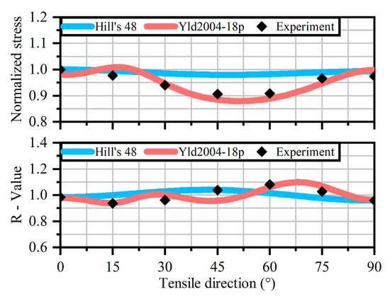
Figure 4.
Normalized stress and anisotropy coefficients under Hill’s 48 and Yld2004-18p yield models at different stretching angles, along with the experimental data.
In this paper, the above process is programmed and implemented using Fortran as shown in Figure 5. In the figure, ‘a*b’ represents a multiplied by b, and ‘a**b’ represents a to the power of b.
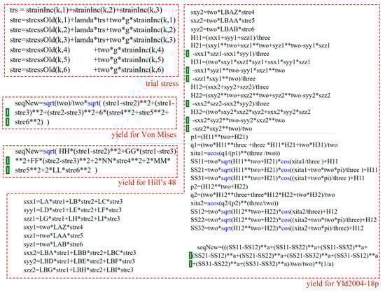
Figure 5.
Code of trial stress and different yield models.
3. Results and Discussion
3.1. Results of FE Model
Based on the FE model established earlier, simulations were first conducted using the built-in Von Mises yield model in the software. Figure 6 shows the deformation results at different analysis steps for a 30° horizontal bend and a 15° vertical bend, with both pre-stretching and post-stretching strain rates set at 1%. As observed in the figure, after the bending process, the stress distribution in the blank becomes highly uneven, with significant local stress concentration near the roller contact area. Comparing Figure 6c,d, the maximum equivalent stress increases from 3.10 × 10² MPa to 3.22 × 10² MPa, yet the overall internal stress distribution becomes more uniform, with no obvious stress concentration. This indicates that the introduction of post-stretching can effectively improve the uniformity of the stress distribution within the blank without significantly increasing the maximum stress.
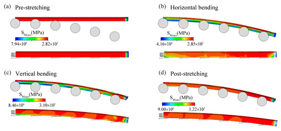
Figure 6.
Deformation of different steps for horizontal bending at 30° and vertical bending at 15°. (a) Pre-stretching step; (b) Horizontal bending step; (c) Vertical bending step; (d) Post-stretching step.
Based on the analysis of the bending forming model under the aforementioned process parameters, this study further conducts FE analysis using Hill’s 48 and Yld2004-18p yield models and compares them with the Von Mises isotropic yield model. The plane near the clamps is selected as the reference plane, and the stress–strain behavior at the center of the cross-section is compared. The results are shown in Figure 7. The horizontal axis of the curve represents the analysis step time, with analysis steps 1 to 4 corresponding to the pre-stretching, horizontal bending, vertical bending, and post-stretching stages, respectively. By observing the equivalent stress curves, it can be seen that in the first half of analysis step 1, the equivalent stresses under different yield models are approximately equal. This is because the reference point is in the elastic stage, and the changes brought by the yield models only affect the yielding and subsequent plastic flow process. Therefore, the equivalent plastic strain curve remains zero, and in the data for different stress components, the curves during the initial elastic stage overlap nearly completely. The minor discrepancies in the figure are due to the iterative analysis process and can be neglected.
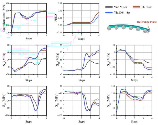
Figure 7.
Stress and strain variations at the centroid of the reference plane during different analysis steps under 30° horizontal bending and 15° vertical bending.
As shown in Figure 6a, in the first analysis step (pre-stretching stage), the maximum equivalent stress in the blank is approximately 282.2 MPa, which is greater than the initial yield stress of 272 MPa. The corresponding contour region includes the reference plane area in Figure 7. Therefore, it can be concluded that after the first analysis step, plastic yielding has occurred at the center of the reference cross-section, which is also reflected in Figure 7, where the equivalent plastic strain starts to deviate from zero. However, the equivalent stress curves of different models coincide at this point. This is because the initial stresses near the yield surface are small, and the differences introduced by the anisotropic models in the calculation of equivalent stress are also minimal. Comparing the different stress components at this stage reveals that their behaviors vary. Among them, S11, S22, and S33 shown in Figure 7 represent the three normal stress components, corresponding to the directions of the global coordinate system in Figure 1. S12, S13, and S23 represent the corresponding shear stress components. For example, the S22 component shows similar curves for all models, while the S11 component exhibits considerable differences. This is due to the differences in stress variations along different directions introduced by the anisotropic models. These differences will lead to variations in the final simulation results, which is the key focus of this study.
After entering the second analysis step, due to the horizontal bending process, the pre-stretched blank is brought closer to the die, and the volume change in the reference point unit is minimal, with only a shape change occurring. As a result, the PEEQ (the equivalent plastic strain) value changes only slightly, and a plateau appears in the curve graph. However, corresponding differences in the equivalent stress and different stress components are observed at this point. This is because the direction of concentrated stress changes as a result of the shape alteration. Under the same level of deformation, stresses in different directions exhibit significant differences due to the material’s plastic anisotropy. Additionally, the anomalous sawtooth fluctuations observed in the S13 stress component in Hill’s 48 model are caused by computational errors during the iterative calculation of partial derivatives. The corresponding curve in the figure shows fluctuations when entering the second analysis step, and no similar changes occur thereafter. Since the fluctuations do not cause any deviations in the final data, the subsequent curve changes follow a similar pattern. Therefore, it is concluded that this error does not affect the final results. Upon entering the vertical bending analysis step, the stress components under different models show significant differences, especially the normal stresses S11, S22, and S33. However, the calculated equivalent stress differences remain small. This is due to the stress distribution differences introduced by the anisotropic models, but the equivalent stress, which represents the overall stress state, does not change significantly. Based on the differences in yield functions, the PEEQ value gradually accumulates as the equivalent strain changes minimally, and thus increases as the deformation progresses. Consequently, after the post-stretching analysis step, this difference is further amplified. At the final analysis step, when the simulation ends, the PEEQ difference between different material models becomes apparent. The PEEQ for the Von Mises model is 1.85 × 10⁻², while for Hill’s 48 model, it is 1.81 × 10⁻², and for Yld2004-18p, it is 1.36 × 10⁻². The error values of the two anisotropic models are 2% and 26.5%, showing significant differences when isotropic simplification is applied. However, the corresponding equivalent stress values are 289.64 MPa, 301.61 MPa, and 295.67 MPa, and the error values are 4.1% and 2.1%, with only minor differences.
Figure 8 compares and analyzes the cross-sectional deformation result contours at 200 mm, including equivalent stress and equivalent strain. By comparing the corresponding indicators in Figure 8a,b, it can be seen that the indicators obtained using the subroutine solution show little difference from those obtained by the software’s built-in solver. The maximum equivalent stresses are 279.2 MPa and 276.2 MPa, respectively, with a negligible error of about 1%. Correspondingly, the error in the maximum equivalent strain is also very small, at approximately 2.6%. Figure 8c,d employ the Hill’s 48 and Yld2004-18p models for the solution, respectively. Different yield models introduce certain errors in equivalent stress and equivalent strain, reaching up to 13% and 27%, respectively. However, there is no intuitive difference in the contour distribution in the corresponding images. This is because, during the deformation process, the differences caused by different yield models only significantly affect local deformation values and have a relatively minor impact on the overall deformation results. After entering the yield state, the growth rate of equivalent stress significantly slows down with the accumulation of deformation (as shown in the stress–strain curve in Figure 3). Therefore, in the equivalent stress contour plot shown in Figure 8, there are large areas of red, while the PEEQ contour plot is evenly distributed.
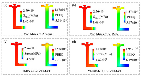
Figure 8.
Stress and strain variations in cross-section. (a) Results of Von Mises model for Abaqus; (b) Results of Von Mises model for VUMAT; (c) Results of Hill’s 48 model for VUMAT; (d) Results of Yld2004-18p model for VUMAT.
3.2. Influence of Material Models on Deformation Results
Based on the above analysis, this study conducted FE simulations of the forming process under different bending angle process parameters. During the deformation result analysis, the PEEQ indicator is typically used to represent the local deformation degree and potential shape errors in the blank. The centerline path of the section is chosen to represent the overall deformation results, as shown in Figure 9. The horizontal axis of the curve represents the distance from the middle of the symmetry plane. From the figure, it is observed that the curves for different material models under different process parameters exhibit local peaks. These peaks are due to differences caused by the discrete die contacting the local areas of the blank. Comparing the different material models, the peak positions correspond well and are located at the blank-die contact area. Additionally, it can be seen that the horizontal bending process has a smaller effect on the PEEQ, whereas the vertical bending process has a larger effect on the PEEQ. This is because, during the horizontal bending process, the blank tends to undergo shape changes with minimal volume change. In contrast, during the vertical bending process, the blank experiences significant volume changes due to tangential forces from the clamps, leading to larger changes in equivalent plastic strain.
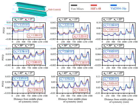
Figure 9.
PEEQ variation curves along Path-Centroid under different bending angle process parameters and error values for different models.
The comparison of different material model curves under various process parameters shows that the Hill’s 48 model aligns closely with the isotropic Von Mises model, exhibiting only minor deviations at peak values. In contrast, the Yld2004-18p model displays notable differences across various positions. To quantify the degree of variation, the peak errors eH and eY between the Hill’s 48 and Yld2004-18p models and the isotropic model were calculated. Across the same process parameters, eH values were slightly lower than eY, in line with the curves shown. However, the differences in eH and eY across different parameters are minimal, and the values for eY are also small, less than 10%. This suggests that an isotropic simplification can effectively capture the overall shape error defects in the deformation process analyzed in this study.
Furthermore, as depicted in Figure 1, during the FSBRD process, significant contact occurs between the flange of the L-shaped profile and the roller dies. This contact results in stress concentrations in the contact area of the flange, as illustrated in Figure 6. Due to the resistance to horizontal and vertical bending provided by the roller dies, maximum deformation typically occurs in the flange area. Thus, PEEQ analysis on the flange is often used to represent deformation due to contact. Figure 10 illustrates the PEEQ variation along the flange path under different bending angle parameters, along with the error values for each material model. Here, errors eH and eY are defined as in the previous sections. Comparing these results with those in Figure 9 for Path-Centroid, it is evident that the PEEQ peak along Path-Flange is significantly higher than that along Path-Centroid, while PEEQ values in non-peak areas remain comparable. This finding confirms that localized contact on the flange induces substantial localized deformation, which macroscopically manifests as local indentations. In non-contact areas, the PEEQ distribution across the cross-section remains uniform.
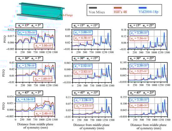
Figure 10.
PEEQ variation curves along Path-Flange under different bending angle process parameters and error values for different models.
For different material models, unlike the Path-Centroid case, the error of the curve is no longer less than 10%, and non-negligible errors emerge. When αH = 15° and αV = 25°, there is an error eY of 3.39 × 10⁻² between the Yld2004-18p material model and the Von Mises isotropic model. The corresponding error rate is as high as 22.6%, which is significantly greater than 10%. Therefore, it is concluded that using the isotropic simplification for the model under these conditions would result in a relatively large error. This is due to the relatively large process parameters and high degree of deformation. As a result, the differences caused by material anisotropy are significant and cannot be ignored. Correspondingly, when αV = 25°, the values of eY under different αH parameters are all relatively large, being 3.39 × 10⁻², 2.59 × 10⁻², and 3.10 × 10⁻², respectively. The corresponding error rates are 22.6%, 19.9%, and 23.2%, all of which are significantly greater than 10%. Similarly, when αH = 45°, the values of eY corresponding to different αV are also relatively large. This indicates that the isotropic simplification cannot be used when the process parameters are relatively large.
In addition, as can be seen from the figure, when αH = 45°, the indicators eY and eH show a significant degree of closeness. For example, when αH = 45° and αV = 15°, the two indicators are 2.28 × 10⁻² and 2.15 × 10⁻², respectively, corresponding to error rates of 22.8% and 21.5%, indicating that the errors are close. Therefore, both the Yld2004-18p material model and the Hill’s 48 material model can describe the process deformation results relatively well. However, when αH = 30° and αV = 25°, the difference between the two indicators becomes larger, being 2.59 × 10⁻² and 5.27 × 10⁻², respectively, with corresponding error rates of 19.9% and 4.1%. This is because, in the process applied in this study, vertical bending induces greater contact deformation. Therefore, compared to horizontal bending deformation, an increase in vertical bending deformation is more likely to reveal differences in anisotropy. As a result, the corresponding eY is larger, and the Yld2004-18p material model provides a more accurate description of the deformation results. An analysis of the computational time for the corresponding finite element simulations reveals significant differences among the material models. The average simulation time using the Von Mises model is approximately 24.49 h. In contrast, the Hill’s 48 model requires about 31.12 h, indicating a notable increase in computational time. The most computationally intensive model is the Yld2004-18p model, which takes as long as 71.86 h. Therefore, when selecting a material model, simplification should be made as much as possible within an acceptable error range to reduce computational costs.
In summary, when the deformation degree is relatively large, an anisotropic material model should be selected for a more accurate description of the process. In other cases, the Von Mises model can be used for simplification. When the vertical bending angle αV is large, there is a significant difference between the Yld2004-18p material model and the Hill’s 48 model. Therefore, the Yld2004-18p material model should be chosen to reduce simulation errors. When the horizontal bending angle αH is large, the difference between the Yld2004-18p and Hill’s 48 models is relatively small. Thus, the Hill’s 48 material model can be selected to reduce both errors and computational time costs.
The difference in results is caused by localized contact. Figure 11 compares the PEEQ results in the localized contact zone of the material models under different deformation levels. As shown in Figure 11a, when the deformation level is small (αH = 15°), the results from the different material models are similar. The maximum abrupt values of local PEEQ for the three models are 4.24 × 10⁻², 4.32 × 10⁻², and 4.63 × 10⁻², respectively, indicating small differences. Compared with the isotropic model, the differences introduced by the two anisotropic models are 1.9% and 9.2%, both less than 10%. Therefore, when the deformation level is small, the error caused by using the isotropic simplification is relatively minor.
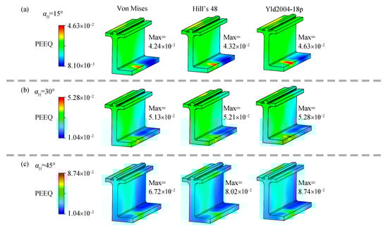
Figure 11.
PEEQ results near the contact area under different parameters. (a) Results when αH = 15°; (b) Results when αH = 30°; (c) Results when αH = 45°.
In Figure 11c, when the deformation degree is relatively large, with αH = 45°, the corresponding PEEQ also shows a significant abrupt change, with local maximum values of 6.72 × 10⁻², 8.02 × 10⁻², and 8.74 × 10⁻², respectively. At this point, noticeable differences appear among the indicators corresponding to different material models. The difference introduced by the Hill’s 48 model is 19.3%, and that by the Yld2004-18p model is 29.6%, both exceeding 15%. Therefore, it is concluded that isotropic simplification of the material model at this stage would introduce significant errors.
3.3. Results of Experimental Analysis
To validate the applicability of the simplified FE model through practical experiments, this paper uses springback as the reference metric. This is because springback is relatively easy to measure in both actual experiments and FE simulations. As previously mentioned, the differences introduced by various material models are mainly manifested at local contact areas with significant deformation. Figure 12a shows that the cross-sectional strain distribution in the non-contact area is uniform, while obvious localized strain jumps occur in the cross-section of the contact area. Figure 12b illustrates how springback is represented in the FE simulation process. The principle of solving springback in bent profiles is based on determining the stress–strain state of the cross-section [21]. Therefore, altering the cross-sectional strain distribution will directly affect the final calculation of springback. This leads to differences in the springback results obtained from simulations using different material models.
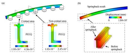
Figure 12.
(a) PEEQ results of contact area and non-contact area; (b) Springback result of the profile.
Simulations and experimental tests were conducted for various horizontal bending angles to validate the FE model and the related theoretical analyses. The forming process and springback measurement process are shown in Figure 13 below. Figure 13b illustrates the process of measuring the springback of L-shaped section profile. During the measurement, the unloaded experimental piece is placed on the equipment. And the bracket and detection point positions of the detection unit are adjusted to match the position of the unloaded formed piece. By comparing it with the position of the forming mold, the required springback amount can be obtained.
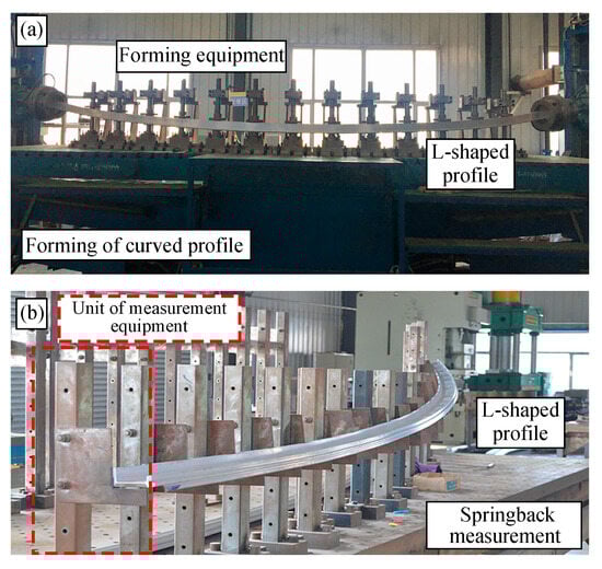
Figure 13.
(a) Forming equipment of L-shaped profile; (b) Springback measurement equipment of L-shaped profile.
As shown in Figure 14, during the FSBRD forming process, the profile blank will exhibit localized indentations due to contact with the discretized roller die. These indentations appear near the contact zones corresponding to the edges of the die, as illustrated in Figure 14b. This matches the FE simulation results shown in Figure 11. The contact between the profile and the roller die alters the stress–strain state of the profile’s cross-section, which in turn affects the springback results. Additionally, since the deformation caused by localized contact is relatively large, it is more significantly influenced by the anisotropic properties of the material. Moreover, as the degree of deformation increases, the constraint exerted by the roller die on the profile blank also increases, leading to a greater influence of the anisotropic properties. This aligns with the variation patterns summarized earlier.
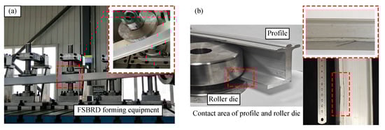
Figure 14.
(a) FSBRD forming process; (b) Contact of profile and roller die during the forming process.
The springback results are measured as shown in Figure 15. It is clear that different material models significantly impact the numerical values of springback. The Yld2004-18p anisotropic model provides results that are closer to the experimental values, thus offering higher accuracy. By comparing the springback values across different process parameters, it can be seen that, at smaller bending angles, the differences between the FE models and experimental results are minimal. This makes the error introduced by the isotropic simplification negligible.
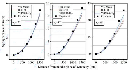
Figure 15.
Springback under different material models and the experimental results with parameter of αV = 15°.
As shown in the figure, when the horizontal bending angle αH = 15°, the simulation results of different material models are close to the experimental results, with relatively small differences. The springback value increases as the reference point moves away from the middle plane of symmetry. At a distance of 1500 mm from the middle plane, the experimental springback is about 5.2 mm. The simulation results from the different material models are 4.67 mm, 4.75 mm, and 4.89 mm, with errors of 10.2%, 8.7%, and 5.9%, respectively, all less than 15%. Since these differences are considered small, it is concluded that the isotropic simplified model can be used for relatively accurate simulation and analysis. However, when αH = 45°, the differences among the different material models become more significant. The errors in the simulation results from the different material models are 25.6%, 21.5%, and 11.6%, respectively. Among them, the Yld2004-18p anisotropic model yields the smallest error, less than 15%. Therefore, this material model should be selected for the analysis, consistent with earlier findings.
Figure 16 compares the springback results under three different deformation levels. When αH = 15° and αV = 5°, the overall deformation during the forming process is relatively small. In this case, the springback curves of the deformation results from the different material models overlap well. Compared with the experimental results, the errors are relatively small, being 7.4%, 6.2%, and 4.1%, respectively. Therefore, under these process parameters, an isotropic model can be used for simulation to improve computational efficiency. When αH = 45° and αV = 25°, the deformation level is higher. By comparing the differences between the three material models and the experimental results, the errors are found to be 19.2%, 16.2%, and 8.9%, respectively. Due to the relatively large errors introduced by the isotropic simplification, the Yld2004-18p material model should be selected for simulation.
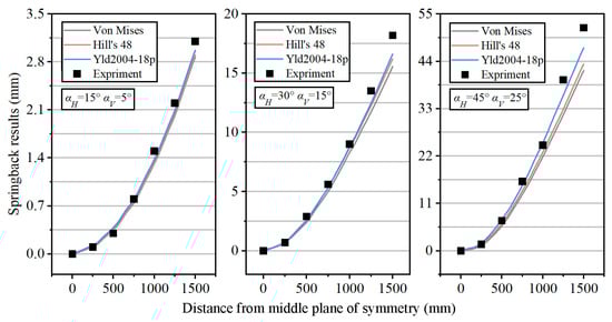
Figure 16.
Springback under different material models and the experimental results with different parameters.
In summary, as the process parameters change, the differences in simulation results among different material models increase with the rise in deformation degree. When conducting related research, model selection should be based on the actual error tolerance requirements. In this study, an error value of 15% is taken as the permissible error threshold. Therefore, when the horizontal bending angle (αH) exceeds 30° and the vertical bending angle (αV) exceeds 15°, the anisotropic Yld2004-18p and Hill’s 48 model should be selected. Otherwise, the isotropic Von Mises model can be used for simplification to improve computational efficiency. Furthermore, when choosing the anisotropic model, the Hill’s 48 model should be prioritized within the allowable error range to enhance computational efficiency.
4. Conclusions
This study conducted finite element simulations of the roller-based flexible three-dimensional stretch-bending process using Al6005A-T6 aluminum alloy profiles with an L-shaped cross-section as the research object. Anisotropic testing was performed to obtain the necessary material properties. The study then conducted finite element simulations based on three material yield models: Von Mises, Hill’s 48, and Yld2004-18p. To implement these models, UMAT/VUMAT user-defined material subroutines were developed. Finally, the FSBRD process was simulated using these models to investigate their performance and accuracy.
The results indicate that, across the different material models, the equivalent stress of the workpiece exhibited minimal variation during deformation. And the differences in equivalent plastic strain also remain minor. However, substantial variations are observed among the different stress components. This is due to the distinct stress flows in each material model, which are influenced by the anisotropy of the materials and affect stress distribution across different directions. Further analysis of equivalent plastic strain under varying process parameters revealed noticeable differences among material models. Yet, the overall deviation values are low, and critical details, such as local peak positions corresponding to discrete contact areas, are clearly captured.
In springback analysis, the differences introduced by varying material models accumulate as deformation increases. This is due to the changes in cross-sectional stress and strain caused by localized contact deformation, which ultimately leads to variations in springback. Consequently, using the isotropic Von Mises model for qualitative analysis is a reasonable choice to enhance computational efficiency. For quantitative analysis of springback results, the isotropic Von Mises model remains viable for rapid computation when deformation levels are low. However, when deformation is significant, the Yld2004-18p model provides a more accurate representation of anisotropy. It significantly reduces the error between FE simulation and experimental results, providing better accuracy for practical applications. For cases with large overall deformation but small local deformation differences, the Hill’s 48 model is preferred. It improves simulation efficiency while considering anisotropy. Based on the research scheme proposed in this paper, the simplified simulation analysis model can be appropriately adjusted according to the actual deformation process and production tolerance requirements during practical application.
Supplementary Materials
The following supporting information can be downloaded at: https://www.mdpi.com/article/10.3390/met15091036/s1, Supporting Information: Program Code.
Author Contributions
Conceptualization: S.Y.; Methodology: Y.L.; Data curation: S.Y. and Y.W. and Y.L.; Software: Y.W. and S.Y.; Investigation: C.L.; Writing—original draft preparation: Y.W. and S.Y.; Writing-review &editing: Y.L. and C.L.; Funding acquisition: C.L.; Literature search: Y.W.; Figures: Y.W. and S.Y.; Visualization: Y.W.; Study design: C.L. and Y.W.; Project administration: C.L. All authors have read and agreed to the published version of the manuscript.
Funding
This work was financially supported by the National Natural Science Foundation of China (No. 52505378) and Jilin Provincial Scientific and Technological Department (20220201048GX).
Data Availability Statement
The original contributions presented in this study are included in the article/Supplementary Materials. Further inquiries can be directed to the corresponding authors.
Conflicts of Interest
The authors declare no competing interests.
References
- Chen, M.H.; Gao, L.; Mao, H.H.; Zuo, D.W.; Wang, M. Numerical simulation of stretch bending process and springback for T section aluminum extrusions. In Advances In Machining & Manufacturing Technology VIII; Yuan, Z.J., Xu, X.P., Zuo, D.W., Yuan, J.L., Yao, Y.X., Eds.; Trans Tech Publications Ltd.: Wollerau, Switzerland, 2006; Volume 315–316, pp. 416–420. [Google Scholar]
- Schilp, H.; Suh, J.; Hoffmann, H. Reduction of springback using simultaneous stretch-bending processes. Int. J. Mater. Form. 2012, 5, 175–180. [Google Scholar] [CrossRef]
- Liang, J.; Chen, C.; Li, Y.; Liang, C. Effect of roller dies on springback law of profile for flexible 3D multi-point stretch bending. Int. J. Adv. Manuf. Technol. 2020, 108, 3765–3777. [Google Scholar] [CrossRef]
- Li, M.Z.; Liu, Y.H.; Su, S.Z.; Li, G.Q. Multi-point forming: A flexible manufacturing method for a 3-d surface sheet. J. Mater. Process. Technol. 1999, 87, 277–280. [Google Scholar] [CrossRef]
- Li, M.Z.; Cai, Z.Y.; Sui, Z.; Yan, Q.G. Multi-point forming technology for sheet metal. J. Mater. Process. Technol. 2002, 129, 333–338. [Google Scholar] [CrossRef]
- Yanagimoto, J.; Banabic, D.; Banu, M.; Madej, L. Simulation of metal forming—Visualization of invisible phenomena in the digital era. CIRP Ann. 2022, 71, 599–622. [Google Scholar] [CrossRef]
- Wang, L.; Luan, X.; Liu, S.; Wang, X. Analysis of wall thickness evolution and forming quality of sheet metal manufactured by wrinkles-free forming method. Int. J. Mater. Form. 2024, 17, 44. [Google Scholar] [CrossRef]
- Vrh, M.; Halilovič, M.; Starman, B.; Štok, B. Modelling of springback in sheet metal forming. Int. J. Mater. Form. 2009, 2, 825–828. [Google Scholar] [CrossRef]
- Liu, Z.; Kumar, D.; Jirathearanat, S.; Wong, W.H. A multiple-tool method for fast FEM simulation of incremental sheet forming process. Int. J. Adv. Manuf. Technol. 2023, 128, 4311–4329. [Google Scholar] [CrossRef]
- Lee, M.-G.; Kim, S.-J. Elastic-plastic constitutive model for accurate springback prediction in hot press sheet forming. Met. Mater. Int. 2012, 18, 425–432. [Google Scholar] [CrossRef]
- Li, X.C.; Yang, Y.Y.; Wang, Y.Z.; Bao, J.; Li, S.P. Effect of the material-hardening mode on the springback simulation accuracy of V-free bending. J. Mater. Process. Technol. 2002, 123, 209–211. [Google Scholar] [CrossRef]
- Zeng, D.; Xia, Z.C. A modified Mroz model for springback prediction. J. Mater. Eng. Perform. 2007, 16, 293–300. [Google Scholar] [CrossRef]
- Chen, K.; Lin, J.; Wang, L. Influence of mechanical properties of AHSS on springback in sheet forming. Steel Res. Int. 2010, 81, 813–816. [Google Scholar]
- N’Jock, M.Y.; Badreddine, H.; Labergere, C.; Yue, Z.; Saanouni, K.; Dang, V.T. An application of fully coupled ductile damage model considering induced anisotropies on springback prediction of advanced high strength steel materials. Int. J. Mater. Form. 2021, 14, 739–752. [Google Scholar] [CrossRef]
- Ma, J.; Welo, T.; Wan, D. The impact of thermo-mechanical processing routes on product quality in integrated aluminium tube bending process. J. Manuf. Process. 2021, 67, 503–512. [Google Scholar] [CrossRef]
- Liao, J.; Xue, X.; Lee, M.-G.; Barlat, F.; Gracio, J. On twist springback prediction of asymmetric tube in rotary draw bending with different constitutive models. Int. J. Mech. Sci. 2014, 89, 311–322. [Google Scholar] [CrossRef]
- Esmaeilpour, R.; Kim, H.; Park, T.; Pourboghrat, F.; Mohammed, B. Comparison of 3D yield functions for finite element simulation of single point incremental forming (SPIF) of aluminum 7075. Int. J. Mech. Sci. 2017, 133, 544–554. [Google Scholar] [CrossRef]
- Rong, H.; Ying, L.; Hu, P.; Hou, W. Characterization on the thermal anisotropic behaviors of high strength AA7075 alloy with the Yld2004-18p yield function. J. Alloys Compd. 2021, 877, 159955. [Google Scholar] [CrossRef]
- Barlat, F.; Aretz, H.; Yoon, J.W.; Karabin, M.E.; Brem, J.C.; Dick, R.E. Linear transfomation-based anisotropic yield functions. Int. J. Plast. 2005, 21, 1009–1039. [Google Scholar] [CrossRef]
- Abedrabbo, N.; Pourboghrat, F.; Carsley, J. Forming of aluminum alloys at elevated temperatures—Part 2: Numerical modeling and experimental verification. Int. J. Plast. 2006, 22, 342–373. [Google Scholar] [CrossRef]
- Ma, J.; Welo, T. Analytical springback assessment in flexible stretch bending of complex shapes. Int. J. Mach. Tools Manuf. 2021, 160, 103653. [Google Scholar] [CrossRef]


Disclaimer/Publisher’s Note: The statements, opinions and data contained in all publications are solely those of the individual author(s) and contributor(s) and not of MDPI and/or the editor(s). MDPI and/or the editor(s) disclaim responsibility for any injury to people or property resulting from any ideas, methods, instructions or products referred to in the content. |
© 2025 by the authors. Licensee MDPI, Basel, Switzerland. This article is an open access article distributed under the terms and conditions of the Creative Commons Attribution (CC BY) license (https://creativecommons.org/licenses/by/4.0/).