Prediction Modeling and Parameter Optimization for Robotic Belt Grinding 42CrMo Steel Using Response Surface Methodology and Grey Relational Analysis

Abstract

To address high-precision robotic abrasive belt grinding of 42CrMo steel, this study adopted the orthogonal central composite design with grinding force, feed rate, and rotational speed as key parameters, establishing and verifying regression models for material removal depth (MRD) and surface roughness (Ra). Results showed that the models’ relative errors are within 6% (MRD) and 10% (Ra). Grinding force and feed rate exert a strong coupling effect on MRD, while feed rate–rotational speed and grinding force–feed rate interactions significantly influence Ra, with “saddle-shaped” response surfaces. Grey relational analysis determined the optimal parameters: 75 N grinding force, 22.4 mm·s⁻¹ feed rate, and 3261 rpm rotational speed, achieving a maximum MRD of 1.975 mm and a minimum Ra of 3.506 μm. The tolerance range of the optimal parameters is F = 70–80 N, v_f = 20–24 mm·s⁻¹, and ω = 3000–3500 rpm. This research provides robust support for process parameter prediction and optimization in high-precision robotic abrasive belt grinding of 42CrMo steel.

1. Introduction

42CrMo medium-carbon alloy steel possesses prominent characteristics of high strength, excellent toughness, and superior wear resistance. Consequently, it has been extensively applied in the production of annular parts, such as gears [1], bolts [2], crankshafts [3], and bearings [4].

Currently, research on the grinding of 42CrMo steel is predominantly focused on grinding wheels, and many scholars have conducted investigations on the optimization of process parameters [5,6]. Kwak et al. [7] analyzed grinding power and surface roughness during the external cylindrical grinding of quenched SCM440 steel (similar to 42CrMo). They found that increasing cutting depth has a more significant effect on the maximum height of surface roughness than on the centerline average height. Based on grinding parameters, they established a quadratic response surface model for grinding power and surface roughness via the response surface methodology (RSM). Hou et al. [8] found that grooved grinding wheels enhance the undeformed chip thickness (UCT) of 42CrMo steel, reduce specific plowing and sliding energy, and consequently improve workpiece grinding quality. Zaghal et al. [9] deduced the influence patterns of polishing speed, feed rate, and polishing force on the residual stress and microhardness of 42CrMo4 steel, and identified the optimal polishing process parameters. Roy et al. [10] employed RSM to examine how parameters like grinding wheel speed, workpiece speed, and cross-feed speed affect the grinding contact temperature and material removal rate of 42CrMo steel, ultimately determining the optimal input parameters. Wang et al. [11] also adopted RSM to investigate the influence of grinding parameters on the surface roughness of 42CrMo steel. The results showed that the surface roughness increases with cutting depth and workpiece feed rate, while grinding linear speed has no significant effect.

However, 42CrMo steel has high density and poor thermal conductivity. A large amount of grinding heat is easily generated during grinding, causing the workpiece surface layer to rapidly reach the austenitizing temperature in a short time, which induces phase-transformation hardening or uncontrollable softening [12]. In contrast, abrasive belt grinding offers the advantages of elastic contact and cold-state grinding [13,14], which can significantly reduce grinding heat and workpiece hardening, thereby facilitating improvements in grinding quality.

Li et al. [15] converted the surface roughness and material removal rate of 45# steel into a comprehensive objective using the weighted objective method. By integrating central composite design and response surface analysis, they obtained the optimal values of abrasive grain size, contact force, abrasive belt linear speed, and feed rate for abrasive belt grinding. Zhang et al. [16] proposed a material removal model for robotic abrasive belt grinding based on energy conversion during the grinding process, and concluded that normal contact force is the most prominent grinding parameter affecting material removal depth (MRD). Ren et al. [17] examined the impacts of grinding parameters on material removal, grinding heat, and surface quality from both macroscopic and microscopic perspectives. The results showed that an increase in theoretical grinding depth can improve material removal efficiency and grinding temperature while enhancing surface quality, and its influence is more significant than that of abrasive belt speed. Shang et al. [18] studied the effects of abrasive belt grinding parameters on the surface roughness of TC4 alloy. They found that surface roughness is most sensitive to abrasive grain size, followed by grinding force, and least sensitive to abrasive belt linear speed. The optimal parameter range was determined as follows: abrasive belt grain size of 120#–150#, linear speed of 15–20 m·s⁻¹, and grinding force of 10–15 N. Within this range, surface roughness can be controlled within 0.57 μm. Pan et al. [19] investigated the influence of five process parameters—grinding speed, table feed rate, grinding depth, deflection angle, and tilt angle—on workpiece surface roughness. Their findings revealed that surface roughness decreases as grinding speed increases, increases with higher feed rates, and exhibits significant fluctuations with changes in grinding depth.

Notably, with the in-depth application of intelligent algorithms in the manufacturing field, recent research on robotic abrasive belt grinding has focused more on improving machining accuracy and state control capabilities through intelligent predictive models. Tao et al. [20] proposed a predictive model based on UCT and a generalized regression neural network (GRNN). Experimental validation demonstrated that the model’s predicted values are highly consistent with experimental results, offering distinct advantages over traditional models. Jia et al. [21] developed an MRD prediction model for blades using the adaptive neuro-fuzzy inference system (ANFIS). This model exhibits a mean absolute percentage error of merely 3.976%, outperforming alternatives such as random forest, artificial neural network, and support vector regression models. Chen et al. [22] proposed a model predictive control method based on a deep belief network (DBN), which can accurately predict the sudden changes in grinding state induced by deformation. Surindra et al. [23] conducted a study on abrasive belt state monitoring based on machine learning. By comparing algorithms including k-nearest neighbor, support vector machine, multi-layer perceptron, and decision tree, they found that decision tree and random forest models optimized by hyperparameters have the highest average test accuracy, and decision tree and random forest models have the lowest delay.

Nevertheless, abrasive belt grinding is a nonlinear process involving the coupling of multiple factors [24]. Due to the elastic contact between the abrasive belt and the workpiece, as well as the hardening phenomenon of 42CrMo steel, it is relatively difficult to accurately predict MRD during the grinding process [25,26].

A comprehensive review of the previous studies reveals that research on 42CrMo steel grinding primarily focuses on wheel grinding and conventional abrasive belt grinding. In contrast, insufficient attention has been devoted to robotic abrasive belt grinding technology. Although some studies [27] have attempted to predict MRD in robotic grinding, two core gaps remain unresolved:

First, there is a lack of modeling for parameter coupling effects. In robotic abrasive belt grinding, the elastic contact between the abrasive belt and workpiece induces strong nonlinear coupling among grinding force, feed rate, and rotational speed. However, existing models [16] largely simplify these interactive effects, leading to low prediction accuracy for both MRD and Ra. Second, there is a deficiency in dual-objective optimization that accounts for uncertainties in practical engineering scenarios. Most studies [17] only optimize a single objective—either MRD or Ra—failing to balance processing efficiency and quality. Even in the few multi-objective optimization studies [28], the discreteness of experimental data and parameter tolerances in industrial scenarios are not considered. This renders the “optimal parameters” only applicable to ideal laboratory conditions, lacking fault tolerance and practicality for engineering applications.

Thus, in this study, grinding experiments on 42CrMo steel were performed using an Adaptive Triangular abrasive Belt (ATB) tool (Shanghai Saiwider Robot Co., Ltd., Shanghai, China) and an industrial robot. Focusing on three key grinding parameters of grinding force, feed rate, and rotational speed, the Orthogonal Central Composite Design (OCCD) method was employed to design the experiments. Concurrently, the response surface regression analysis method was utilized to develop predictive models for MRD and surface roughness Ra. Subsequently, response surfaces were leveraged to conduct an in-depth analysis of the interactive effects of grinding process parameters on MRD and Ra. Finally, with the maximum MRD and minimum Ra as dual objectives, the Grey Relational Analysis (GRA) method was applied to optimize the grinding parameters, ultimately yielding their optimal combination.

2. Materials and Methods

2.1. Experimental Materials and Setup

The material employed in this experiment was annealed 42CrMo steel, which was pre-machined into experimental specimens with dimensions of 300 mm × 100 mm × 30 mm. The experimental setup, as shown in Figure 1, comprised a KUKA KR210 industrial robot (KUKA Robotics China Co., Ltd., Shanghai, China) and an ATB tool. The ATB tool was mounted on the sixth axis of the KR210 robot, with the feed rate regulated by the robot itself. Key parameters of the ATB tool were as follows: the rotational speed was adjustable within the range of 2000–6000 rpm with an accuracy of 1 rpm; the grinding force was adjustable from 5 to 120 N with an accuracy of 1 N. The abrasive belt is a 984F-type ceramic alumina abrasive belt manufactured by 3M Company (Shanghai, China).

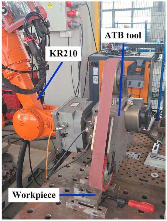
Figure 1. The experimental setup for robotic belt grinding 42CrMo steel.

2.2. Experimental Method

Owing to the rapid initial wear of the abrasive belt, each new abrasive belt was pre-ground six times to reach the stable wear stage, which was defined as the initial state of the abrasive belt to ensure the accuracy of experimental data. Subsequently, each abrasive belt was replaced with a new one after 24 grinding tests. During the tests, after six grinding times, an electronic balance with an accuracy of 0.1 g was employed to measure the removal mass of the 42CrMo steel specimen. The MRD was thereafter calculated using Equation (1).

$$D_{\mathrm{MR}}={\displaystyle \frac{1000M}{N\rho lb}}$$

(1)

where $D_{\mathrm{MR}}$ represents the material removal depth, namely MRD [mm]; M denotes the removal weight [g]; N is the tested number, with N = 6; ρ is the density of 42CrMo steel, with ρ = 7.56 g·cm⁻³; and l and b represent the cross-sectional length and width of the specimen, respectively, with l = 300 mm and b = 30 mm.

A stylus-type surface roughness tester (Model: JITAI810, Jiahe Precision Instrument, Shenzhen, China) was employed to measure the surface roughness Ra of the specimens. The JITAI810 tester features a measurement range of 0.005–16.000 μm and an indication accuracy of 0.001 μm. The measuring stylus is a diamond tip, with a cone angle of 90° and a tip radius of 5 μm. During measurements, the speed was maintained at 1 mm·s⁻¹. The sampling length was set to 2.5 mm, while the measurement length (also termed evaluation length) was 10 mm, which is exactly four times the sampling length.

Five Ra measurement points were set at 50 mm intervals along the length direction of the specimen. At each point, Ra was measured along the centerline of the specimen’s width, yielding 5 data per experiment. For the MRD measurement, each experiment was also tested five times. For the original data of MRD and Ra, Grubb’s test was adopted (confidence level: 95%, corresponding critical value G_0.05,5 = 1.672) to eliminate outliers. The average value of the remaining valid data, along with the standard deviation σ, was used as the final result.

Based on previous experimental results [29], an 80-grit abrasive belt was employed, and the grinding process parameters for 42CrMo steel were selected as follows: grinding force F = 40–80 N, feed rate v_f = 5–25 mm·s⁻¹, and rotational speed ω = 3000–5000 rpm. Accounting for the interaction effects and quadratic effects among factors, the grinding experiments for 42CrMo steel were designed via the OCCD method [15]. The adoption of OCCD is primarily based on three considerations: first, it leverages orthogonality to simplify experimental points, substantially reducing the number of experiments and improving efficiency; second, it enables accurate separation of the main effects and interaction effects among grinding force, feed rate, and rotational speed, which aligns with the research demand for analyzing parameter coupling relationships; third, its experimental points conform to the actual industrial grinding parameter range, avoiding the extreme values that may arise in Rotatable CCD and thus enhancing engineering practicability.

The factor level coding for the grinding experiments is presented in Table 1. Here, the number of influencing factors is three, the number of zero-level tests is three, and the distance between the axial point and the center point was calculated as 1.353.

Table 1. Factor and level coding for 42CrMo steel grinding experiments.

Factors	Levels
	−1.353	−1	0	1	1.353
Grinding force, F [N]	40	45	60	75	80
Rotational speed, ω [rpm]	3000	3261	4000	4739	5000
Feed rate, vf [mm·s−1]	5	7.6	15	22.4	25

Based on the factor level coding, the experimental scheme was designed using Design Expert 13.0 software. The experimental response variables were MRD (marked as variable of D_MR) and surface roughness Ra, and the experimental scheme is presented in Table 2. For clarity, the experimental response results are also presented in Table 2.

Table 2. Experimental scheme and results for 42CrMo steel grinding.

No.	Factors			DMR ± σ [mm]	Ra ± σ [μm]
	F	ω	vf
1	−1	−1	−1	0.595 ± 0.031	4.429 ± 0.149
2	1	−1	−1	1.128 ± 0.052	4.361 ± 0.128
3	−1	1	−1	0.183 ± 0.028	4.194 ± 0.117
4	1	1	−1	0.298 ± 0.036	3.682 ± 0.082
5	−1	−1	1	1.048 ± 0.04	3.883 ± 0.103
6	1	−1	1	1.975 ± 0.042	3.506 ± 0.102
7	−1	1	1	0.302 ± 0.035	4.753 ± 0.131
8	1	1	1	0.564 ± 0.045	4.022 ± 0.087
9	−1.353	0	0	0.217 ± 0.033	4.975 ± 0.163
10	1.353	0	0	0.698 ± 0.056	4.164 ± 0.143
11	0	−1.353	0	1.997 ± 0.048	3.706 ± 0.125
12	0	1.353	0	0.304 ± 0.057	4.108 ± 0.136
13	0	0	−1.353	0.239 ± 0.026	4.496 ± 0.126
14	0	0	1.353	0.536 ± 0.037	4.102 ± 0.117
15	0	0	0	0.381 ± 0.041	4.427 ± 0.151
16	0	0	0	0.365 ± 0.034	4.519 ± 0.105
17	0	0	0	0.458 ± 0.037	4.325 ± 0.141

3. Results and Discussion

3.1. Regression Model Establishment

The second-order model is a widely used regression model in RSM, serving to approximate the relationship between input variables and response variables. Its mathematical expression typically takes the form of a quadratic polynomial [28]:

$$Y={\beta }_0+{\displaystyle \sum _i^k{\beta }_i{x}_i}+{\displaystyle \sum _{i=1}^{k-1}{\displaystyle \sum _{j=i+1}^k{\beta }_{ii}{x}_i{x}_j}}+{\displaystyle \sum _{j=1}^k{\beta }_{ij}}{x}_i^2+{\epsilon }_q$$

(2)

where $x_i$ denotes the input variables; $Y$ is the response variable; ${\beta }_0$ is the intercept term; ${\beta }_i$, ${\beta }_{ii}$, and ${\beta }_{ij}$ are the regression coefficients of the linear terms, interaction terms, and quadratic terms, respectively; ${\epsilon }_q$ is the error term; and k is the number of input variables.

Using the 17 sets of experimental results from Table 2, regression coefficients were derived using Equation (2). Subsequently, full second-order regression equations were established for the MRD and surface roughness Ra of 42CrMo steel, respectively, with respect to grinding force, feed rate, and rotational speed.

$$\begin{array}{ll}{D}_{\mathrm{MR}}=& -0.706040+0.006631F-0.118803v_{\mathrm{f}}+0.000702\omega \\ & -0.001220F\cdot v_{\mathrm{f}}+6.10059\times {10}^{-6}F\cdot \omega -0.000021v_{\mathrm{f}}\cdot \omega \\ & +0.000013F^2+0.006690{v_{\mathrm{f}}}^2-6.39694\times {10}^{-8}{\omega }^2\end{array}$$

(3)

$$\begin{array}{ll}\mathrm{Ra}=& 3.82759-0.011904F+0.020772v_{\mathrm{f}}+0.000722\omega \\ & -0.000899F\cdot v_{\mathrm{f}}-5.95399\times {10}^{-6}F\cdot \omega +0.000053v_{\mathrm{f}}\cdot \omega \\ & +0.000277F^2-0.005512{v_{\mathrm{f}}}^2-1.59182\times {10}^{-7}{\omega }^2\end{array}$$

(4)

where $D_{\mathrm{MR}}$ and Ra are the MRD and surface roughness of 42CrMo steel, respectively.

Analysis of variance (ANOVA) was performed for Equations (3) and (4), with the results presented in Table 3 and Table 4, respectively. Among the key statistical metrics, the F-value is used to compare variances, testing for significant differences between groups and evaluating the overall significance of regression models. The p-value is employed to assess the significance of test results, and assists in determining whether to reject the null hypothesis. If the p-value is less than a predetermined significance level (α = 0.05 in this study), the null hypothesis is rejected, and it is concluded that the regression model or grinding parameter is statistically significant.

Table 3. ANOVA results for material removal depth D_MR of 42CrMo steel.

Source	Sum of Squares	df	Mean Square	F-Value	p-Value	Note
Model	4.9600	9	0.5506	25.11	0.0002	significant
F	0.5315	1	0.5315	24.24	0.0017
vf	2.8700	1	2.8700	126.57	<0.0001
ω	0.3734	1	0.3734	17.03	0.0044
F·vf	0.1466	1	0.1466	6.69	0.0362
F·ω	0.0366	1	0.0366	1.67	0.2375
vf·ω	0.1047	1	0.1047	4.77	0.0652
$F^2$	0.0001	1	0.0001	0.0025	0.9614
$v_{\mathrm{f}}^2$	0.9789	1	0.9789	44.64	0.0003
${\omega }^2$	0.0082	1	0.0082	0.3732	0.5606
Residual	0.1535	7	0.0219	—	—
Lack-of-fit	0.1486	5	0.0297	12.02	0.0786	not significant
Pure error	0.0049	2	0.0025	—	—
Cor total	5.11	16	—	—	—

R² = 0.9700; Adjusted R² = 0.9313. Adequate precision = 16.34 > 4 indicates it has an adequate signal.

Table 4. ANOVA results for surface roughness Ra of 42CrMo steel.

Source	Sum of Squares	df	Mean Square	F-Value	p-Value	Note
Model	2.3000	9	0.2557	21.77	0.0003	significant
F	0.6637	1	0.6637	56.52	0.0001
vf	0.0885	1	0.0885	7.53	0.0287
ω	0.0919	1	0.0919	7.82	0.0266
F·vf	0.0796	1	0.0796	6.78	0.0352
F·ω	0.0348	1	0.0348	2.97	0.1286
vf·ω	0.6612	1	0.6612	56.31	0.0001
$F^2$	0.0251	1	0.0251	2.14	0.1872
$v_{\mathrm{f}}^2$	0.6088	1	0.6088	51.85	0.0002
${\omega }^2$	0.0507	1	0.0507	4.31	0.0764
Residual	0.0882	7	0.0117	—	—
Lack-of-fit	0.0634	5	0.0127	1.35	0.4783	not significant
Pure error	0.0188	2	0.0094	—	—
Cor total	2.38	16	—	—	—

R² = 0.9655; Adjusted R² = 0.9212. Adequate precision = 17.16 > 4 indicates it has an adequate signal.

As can be seen from Table 3 and Table 4, the p-values for the significance tests of both D_MR and Ra models are less than 0.05, indicating that both models are significant.

The feed rate exerts the most significant influence on MRD, whereas the rotational speed has the least impact. In contrast, the grinding force is the dominant factor affecting Ra, while the feed rate shows the minimal effect.

For the D_MR model, the coefficient of determination R² is 0.97, a value close to 1, which indicates that the model has a good fitting degree. Similarly, the Ra model achieves an R² of 0.9655, also demonstrating strong fitting performance. Meanwhile, the p-values of the lack-of-fit terms for models are greater than 0.05, indicating that the lack-of-fit is not significant. This result further validates the reliability of two models, as they do not deviate significantly from the actual relationships embedded in the experimental data.

Adequate precision is a key metric for evaluating the signal-to-noise ratio. Ideally, a value greater than 4 is considered indicative of sufficient signals. For the D_MR and Ra models, the adequate precision values are 16.34 and 17.16, respectively—both well above the threshold of 4. This confirms that the models possess adequate capacity to distinguish the effects of different experimental factors on the response values. Consequently, they are highly reliable for predicting MRD and Ra.

Additionally, Table 3 reveals that the p-values of the interaction terms ($F\cdot \omega$ and $v_{\mathrm{f}}\cdot \omega$) and quadratic terms ($F$ and ${\omega }^2$) are all greater than 0.05. This indicates that their impacts on the D_MR model are non-significant, and they can all be neglected. Table 4 further demonstrates that, for the Ra model, the p-value of the interaction term $v_{\mathrm{f}}\cdot \omega$ is substantially larger than those of $v_{\mathrm{f}}$ and $\omega$ alone. This confirms that the interaction between feed rate and rotational speed exerts a strong influence on Ra, yielding a “1 + 1 > 2” synergistic effect. Across both models, the p-value of the quadratic term $v_{\mathrm{f}}^2$ is extremely small. This highlights that the quadratic term of feed rate plays a crucial role in influencing MRD and Ra.

To further simplify the full regression model while ensuring accuracy, non-significant terms identified in the significance analysis (i.e., terms with a p-value > 0.05) were eliminated. The full second-order response surface models were subsequently revised, and the simplified regression equations for MRD and Ra are as follows:

$$\begin{array}{ll}{D}_{\mathrm{MR}}& =0.039485 + 0.032592F-0.202464v_{\mathrm{f}} + 0.000242\omega \\ & \hspace{0.17em}-0.001220F\cdot v_{\mathrm{f}} +0.006990{v_{\mathrm{f}}}^2\end{array}$$

(5)

$$\begin{array}{c}\mathrm{Ra}=6.79173-0.002497F+0.020411v_{\mathrm{f} }-0.000909\omega \\ \hspace{0.33em}\hspace{1em}\hspace{0.33em}\hspace{0.33em}-0.000899F\cdot v_{\mathrm{f}}+0.000053v_{\mathrm{f}}\cdot \omega -0.005500{v_{\mathrm{f}}}^2\end{array}$$

(6)

Table 5 presents the fitting statistics and model comparison statistics for a comparative analysis between the simplified regression models (5)–(6) and the full regression models (3)–(4).

Table 5. Fitting statistics and model comparison statistics for original and simplified models.

Model	R2		Adjusted R2		Predicted R2		PRESS
	Full	Simplified	Full	Simplified	Full	Simplified	Full	Simplified
DMR	0.9700	0.9407	0.9313	0.9137	0.9162	0.9065	1.2300	0.9373
Ra	0.9655	0.9294	0.9212	0.9071	0.8954	0.8824	0.5900	0.5353

As is evident from the statistical results in Table 5, due to the elimination of nonsignificant parameter terms in the simplified models, both their adjusted R² show a slight decrease compared with the full models. Nevertheless, all indicators still stably remain within the “good or higher” fitting range, indicating that the core fitting capability of the models has not been substantially compromised.

In terms of generalization performance, the predicted R² of the simplified models only undergoes a minimal decline. This implies that their predictive ability for new data is highly comparable to that of the full models, with no significant loss in generalization performance—they can still reliably capture the core correlative relationships between grinding parameters and response variables.

Notably, the Predicted Residual Sum of Squares (PRESS) of the simplified models is lower than that of the full models. This indicates that after removing redundant parameters, the simplified models yield smaller prediction errors and higher prediction accuracy.

In summary, the simplified models achieve parameter simplification through the systematic elimination of nonsignificant terms. While significantly reducing model complexity, they not only further enhance the prediction accuracy for MRD and Ra, but also constrain losses in fitting goodness and generalization ability within a controllable range. By balancing scientific rigor and practical utility, these simplified models are expected to serve as an efficient and reliable tool for the rapid prediction and optimization of parameters in practical grinding processes.

To validate the accuracy of the simplified regression models, grinding experiments on 42CrMo steel experimental specimens were conducted under different grinding parameters. The experimentally measured results were compared with those predicted by the regression models, as presented in Table 6.

Table 6. Experimental validation results of simplified regression models for D_MR and Ra.

No.	F [N]	ω [rpm]	vf [mm·s−1]	DMR [mm]		Relative Error [%]	Ra [μm]		Relative Error [%]
				Measured	Predicted		Measured	Predicted
1	40	5000	25	0.606	0.640	5.6	4.597	4.946	7.6
2	45	5000	5	1.534	1.604	4.6	3.552	3.222	−9.3
3	50	4000	5	1.458	1.495	2.5	4.101	3.831	−6.6
4	55	5000	25	0.701	0.672	−4.1	4.171	4.571	9.6
5	60	4500	15	0.498	0.522	4.8	4.213	4.388	4.2
6	65	3000	5	1.657	1.650	−0.4	4.659	4.370	−6.2
7	70	4000	10	1.068	1.109	3.8	3.985	4.126	8.6
8	75	3500	10	1.025	1.063	3.4	3.972	4.258	7.2
9	50	4500	10	0.801	0.822	2.6	4.503	4.166	−7.5
10	65	4500	20	0.427	0.408	−4.4	4.235	4.348	2.7
11	70	4500	20	0.435	0.449	3.2	3.987	4.246	6.5
12	70	3500	10	1.048	0.988	−5.7	4.529	4.315	−4.7
13	40	3000	5	0.935	0.978	4.6	4.472	4.545	1.6
14	40	3000	25	0.162	0.156	−3.7	4.507	4.114	−8.7
15	40	5000	5	1.397	1.472	5.4	3.398	3.257	−4.1
16	40	5000	25	0.632	0.640	1.3	4.776	4.946	3.6
17	80	3000	25	0.253	0.240	−5.1	3.440	3.115	−9.4
18	80	5000	25	0.711	0.724	1.8	4.021	3.947	−1.8

As indicated in Table 6, the maximum relative error between the predicted and measured D_MR is 5.7%, demonstrating that the established prediction model for MRD is highly accurate. For the Ra model, the maximum relative error is 9.6%. Although its accuracy is marginally lower than that of the D_MR model, it still falls within the acceptable error range.

In summary, the D_MR regression model exhibits an error within 6%, and the Ra regression model shows an error within 10%. Both models yield valid prediction results within the scope of the experimental process parameters.

3.2. Response Surface Analysis for Material Removal Depth

Based on the RSM method, response surfaces for any two variables can be established. This enables intuitive observation of the influence of variable parameters on response outputs. Figure 2 presents the response surface, depicting the effect of grinding process parameters on MRD.

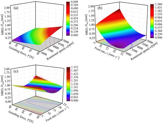
Figure 2. Response surfaces for the interactive effects of grinding process parameters on MRD of 42CrMo steel: (a) grinding force and rotational speed, (b) feed rate and rotational speed, (c) grinding force and feed rate.

As observed in Figure 2a, at a constant grinding force, the MRD of 42CrMo steel increases with the elevation of rotational speed. This is attributed to the fact that higher rotational speed results in more grinding cycles of abrasive grains in the same area per unit time, leading to a more thorough grinding effect and consequently an increased MRD. When the rotational speed is fixed, MRD rises with the increase in grinding force. During the robotic abrasive belt grinding process, the grinding force F acts directly on 42CrMo steel. As the grinding force increases, the average load borne by each abrasive grain per unit time increases correspondingly. This not only deepens the cutting depth of abrasive grains into the specimen but also increases the number of abrasive grains participating in grinding. With more abrasive grains exerting a cutting effect, the material removal efficiency is enhanced, thereby increasing the MRD.

The response surface in Figure 2a exhibits an approximately linear relationship, which indicates that the interaction between grinding force and rotational speed is weak. This further justifies the elimination of their interaction term during the establishment of the D_MR regression model.

In fact, based on the previous research [27], the following relationship holds between MRD and the grinding process parameters:

$$D_{\mathrm{MR}}=K{\displaystyle \frac{v_{\mathrm{s}}+v_{\mathrm{f}}}{v_{\mathrm{f}}}}{\displaystyle \frac{{F_{\mathrm{n}}}^{\raisebox{1ex}{$5$}\!\left/ \!\raisebox{-1ex}{$3$}\right.}}{H_{\mathrm{v}}\tan \frac{\theta }{2}}}{\displaystyle {\int }_{3\sigma -m+{\delta }_{\max }}^{3\sigma }\frac{1}{\sqrt{2\pi }\sigma }{e}^{-\frac{h^2}{2{\sigma }^2}}\mathrm{d}h}$$

(7)

where $v_{\mathrm{s}}$ is the tangential velocity of the abrasive belt at the 42CrMo steel surface with $v_{\mathrm{s}}=2\pi R\omega$, F_n is the normal force, H_v is the Vickers hardness of the ground surface of 42CrMo steel specimen, $\theta$ is the protrusion angle of the abrasive grains, K is a coefficient, m is the maximum penetration depth, ${\delta }_{\max }$ is the maximum elastic deformation of the 42CrMo steel specimen, σ is the standard deviation of the abrasive grain protrusion height h, and the distances from the highest and lowest abrasive grains to the average abrasive grain height follow a 3σ distribution.

It can be inferred from Equation (7) that the MRD increases linearly with the tangential velocity $v_{\mathrm{s}}$. Specifically, as the rotational speed n increases, the tangential velocity $v_{\mathrm{s}}$ rises accordingly, which in turn leads to an increase in MRD. Equation (7) also reveals that MRD is proportional to the normal force F_n, because F_n is proportional to the grinding force F. Specifically, an increase in F will result in a corresponding increase in F_n. Consequently, the MRD increases with the elevation of the grinding force F.

The response surface presented in Figure 2b exhibits a “smooth single-inclined surface” morphology. This indicates that the interaction between rotational speed and feed rate on MRD is significantly stronger than that between grinding force and rotational speed, as illustrated in Figure 2a. This conclusion is further corroborated by the p-values presented in Table 3.

In Figure 2b, when the rotational speed is held constant, the MRD decreases with increasing feed rate. Initially, the MRD drops sharply; however, once it exceeds a certain threshold, the rate of reduction slows significantly, and the MRD even stops decreasing. This phenomenon can be explained as follows. In abrasive belt grinding, material is deformed into chips under the extrusion and friction of abrasive grain cutting edges, forming the machined surface. Microscopically, a single abrasive grain’s cutting process involves three stages: sliding, plowing, and cutting [30,31]. As feed rate increases, the residence time of each single abrasive grain in the grinding zone shortens, reducing the number of grains penetrating the specimen surface. This weakens the grinding effect and leads to a gradual decrease in MRD. When feed rate reaches a specific value, the abrasive grains can no longer sufficiently penetrate the specimen surface, only inducing sliding and plowing. This leads to insufficient grinding, with MRD dropping to the minimum. Beyond this point, further increases in feed rate have a negligible impact on MRD. This trend is also consistent with Equation (7), which indicates that the MRD of 42CrMo steel specimens decreases as the feed rate increases.

Additionally, 42CrMo steel undergoes work hardening during grinding [32,33], with the degree of work hardening dependent on feed rate. At relatively low feed rates, abrasive grains remain in the grinding zone longer, leading to more grains participating in grinding. This results in a higher degree of work hardening and increases surface Vickers hardness H_v. As the feed rate increases, fewer abrasive grains are involved in grinding, work hardening is weakened, and H_v decreases. According to Equation (7), MRD increases as H_v decreases, which mitigates the reduction in MRD caused by higher feed rate. Therefore, considering the combined effects of effective grinding abrasive grains and surface Vickers hardness, MRD does not decrease linearly with increasing feed rate. Instead, MRD drops rapidly at relatively low feed rates, while the rate of decrease slows considerably at relatively high feed rates.

As shown in Figure 2c, the response surface illustrating the combined effect of grinding force and feed rate on MRD exhibits a hyperbolic paraboloid (also called as “inverted saddle surface”) morphology. For different combinations of grinding force and feed rate, MRD exhibits a complex bidirectional variation trend, namely, along the direction of a single parameter (either grinding force or feed rate), MRD does not simply increase or decrease, but follows a pattern integrating both “concave” and “convex” characteristics. This highlights the key regulatory role of feed rate in the MRD-F relationship, and confirms a significant interaction between these two parameters. Thus, grinding force and feed rate exhibit strong coupling—they do not affect MRD independently but jointly determine it.

As discussed earlier, feed rate influences the surface Vickers hardness of 42CrMo steel, which in turn affects MRD. Similarly, grinding force also alters the specimen’s surface H_v. As grinding force increases, the specimen’s plastic deformation intensifies, and both grinding temperature and heat rise [34]. Under the combined action of plastic deformation and grinding heat, the specimen undergoes work hardening, leading to corresponding changes in surface hardness. At relatively low grinding forces, plastic deformation dominates, and surface hardness increases with the rise in grinding force. When the grinding force further increases, grinding heat gradually becomes the dominant factor, and it mitigates the specimen’s work hardening, slowing or even reversing the increase in surface hardness. Additionally, according to Equation (7), $D_{\mathrm{MR}}\propto {\displaystyle \frac{F_{\mathrm{n}}}{v_{\mathrm{f}}\cdot H_{\mathrm{v}}}}$. Therefore, under the coupled effect of feed rate and grinding force, MRD is jointly determined by these two parameters and the surface hardness they induce, ultimately resulting in the “inverted saddle surface” morphology.

3.3. Response Surface Analysis for Surface Roughness

Figure 3 presents the response surfaces illustrating the effect of grinding process parameters on the surface roughness Ra of 42CrMo steel.

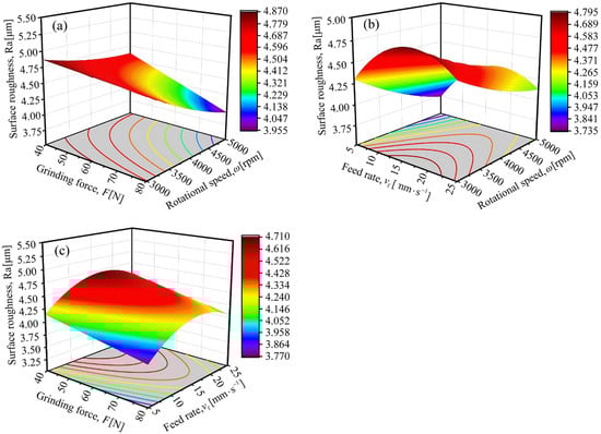
Figure 3. Response surfaces for the interactive effects of grinding process parameters on the surface roughness Ra of 42CrMo steel: (a) grinding force and rotational speed, (b) feed rate and rotational speed, (c) grinding force and feed rate.

It can be observed from Figure 3a that the response surface of grinding force and rotational speed resembles an inclined plane. The coupling effect between these two parameters is weak, and their interactive influence on surface roughness Ra is relatively minor. When grinding force is held constant, Ra tends to decrease with increasing rotational speed. Similarly, when the rotational speed is fixed, Ra also decreases as grinding force increases.

As shown in Figure 3b,c, the response surfaces of “feed rate—rotational speed” and “grinding force—feed rate” both exhibit a “saddle surface” morphology. This indicates that their interaction significantly influences Ra. When the rotational speed or grinding force is held constant, Ra first increases and then decreases with rising feed rate, peaking at 15 mm·s⁻¹. When feed rate is fixed, Ra generally shows a gradual downward trend with the increase in rotational speed or grinding force.

Surface roughness is essentially caused by the irregular topography formed by abrasive grains during material removal [26]. For specimens with an initial surface roughness of ${\mathrm{Ra}}^{\Theta }$, their surface peaks are gradually flattened by the cutting action of abrasive grains during grinding, resulting in a gradual reduction in Ra. Once the surface peaks are fully removed, subsequent grinding creates new surface irregularities, which causes the surface roughness to increase. This phase is defined as the over-grinding stage. According to existing studies [35,36], the evolution model of Ra can be expressed as follows:

$$\left\{\begin{array}{ll}\mathrm{Ra}={\mathrm{Ra}}^{\Theta }-k_a{\displaystyle \frac{F}{H_{\mathrm{v}}{v}_{\mathrm{f}}}}\left[{\displaystyle \frac{\sqrt{r^2-y^2}\cdot r}{2}}+{\displaystyle \frac{y^2}{2}}\ln \left({\displaystyle \frac{r}{y}}\right)\right]& (\mathrm{a})\\ \mathrm{Ra}=k_a{\displaystyle \frac{F}{H_{\mathrm{v}}{v}_{\mathrm{f}}}}\left[{\displaystyle \frac{\sqrt{r^2-y^2}\cdot r}{2}}+{\displaystyle \frac{y^2}{2}}\ln \left({\displaystyle \frac{r}{y}}\right)\right]-{\mathrm{Ra}}^{\Theta }& (\mathrm{b})\end{array}\right.$$

(8)

where $k_a$ is a constant coefficient for a specific abrasive belt.

From Equation (8), before the 42CrMo steel enters the over-grinding stage, its surface roughness Ra decreases with increasing grinding force and rotational speed, which explains the Ra variation trend with these two parameters observed in Figure 3a. It follows that when grinding force and rotational speed increase simultaneously, Ra decreases rapidly, which aligns with Figure 3a. As feed rate increases, Ra rises accordingly, peaking at 15 mm·s⁻¹. Beyond this threshold, further increasing feed rate induces the 42CrMo steel to enter the over-grinding stage, and Ra begins to decrease in line with Equation (8b)—consistent with the response surfaces in Figure 3b,c.

4. Optimization for Grinding Process Parameters

4.1. Grey Relational Analysis for Grinding Parameters

When simultaneous optimization of MRD and Ra is required, GRA can effectively address this multi-objective optimization problem. It exhibits unique advantages, especially in nonlinear systems with small sample sizes and incomplete information, as it does not require assuming data distribution characteristics or predefining a weight assignment model. Additionally, GRA features a concise calculation process and can effectively quantify the correlation strength between grinding parameters and the dual objectives [37,38]. In this study, a total of 17 sets of valid experimental data were obtained using OCCD experiments, with a relatively limited sample size and the presence of parameter coupling effects. Therefore, GRA, which is more compatible with the experimental design scale of this study, was selected as the optimization tool. The specific implementation process involves three key steps:

Firstly, standardize the original experimental data. In abrasive belt grinding, MRD directly reflects grinding efficiency, and a higher MRD is desirable. Thus, the original MRD data is standardized using Equation (9).

$${D^{\prime }}_{\mathrm{MR}\text{\_}i}\left(k\right)={\displaystyle \frac{D_{\mathrm{MR}\text{\_}i}\left(k\right)-\min \left[D_{\mathrm{MR}\text{\_}i}\left(k\right)\right]}{\max \left[D_{\mathrm{MR}\text{\_}i}\left(k\right)\right]-\min \left[D_{\mathrm{MR}\text{\_}i}\left(k\right)\right]}}$$

(9)

where ${D^{\prime }}_{\mathrm{MR}\text{\_}i}\left(k\right)$ represents the dimensionless standardized MRD, and $D_{\mathrm{MR}\text{\_}i}\left(k\right)$ denotes the original MRD, mm.

Ra characterizes the grinding quality of 42CrMo steel surface, and a smaller Ra is theoretically preferable. Thus, the original Ra data are standardized using Equation (10).

$${\mathrm{R}\mathrm{a}}_i^{\prime }\left(k\right)={\displaystyle \frac{\max \left[{\mathrm{Ra}}_i\left(k\right)\right]-{\mathrm{Ra}}_i\left(k\right)}{\max \left[{\mathrm{Ra}}_i\left(k\right)\right]-\min \left[{\mathrm{Ra}}_i\left(k\right)\right]}}$$

(10)

where ${\mathrm{R}\mathrm{a}}_i^{\prime }\left(k\right)$ denotes the dimensionless standardized surface roughness, and ${\mathrm{Ra}}_i\left(k\right)$ represents the original surface roughness, μm.

Secondly, the deviation sequences of MRD and Ra are calculated using Equation (11):

$$\left\{\begin{array}{l}{\Delta }_i\left(D_{\mathrm{MR}}\right)=\left|{\mathrm{X}}_0\left(k\right)-{D^{\prime }}_{\mathrm{MR}\_i}\left(k\right)\right|\hfill \\ {\Delta }_i\left(\mathrm{Ra}\right)=\left|{\mathrm{X}}_0\left(k\right)-{\mathrm{R}\mathrm{a}}_i^{\prime }\left(k\right)\right|\hfill \end{array}\right.$$

(11)

where ${\mathrm{X}}_0\left(k\right)$ represents the value of ideal solution. In this study, the reference sequence for all responses is set to ${\mathrm{X}}_0\left(k\right)$ = 1.

Finally, calculate the grey relational coefficients and grey relational grades. The grey relational grade denotes the correlation between two sequences. Specifically, it reflects the closeness of the relationship between each factor within the system and the reference factor. A higher grade indicates a stronger correlation and a more significant influence of the factor on the system. The formula for the grey relational coefficient ${\zeta }_i\left(s\right)$ of the s-th parameter in the i-th experiment is as follows:

$${\zeta }_i\left(s\right)={\displaystyle \frac{\min \left[{\Delta }_i\left(s\right)\right]+\lambda \cdot \max \left[{\Delta }_i\left(s\right)\right]}{{\Delta }_i\left(s\right)+\lambda \cdot \max \left[{\Delta }_i\left(s\right)\right]}}$$

(12)

where ${\zeta }_i\left(s\right)$ represents the deviation sequence of the s-th parameter with ${\Delta }_i\left(s\right)={\Delta }_i\left(D_{\mathrm{MR}}\right)$ or ${\Delta }_i\left(s\right)={\Delta }_i\left(\mathrm{Ra}\right)$, $\lambda$ denotes the deviation coefficient with a range from 0 to 1. Its value is adjusted according to the actual system, and a smaller $\lambda$ indicates a larger deviation. In this study, all factors are considered equally important, so $\lambda$ = 0.5.

The grey relational grade ${\gamma }_i$ is the average of grey relational coefficients, calculated as follows:

$${\gamma }_i={\displaystyle \frac{1}{p}}{\displaystyle \sum _{s=1}^p{\zeta }_i\left(s\right)}$$

(13)

where p denotes the number of optimization objectives, p = 2.

Using the above method, GRA was performed on the two objective parameters of D_MR and Ra, presented in Table 2. The results are shown in Table 7.

Table 7. Calculation results of grey relational grade for dual-objective optimization of D_MR and Ra of 42CrMo Steel.

Group	Comparison Sequence		Deviation Sequence		Grey Relational Coefficient		Grey Relational $\mathbf{Grade}, {\mathit{\gamma }}_{\mathit{i}}$
	${{\mathit{D}}^{\prime }}_{\mathbf{MR}\text{\_}\mathit{i}}\left(\mathit{k}\right)$	${\mathrm{R}\mathrm{a}}_i^{\prime }\left(\mathit{k}\right)$	${\mathbf{\Delta }}_{\mathit{i}}\left({\mathit{D}}_{\mathbf{MR}}\right)$	${\mathbf{\Delta }}_{\mathit{i}}\left(\mathbf{Ra}\right)$	${\mathit{\zeta }}_{\mathit{i}}\left({\mathit{D}}_{\mathbf{MR}}\right)$	${\mathit{\zeta }}_{\mathit{i}}\left(\mathbf{Ra}\right)$
1	0.227	0.372	0.773	0.628	0.393	0.443	0.418
2	0.521	0.418	0.479	0.582	0.511	0.462	0.487
3	0	0.532	1.000	0.468	0.333	0.517	0.425
4	0.063	0.880	0.937	0.120	0.348	0.806	0.577
5	0.477	0.743	0.523	0.257	0.489	0.661	0.575
6	0.988	1.000	0.012	0	0.977	1.000	0.989
7	0.066	0.151	0.934	0.849	0.349	0.371	0.360
8	0.210	0.649	0.790	0.351	0.388	0.588	0.488
9	0.019	0	0.981	1.000	0.338	0.333	0.336
10	0.284	0.552	0.716	0.448	0.411	0.527	0.469
11	1.000	0.864	0	0.136	1.000	0.786	0.893
12	0.067	0.590	0.933	0.410	0.349	0.549	0.449
13	0.031	0.326	0.969	0.674	0.340	0.426	0.383
14	0.195	0.594	0.805	0.406	0.383	0.552	0.468
15	0.109	0.373	0.891	0.627	0.359	0.444	0.402
16	0.100	0.310	0.900	0.690	0.357	0.420	0.389
17	0.152	0.442	0.848	0.558	0.371	0.473	0.422

As is evident from Table 7, Group 6 has the highest grey relational grade of 0.989, which can simultaneously meet the requirements of maximizing MRD and minimizing Ra. Its optimal grinding parameters are as follows: grinding force: 75 N, feed rate: 22.4 mm·s⁻¹, and rotational speed: 3261 rpm. Under these parameter settings, the maximum MRD reaches 1.975 mm and the minimum Ra is 3.506 μm. In contrast, group 11 has the second-highest grey relational grade of 0.893. Under the parameters of this group, an MRD of 1.997 mm and a Ra of 3.706 μm can be achieved, which are very close to those of Group 6.

4.2. Uncertainty and Tolerance Analysis for the Optimal Grinding Parameter Solution

Data of the top four groups (including the optimal group and the top three sub-optimal groups) in terms of grey relational grade in Table 7 are presented in Table 8.

Table 8. Data and confidence interval calculation results of the top four groups by grey relational grade.

Group	${\mathit{\gamma }}_{\mathit{i}}$	F [N]	ω [rpm]	vf [mm·s−1]	DMR ± σ [mm]	Ra ± σ [μm]	Ci
							DMR [mm]	Ra [μm]
6	0.989	75	3261	22.4	1.975 ± 0.042	3.506 ± 0.122	1.923–2.027	3.355–3.657
11	0.893	60	3000	15	1.997 ± 0.048	3.706 ± 0.125	1.937–2.057	3.551–3.861
4	0.577	75	4739	5	0.298 ± 0.036	3.682 ± 0.082	0.256–0.340	3.580–3.784
5	0.575	45	3261	22.4	1.048 ± 0.040	3.883 ± 0.103	0.998–1.098	3.755–4.011

For the data in Table 8, the confidence intervals of D_MR and Ra can be calculated, respectively, using Equation (14), based on the t-distribution.

$$C_i=\overline{x}\pm t_{\alpha /2, \mathrm{d}f}\cdot {\displaystyle \frac{\sigma }{\sqrt{n}}}$$

(14)

where $C_i$ denotes the confidence intervals of D_MR and Ra, $\overline{x}$ represents the mean value of the measured data, $\sigma$ is the standard deviation, df stands for the degrees of freedom, $\alpha$ indicates the confidence level, and n is the sample size of each experimental group.

In this study, a 95% confidence level (i.e., $\alpha$ = 0.05) was adopted for outlier elimination via Grubb’s test. Given the small sample size (n = 5), the degrees of freedom were calculated as df = 4, yielding a critical value of t_0.05/2,4 = 2.776 for the t-distribution. The confidence intervals of MRD and Ra, calculated using the data from Table 8, are also listed in the table.

As indicated in Table 8, the confidence interval of D_MR for the optimal group (D_MR = 1.975 mm) overlaps with that of the sub-optimal group (D_MR = 1.997 mm). Similarly, the confidence interval of Ra for the optimal group (Ra = 3.506 μm) overlaps with that of the sub-optimal group (Ra = 3.706 μm). This demonstrates that the differences between the two groups lie within the range of statistical uncertainty, implying that the slight numerical discrepancies between the optimal and sub-optimal groups have no practical engineering significance.

Considering the “fluctuation of experimental data” and “industrial application requirements”, the tolerance for the optimal solution was determined, and the fluctuation range of optimal grinding parameters was further derived. 42CrMo steel is primarily utilized for ring-shaped components such as gears and crankshafts, where the surface roughness Ra for medium-precision ground surfaces typically ranges from 3.2 to 6.3 μm. In this study, the optimal Ra (3.506 μm) falls at the lower end of this range; thus, the upper limit of engineering allowable tolerance for Ra was set to 4.0 μm—meaning any fluctuated Ra ≤ 4.0 μm can satisfy application requirements. Using the response surface analysis discussed previously, parameter ranges meeting the criteria of “Ra ≤ 4.0 μm and D_MR ≥ 1.8 mm” (90% of the optimal D_MR) were obtained by fixing two parameters at their optimal values and adjusting the third. The results are presented in Table 9.

Table 9. Tolerance ranges of optimal parameters derived via back-calculation combined with response surface analysis.

Optimized Parameter	Optimal Value	Tolerance Range	Basis (Response Surface Characteristics)
Grinding force, F [N]	75	70–80	When F < 70 N, DMR drops below 1.8 mm; when F > 80 N, Ra exceeds 4.0 μm (Figure 2c)
Feed rate, vf [mm·s−1]	22.4	20–24	When vf < 20 mm·s−1, DMR shows no significant improvement; when vf > 24 mm·s−1, Ra rises sharply to above 4.2 μm (Figure 2b)
Rotational speed, ω [rpm]	3261	3000–3500	When ω < 3000 rpm, Ra increases to 3.9 μm (close to the upper tolerance limit); when ω > 3500 rpm, DMR shows no significant improvement but energy consumption increases (Figure 2a)

Three supplementary experiments within the parameter tolerance range were conducted to further verify that D_MR and Ra still satisfy the requirements of “Ra ≤ 4.0 μm and D_MR ≥ 1.8 mm”. The verification results are presented as follows:

• V1: F = 70 N, v_f = 20 mm·s⁻¹, ω = 3000 rpm → D_MR = 1.82 mm, Ra = 3.85 μm;
• V2: F = 80 N, v_f = 24 mm·s⁻¹, ω = 500 rpm → D_MR = 1.95 mm, Ra = 3.98 μm;
• V3: F = 75 N, v_f = 22.4 mm·s⁻¹, ω = 3261 rpm (optimal value) → D_MR = 1.975 mm, Ra = 3.506 μm (reference value).

Therefore, the tolerance ranges of the optimal grinding parameters are determined as F = 70–80 N, v_f = 20–24 mm·s⁻¹, and ω = 3000–3500 rpm. Parameter combinations within this range can balance grinding efficiency (D_MR) and quality (Ra), and are compatible with the practical needs of robot parameter fine-tuning in industrial production. This avoids the issue of frequent robot parameter calibration when strictly adopting the unique optimal value (75 N, 22.4 mm·s⁻¹, 3261 rpm) in industrial settings.

5. Conclusions

This study investigates the effects of key grinding parameters—including grinding force, rotational speed, and feed rate—on the grinding performance of 42CrMo steel during robotic abrasive belt grinding. The key conclusions are as follows:

(1) Through OCCD experiment, regression models for MRD and Ra were established. ANOVA confirmed that the models have good fitting accuracy, with relative errors within 6% (MRD) and 10% (Ra), respectively. These models can directly serve as practical grinding—allowing technicians to quickly predict MRD and Ra without repeated trials, thereby reducing trial-and-error costs in robotic grinding for 42CrMo steel.

(2) Grinding force and feed rate exhibit a strong coupling effect on MRD, with their response surface presenting an inverted saddle shape. In contrast, grinding force and rotational speed show an approximately linear profile, indicating no significant interaction between them. For Ra, the “feed rate–rotational speed” and “grinding force–feed rate” interactions are significant, with saddle-shaped response surfaces. These findings provide clear guidance for on-site parameter adjustment: when pursuing efficient MRD, priority should be given to optimizing the matching relationship of grinding force and feed rate.

(3) GRA was adopted to achieve the dual-objective optimization of maximizing MRD and minimizing Ra. The optimal parameters were determined as 75 N grinding force, 22.4 mm·s⁻¹ feed rate, and 3261 rpm rotational speed. Under these parameters, the maximum MRD reaches 1.975 mm and the minimum Ra is 3.506 μm. The tolerance range of the optimal grinding parameters is F = 70–80 N, v_f = 20–24 mm·s⁻¹, and ω = 3000–3500 rpm. These parameter combinations within this range balance grinding efficiency and quality, eliminating the need for frequent robot parameter calibration in industrial settings that arises from strictly adopting the singular optimal values (75 N, 22.4 mm·s⁻¹, 3261 rpm).

This study provides basic theoretical and technical support for the high-precision robotic abrasive belt grinding of 42CrMo steel. It lays a foundation for subsequent grinding parameter adjustment. However, this study has certain limitations: the scope of abrasive belt grits and grinding parameters is relatively narrow; dynamic factors in actual production (e.g., robot motion errors and abrasive belt wear rate variations) are not fully considered; the analysis of grinding mechanisms lacks integration of microstructural changes; and only GRA is used for dual-objective optimization.

Accordingly, future research can focus on the following aspects: (1) expanding the research scope by including different abrasive belt grits (e.g., 36#, 60#, 120#) and wider grinding parameter ranges to improve the universality of the research results; (2) introducing online monitoring technologies (e.g., vibration sensors, vision sensors) to real-time track robot end vibration and abrasive belt wear status, and integrate machine learning algorithms (e.g., BP neural network, random forest, XGBoost) to establish a dynamic prediction model for grinding effects; (3) combining scanning electron microscopy (SEM) and other characterization techniques to analyze the surface micro-morphology and microstructure of ground workpieces, clarifying the correlation between micro-grinding mechanisms and macro-performance, and providing more precise theoretical support for parameter optimization; and (4) exploring multi-objective optimization algorithms with higher efficiency (e.g., non-dominated sorting genetic algorithm, NSGA-III) to balance multiple performance indicators and meet the diversified requirements of engineering applications.

References

- Yu, Z.W.; Xu, X.L. Failure investigation of a truck diesel engine gear train consisting of crankshaft and camshaft gears. Eng. Fail. Anal. 2010, 17, 537–545. [Google Scholar] [CrossRef]
- Guo, H.F.; Yan, J.W.; Zhang, R.; He, Z.H.; Zhao, Z.Q.; Qu, T.; Wan, M.; Liu, J.S.; Li, C.D. Failure analysis on 42CrMo steel bolt fracture. Adv. Mater. Sci. Eng. 2019, 2019, 2382759. [Google Scholar] [CrossRef]
- Wang, Y.P.; Luo, Y.C.; Mo, Q.Y.; Huang, B.; Wang, S.Y.; Mao, X.F.; Zhou, L. Failure analysis and improvement of a 42CrMo crankshaft for a heavy-duty truck. Eng. Fail. Anal. 2023, 153, 107567. [Google Scholar] [CrossRef]
- Li, Y.T.; Ju, L.; Qi, H.P.; Zhang, F.; Chen, G.Z.; Wang, M.L. Technology and experiments of 42CrMo bearing ring forming based on casting ring blank. Chin. J. Mech. Eng. 2014, 27, 418–427. [Google Scholar] [CrossRef]
- Hoier, P.; Santhosh, D.K.; Hryha, E.; Krajnik, P. An investigation into the grindability of additively manufactured 42CrMo4 steel. CIRP Ann.-Manuf. Techn. 2024, 73, 257–260. [Google Scholar] [CrossRef]
- Li, N.; Chen, Y.; Kong, D.D. Wear mechanism analysis and its effects on the cutting performance of PCBN inserts during turning of hardened 42CrMo. Int. J. Precis. Eng. Man. 2018, 19, 1355–1368. [Google Scholar] [CrossRef]
- Kwak, J.S.; Sim, S.B.; Jeong, Y.D. An analysis of grinding power and surface roughness in external cylindrical grinding of hardened SCM440 steel using the response surface method. Int. J. Mach. Tool. Manu. 2006, 46, 304–312. [Google Scholar] [CrossRef]
- Hou, Z.; Zhang, X.; Yao, Z. Investigation of cutting mechanism and residual stress state with grooved grinding wheels. Int. J. Adv. Manuf. Tech. 2023, 128, 1455–1471. [Google Scholar] [CrossRef]
- Zaghal, J.; Molnar, V.; Benke, M. Improving surface integrity by optimizing slide diamond burnishing parameters after hard turning of 42CrMo4 steel. Int. J. Adv. Manuf. Tech. 2023, 128, 2087–2103. [Google Scholar] [CrossRef]
- Roy, R.; Ghosh, S.K.; Kaisar, T.; Ahmed, T.; Hossain, S.; Aslam, M.; Kaseem, M.; Rahman, M.M. Multi-response optimization of surface grinding process parameters of AISI 4140 alloy steel using response surface methodology and desirability function under dry and wet conditions. Coatings 2022, 12, 104. [Google Scholar] [CrossRef]
- Wang, C.Y.; Wang, G.C.; Shen, C.E. Analysis and prediction of grind-hardening surface roughness based on response surface methodology-BP neural network. Appl. Sci. 2022, 12, 12680. [Google Scholar] [CrossRef]
- Wang, Y.S.; Xiu, S.C.; Zhang, S.N. Controlling grain sizes of 42CrMo steel by pre-stress hardening grinding. Materials 2019, 12, 3124. [Google Scholar] [CrossRef]
- Zhang, W.; Gong, Y.D.; Sun, Y.; Zhao, J.B. Evaluation of abrasive belt grinding performance in nickel-based superalloy robot grinding. Mater. Manuf. Process. 2024, 39, 1260–1267. [Google Scholar] [CrossRef]
- Liu, Y.; Song, S.Y.; Xiao, G.J.; Huang, Y.; Zhou, K. A high-precision prediction model for surface topography of abrasive belt grinding considering elastic contact. Int. J. Adv. Manuf. Tech. 2023, 125, 777–792. [Google Scholar] [CrossRef]
- Li, F.P.; Xue, Y.; Zhang, Z.Y.; Song, W.L.; Xiang, J.W. Optimization of grinding parameters for the workpiece surface and material removal rate in the belt grinding process for polishing and deburring of 45 steel. Appl. Sci. 2020, 10, 6314. [Google Scholar] [CrossRef]
- Zhang, W.J.; Gong, Y.D.; Xu, Y.C.; Zhao, X.L.; Liang, C.Y.; Yin, G.Q.; Zhao, J.B. Modeling of material removal depth in robot abrasive belt grinding based on energy conversion. J. Manuf. Process. 2023, 97, 76–86. [Google Scholar] [CrossRef]
- Ren, L.J.; Wang, N.N.; Zhang, G.P.; Wang, X.H.; Li, X.T. Comprehensive analysis of the effects of different parameters on the grinding performance for surfaces. Int. J. Adv. Manuf. Tech. 2024, 130, 5147–5164. [Google Scholar] [CrossRef]
- Shang, Y.R.; Hu, S.B.; Qiao, H. Sensitivity study of surface roughness process parameters in belt grinding titanium alloys. Metals 2023, 13, 1825. [Google Scholar] [CrossRef]
- Pan, S.; Ma, L.J.; Yu, X.Q.; Shan, Q. Study on the influence of vibration characteristics on surface roughness in quick-point grinding and prediction model. Int. J. Adv. Manuf. Tech. 2023, 129, 2385–2398. [Google Scholar] [CrossRef]
- Tao, Z.; Li, S.; Zhang, L.; Zhang, D. Surface roughness prediction in robotic belt grinding based on the undeformed chip thickness model and GRNN method. Int. J. Adv. Manuf. Tech. 2022, 120, 6287–6299. [Google Scholar] [CrossRef]
- Jia, H.; Lu, X.; Cai, D.; Xiang, Y.; Chen, J.; Bao, C. Predictive modeling and analysis of material removal characteristics for robotic belt grinding of complex blade. Appl. Sci. 2023, 13, 4248. [Google Scholar] [CrossRef]
- Chen, S.; Zhang, T.; Zou, Y.; Xiao, M. Model Predictive control of robotic grinding based on deep belief network. Complexity 2019, 2019, 1891365. [Google Scholar] [CrossRef]
- Surindra, M.D.; Alfarisy, G.A.F.; Caesarendra, W.; Petra, M.I.; Prasetyo, T.; Tjahjowidodo, T.; Królczyk, G.M.; Glowacz, A.; Gupta, M.K. Use of machine learning models in condition monitoring of abrasive belt in robotic arm grinding process. J. Intell. Manuf. 2025, 36, 3345–3358. [Google Scholar] [CrossRef]
- Zhang, Y.D.; Xiao, G.J.; Gao, H.; Zhu, B.; Huang, Y.; Li, W. Roughness prediction and performance analysis of data-driven superalloy belt grinding. Front. Mater. 2022, 9, 765401. [Google Scholar] [CrossRef]
- Ren, L.J.; Wang, N.A.; Wang, X.H.; Li, X.T.; Li, Y.C.; Zhang, G.P.; Lei, X.Q. Modeling and analysis of material removal depth contour for curved-surfaces abrasive belt grinding. J. Mater. Process. Tech. 2023, 316, 117945. [Google Scholar] [CrossRef]
- Xiao, G.J.; Gao, H.; Zhang, Y.D.; Zhu, B.; Huang, Y. An intelligent parameters optimization method of titanium alloy belt grinding considering machining efficiency and surface quality. Int. J. Adv. Manuf. Tech. 2023, 125, 513–527. [Google Scholar] [CrossRef]
- Shi, D.Q.; Xu, Y.E.; Wang, X.H.; Zhang, H.J. Influence of grinding parameters on the removal depth of 42crmo steel and its prediction in robot electro-hydraulic-actuated abrasive belt grinding. J. Manuf. Mater. Proc. 2025, 9, 76. [Google Scholar] [CrossRef]
- Krajnik, P.; Kopac, J.; Sluga, A. Design of grinding factors based on response surface methodology. J. Mater. Process. Tech. 2005, 162, 629–636. [Google Scholar] [CrossRef]
- Chen, G.; Yang, J.Z.; Yao, K.W.; Xiang, H.; Liu, H. Robotic abrasive belt grinding with consistent quality under normal force variations. Int. J. Adv. Manuf. Tech. 2023, 125, 3539–3549. [Google Scholar] [CrossRef]
- Hokkirigawa, K.; Kato, K. An experimental and theoretical investigation of ploughing, cutting and wedge formation during abrasive wear. Tribol. Int. 1988, 21, 51–57. [Google Scholar] [CrossRef]
- Chen, X.; Opoz, T.T.; Oluwajobi, A. Analysis of grinding surface creation by single-grit approach. J. Manuf. Sci. Eng. 2017, 139, 121007. [Google Scholar] [CrossRef]
- Guo, Y.; Liu, M.H.; Yan, Y.T. Hardness prediction of grind-hardening layer based on integrated approach of finite element and cellular automata. Materials 2021, 14, 5651. [Google Scholar] [CrossRef]
- Zhang, Y.; Ge, P.Q.; Be, W.B. The study for variable grinding depth to control plane grind-hardening layer depth distribution. Int. J. Adv. Manuf. Tech. 2016, 84, 1269–1276. [Google Scholar] [CrossRef]
- Ding, H.H.; Yang, J.Y.; Wang, W.J.; Liu, Q.Y.; Guo, J.; Zhou, Z.R. Wear mechanisms of abrasive wheel for rail facing grinding. Wear 2022, 504–505, 204421. [Google Scholar] [CrossRef]
- Shi, D.Q.; Zeng, X.Y.W.; Wang, X.H.; Zhang, H.J. Parameter optimization and surface roughness prediction for the robotic adaptive hydraulic polishing of NAK80 mold steel. Processes 2025, 13, 991. [Google Scholar] [CrossRef]
- Li, D.W.; Yang, J.X.; Ding, H. Process optimization of robotic grinding to guarantee material removal accuracy and surface quality simultaneously. J. Manuf. Sci. Eng. 2024, 146, 051005. [Google Scholar] [CrossRef]
- Manimaran, G.; Kumar, M.P. Multiresponse optimization of grinding AISI 316 stainless steel using grey relational analysis. Mater. Manuf. Process. 2013, 28, 418–423. [Google Scholar] [CrossRef]
- Zhang, L.Z. Optimization of grinding process parameters for slender tubes through orthogonal experiments and grey relational analysis. Adv. Mech. Eng. 2025, 17, 16878132251358317. [Google Scholar] [CrossRef]
Disclaimer/Publisher’s Note: The statements, opinions and data contained in all publications are solely those of the individual author(s) and contributor(s) and not of MDPI and/or the editor(s). MDPI and/or the editor(s) disclaim responsibility for any injury to people or property resulting from any ideas, methods, instructions or products referred to in the content. |
© 2025 by the authors. Licensee MDPI, Basel, Switzerland. This article is an open access article distributed under the terms and conditions of the Creative Commons Attribution (CC BY) license (https://creativecommons.org/licenses/by/4.0/).