Abstract
In the aerospace field, Ti–Al alloy thin-walled parts, such as blades, generally undergo a large amount of material removal and have a low processing efficiency. Scheduling the feed rate during machining can significantly improve machining efficiency. However, existing feed-rate scheduling methods rarely consider the influence of machining deformation factors and cannot be applied in the finishing stages of thin-walled parts. This study proposes an offline feed-rate scheduling method based on a local stiffness estimation model that can be used to reduce machining errors and improve efficiency in the finishing stage of thin-walled parts. In the proposed method, a predictive model that can rapidly calculate the local stiffness at each cutter location point and a cutting-force prediction model that considers the effect of cutting angle are established. Based on the above model, an offline feed-rate scheduling method that considers machining deformation error constraints is introduced. Finally, an experiment is performed by taking the finishing of actual blade parts as an example. The experimental results demonstrate that the proposed feed-rate scheduling method can improve the machining efficiency of parts while ensuring machining accuracy. The proposed method can also be conveniently applied to feed-rate scheduling in the finishing stage of other thin-walled parts without being limited by machine tools.
1. Introduction
The machining process is very time-consuming for Ti–Al alloy thin-walled parts, such as blades, because of the large amount of material removed. Moreover, because there are regions with low local rigidity in thin-walled parts, large machining deformations are easily produced, resulting in a high scrap rate and difficult machining. Therefore, workers typically choose relatively conservative machining parameters to ensure machining accuracy. This results in time-consuming machining. Scheduling the feed rate in the machining process and using variable feed-rate machining instead of a fixed feed rate can significantly improve machining efficiency.
Feed-rate scheduling is also known as feed-rate optimization. It is a machining program modification process that does not change the machining track of the part but adjusts the feed rate at different positions as required. Several researchers have studied feed-rate scheduling methods [1]. Feed-rate scheduling methods can be divided into two categories according to their execution in real time: online and offline feed-rate scheduling methods.
1.1. Online Feed-Rate Scheduling Method
The online feed-rate scheduling method requires the use of sensors to monitor the machining status and simultaneously adjusts the feed rate online in real time through the actuator according to the optimization algorithm. Adams et al. [2] proposed a feed-rate closed-loop control strategy based on online monitoring of the milling force. Han et al. [3] determined the relationship between feed rate, cutting force, and workpiece deformation through a simulation. During the experiment, the cutting process was monitored in real time using a cutting-force sensor. Based on their proposed blade deformation prediction model and real-time feed-rate optimization algorithm, blade deformation could be controlled within the tolerance range. However, these online methods required the use of cutting-force sensors and open CNC controllers. This generally leads to high application costs for the online method, and its application is not widespread.
1.2. Offline Feed-Rate Scheduling Method
The offline feed-rate scheduling method optimizes the offline machining program by establishing a simulation model of the machining state before the actual machining. This is an active optimization system. It is not limited by the type of machine tool, structure of parts, etc. Compared with the online method, it is more flexible and has a wider range of applications. According to the different control parameters used, offline feed-rate scheduling methods can be divided into methods based on the material removal rate (MRR), cutting force, cutting power, and geometric and kinematic constraints.
1.2.1. MRR-Based Feed-Rate Optimization
The MRR-based method assumes that the work performed by removing the material is proportional to its volume. Therefore, in cases in which other machining parameters except the feed rate are constant, the feed rate is proportional to the instantaneous cutting rate. Jang et al. [4] developed a voxel-based multi-axis CNC machining simulator. They used the number of removed voxels to calculate the MRR and adaptively adjusted the feed rate to improve the machining efficiency. Similarly, Layegh et al. [5] used the commercial solid modeler Parasolid to establish a meshing model of the tool and part and used it for estimating the cutting force. They proposed a feed-rate scheduling method based on an improved force model. This method maintains the predicted cutting force below a predetermined threshold by controlling the feed rate. The MRR can be easily calculated using Boolean operations of the tool and part models. Therefore, this method has been applied to some commercial CAM software. Woo et al. [6] used the VericutForce function in the Vericut software to create variable feed rates to reduce machining time. The objective functions in the software included a constant chip thickness and cutting force. By selecting the optimal feed rate on the tool path and increasing the feed rate of the machining section with less cutting volume, the processing quality can be improved, tool wear can be reduced, and the machining cycle can be shortened. Käsemodel et al. [7] proposed a new free-form surface-machining method by adjusting the feed speed and spindle frequency to improve machining. This method maintains the actual cutting speed and feed per tooth by adapting the spindle frequency and feed-speed parameters according to the surface shape. Their experiments showed that a constant cutting speed can make the machining process more precise, improve surface quality, and reduce milling time. Ghosh et al. [8] proposed a proxy-assisted optimization method for modeling and optimizing the machining parameters of an aluminum alloy end-milling process. To achieve this, they considered the MRR, surface roughness (Ra), and cutting force as functions of tool diameter, spindle speed, feed rate, and depth of cut. In their proposed method, a Bayesian regularized neural network (surrogate model) and a beetle antenna search algorithm (optimizer) were used to perform process optimization, and the relationship between the process responses was studied using Kohonen self-organizing maps.
1.2.2. Feed-Speed Optimization Based on Cutting Force
In the actual machining process, researchers have found that even if the MRR is consistent, the cutting force may still vary significantly [1]. This may be because the machining state is also affected by many factors besides the MRR.
To achieve more accurate feed-rate scheduling, researchers have proposed many offline feed-rate optimization methods based on cutting-force models. Park et al. [9] simulated and analyzed the machining process in a virtual machining framework and extracted the contact area between the tool and workpiece. The cutting force along the cutting path was calculated based on the mechanical laws of the milling process. In the simulation, the maximum acceptable feed rate was selected as the optimization strategy to maximize the cutting force during the milling process. Wang et al. [10] established an explicit analytical expression for peak cutting force at each cutting point, with the feed angle and feed rate of the cutting teeth as variables. It was used to rapidly determine the appropriate feed rate under a constant peak cutting force. The effects of the workpiece surface curvature variation and tool runout were considered in their proposed method. Zhang et al. [11] proposed an offline feed-rate optimization method based on the cutting-force data measured in the previous section. They established an analytical force model for estimating the actual axial depth of the cut from the instantaneous milling force and optimized the feed rate based on this model. In addition, Osorio-Pinzon et al. [12] proposed an intelligent optimization method for cutting parameters based on numerical simulations and particle swarm optimization. First, they modeled the relationship between inputs and outputs, as well as the parameters within the process, using response surface methodology (RSM) and artificial neural networks (ANN). They formulated the process objective function with the objective of minimizing the cutting force, maximizing the microstructure refinement, and maximizing the MRR. Subsequently, based on a multi-objective particle swarm optimization algorithm, an optimal or near-optimal solution was provided for the global optimization problem. The results showed that a balance can be found between a low cutting force, high tissue refinement, and high MRR.
1.2.3. Power-Based Feed-Rate Optimization
The change in power signal of the spindle during the machining process can macroscopically reflect the stability of the machining state better than the cutting force. Therefore, many researchers have proposed power-based feed-rate scheduling methods. Compared with the traditional feed-rate optimization method based on the cutting force, this method has the advantage of more convenient and economic data acquisition. Xu and Chen et al. [13] aimed to improve the machining efficiency and reduce spindle power fluctuations and proposed a multi-objective optimization method for the end-milling feed rate based on controlled NSGA-II. This method mainly utilizes the internal data of the numerical control system, that is, the spindle power, program block, and combined speed of the feed axis. In addition, to determine the objective function of the optimization process and its constraints, they established a spindle-power prediction model that considered different milling operations. Xie et al. [14] established an ANN model of spindle power based on control system data such as spindle power and machining instruction data. On this basis, the feed rate is optimized by applying a multi-objective evolutionary algorithm (MOEA/D) based on decomposition. Wu et al. [15] proposed a feed-rate optimization method that effectively combined machining allowance analysis with constant power constraints. Before machining, they conducted noncontact measurements of the parts and analyzed the machining allowance at each point of the tool position along the machining path. When optimizing the feed rate offline, the influence of the allowance change on the cutting power was considered. Accordingly, a feed-rate optimization method and quadratic fine optimization strategy under a constant spindle-power constraint were proposed.
1.2.4. Feed-Rate Schedule Based on Geometric and Kinematic Constraints
Machining efficiency and trajectory accuracy are affected by machine tool performance parameters, such as jerk, acceleration, and speed. Based on the open motion controller, researchers have proposed several feed-rate scheduling methods to optimize dynamic trajectory accuracy and improve machining efficiency. Among them, the spline interpolator is superior to traditional linear/circular interpolators in terms of machining efficiency and smoothness [16]. Therefore, most current research is aimed at optimizing the path smoothening and contour error of spline interpolators. Li et al. [17] proposed a sigmoid-function-based feed-rate scheduling method with chordal error and motion constraints. This method is more convenient to apply than the polynomial method and is more efficient than the sinusoidal method. Song et al. [18] proposed a spline tool path interpolation algorithm based on finite impulse response (FIR) filtering, which can realize real-time feed-rate optimization without the need for time-consuming processes such as look-ahead or pre-processing. Using only the radius of curvature at the current interpolation point on the spline tool path, the proposed method generates the planned feed rate in only one step. Zhang et al. [19] proposed a dynamic feed-rate optimization method based on a motion-profile error prediction model. They established a relationship between machining accuracy and feed rate. They introduced a feed-speed optimization method based on the dynamic performance and tracking error of each axis to obtain the fastest machining efficiency.
1.3. Suppression of Deformation Error in the Machining of Thin-Walled Parts
The aforementioned offline feed-speed optimization method can be applied in the rough machining stage of fabrication of thin-walled parts. This is because in the rough machining stage, the rigidity of the parts is relatively high, and machining deformation errors cannot be easily produced. Feed-speed optimization at this stage is mainly concerned with improving the processing efficiency and stability. However, these optimization strategies cannot be applied in the finishing stage of fabrication of thin-walled parts. This is because the thin-walled parts in the finishing stage have areas of weak rigidity, and the machining deformation error increases. The reduction in machining deformation errors is the main factor to be considered at this stage. However, the abovementioned feed-speed optimization methods rarely consider the influence of process deformation factors.
Cutting force is an important factor affecting the machining accuracy of parts. Lamikiz et al. [20] proposed a method for estimating cutting forces of ball-end milling cutters in machining, and established a semi-mechanical model, which can calculate cutting forces based on the coefficients of cutting conditions, machining direction, and surface slope. Calleja et al. [21] developed a prediction model of cutting force in blade machining. It can predict the cutting force of the points of interest in the machining trajectory. This can help programmers decide on the best milling strategy based on minimum cutting force. A method of five-axis side milling with conical cutter has been put forward [22]. It can plan the side milling path of the tapered cutter according to the tolerance requirements to reduce the execution time and the conical cutter milling error. This method has advantages in ruled surface machining. Salgado and Lopez de Lacalle et al. [23] studied the stiffness of the system formed by the machine tool and toolholder and analyzed the deformation of the tool system caused by the cutting force. On this basis, Lopez de Lacalle et al. [24] proposed a method for selecting the machining path of complex curved surfaces to minimize the dimensional error caused by cutter defects. The above methods are mainly used to restrain the machining error caused by tool defects, without considering the influence of cutting deformation of thin-walled parts.
To reduce the machining deformation of thin-walled parts, Hou et al. [25] proposed a path-generation method for thin-walled blade finishing with a variable radial depth of cut based on the steady-state deformation field. It uses the relationship between the cutting parameters and machining deformation of parts and proposes an optimization algorithm for the radial cutting depth. Through the optimization algorithm, the cutting layer depth distribution scheme suitable for the milling process of thin-walled parts can be calculated, and the deformation control of the milling process of thin-walled parts can be realized. Similarly, Wang et al. [26] proposed a cutting-sequence optimization algorithm to reduce the machining deformation of thin-walled parts. The algorithm optimizes the block removal sequence during the cutting operation, which can minimize workpiece deformation at the cutting point. The above two methods require replanning of the machining path according to the machining deformation prediction model. The implementation of this method is relatively complicated, and attention must be paid to avoid risks such as collisions and interference between the tool and workpiece on the machining path. Campa et al. [27] established a 3D dynamic model for low stiffness parts and used it to predict flutter during the fine milling of thin plate parts. Based on the established model, the axial cutting depth and spindle speed were optimized to suppress the error caused by the part chatter.
FEM simulation can be used to analyze and predict the state of parts under load [28,29]. Moreover, acceptable cutting parameter combinations can be conveniently selected by FEM simulation to suppress machining errors. Ma et al. [30] established a finite element model for milling thin-walled titanium alloy parts and simulated the milling process. Based on the simulation results, they determined the maximum deformation point of the workpiece during the milling process, optimized the cutting parameters through orthogonal experiments, and determined the cutting parameter combination that minimized the deformation. With this optimization method, the machining efficiency is limited owing to the use of constant cutting parameters.
To solve these problems, this study proposes an offline feed-rate optimization method for finishing thin-walled parts based on a local stiffness estimation model. The innovation of the proposed optimization method is reflected in the following aspects: It establishes a model that can quickly estimate the local stiffness. In the optimization process, the influence of machining errors caused by local stiffness changes of thin-wall parts is taken into account, and the feed speed can be adjusted according to the local stiffness changes to achieve the purpose of efficient and high-precision machining. This method improves the machining efficiency of parts while ensuring their precision. Moreover, this method does not need to change the machining trajectory of the part and avoids the risk of collision interference caused by replanning the trajectory. The implementation of this method is illustrated in Figure 1. First, a discrete local stiffness estimation model is proposed for fast machining deformation prediction. Simultaneously, through cutting-force experiments, an empirical model of the cutting force is established, including information regarding the inclination angle between the tool and workpiece surface. After constructing the above model, the machining deformation in the machining area can be easily predicted. Based on the aforementioned machining deformation prediction model, a feed scheduling method based on the machining deformation error constraints is proposed. Furthermore, an optimization constraint during the feed-rate optimization to improve the stability of the milling process is added. Finally, using the proposed feed-rate scheduling method, the actual machining experiment for feed-rate optimization is conducted by considering the Ti–Al alloy blade-finishing process as an example.
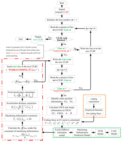
Figure 1.
Offline Feed-rate Scheduling Method for the Thin-wall Finishing Process.
2. Local Stiffness Estimation Model of Thin-Walled Parts
According to the degree of difficulty of the deformation at each position in the machining of the blade, a reasonable distribution of the feed rate can effectively solve the aforementioned problem of low overall machining efficiency of the blade. However, for machining deformation analysis, it is necessary to calculate the machining deformation of the tool-cutting position and the acceptable cutting force. Moreover, when finishing the blades, the stepovers on the machining path are usually very small, and the cutter location points are very dense. If commercial finite element software is used directly for the above simulation analysis, it will be a very large and time-consuming project. In addition, methods that rely solely on the FEM software for analysis are not sufficiently flexible. The machining deformation analysis process must be repeated when the machining parameters or cutting tools are changed.
To optimize the feed rate on the machining path, the deformation of each cutter location point under an actual cutting force was studied. These cutter location points often do not coincide with the node positions in the simulation model. To improve the analysis efficiency of the machining deformation of parts, a fast estimation method for the local stiffness of cutter location points based on the machining deformation prediction model was proposed. This is based on a previous study [31]. As shown in Figure 2, in a previous study, we combined the NURBS reconstruction method with finite element simulation results to establish a machining deformation prediction model.
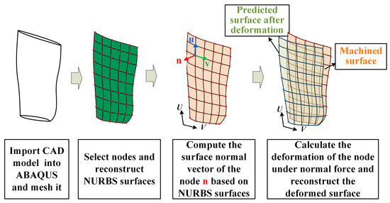
Figure 2.
Flowchart of the FEM-based machining deformation prediction model.
Based on the aforementioned machining deformation prediction model, it is considered that within the elastic range of the part, the local stiffness of a specific position on the part is relatively fixed. The local stiffness can be calculated according to Equation (1), Hooke’s law, and the analysis results of the simulation software.
where F is the normal force of the same magnitude applied to each node in the simulation software, and Ri and δi are the local stiffness and deformation of the ith node position, respectively.
Ri = F/δi
As shown in Figure 3b,c, for a smooth and continuously machined region, the variation in its local stiffness is usually continuous as well. Therefore, only the coordinates of the cutter location point and surface normal vector ni at this location need to be known. We can then determine the deformation δi of this point under any normal force, as shown in Figure 3d.
where Pd(i) is the intersection point of the line passing through point P0(i) parallel to ni and the reconstructed machining deformation prediction surface. After calculating the deformation at this point, the local stiffness can be rapidly calculated using Equation (1). Subsequently, the actual machining deformation at that point can be predicted by combining the cutting force at the cutting position. This process can be repeated to quickly calculate the local stiffness at any cutting position and predict the machining deformation for any machining parameter.
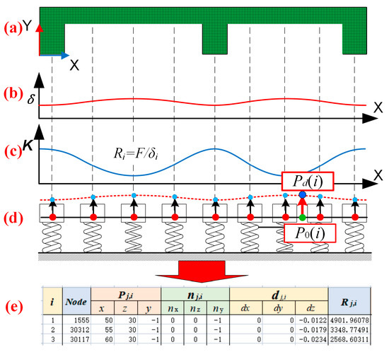
Figure 3.
Principle of establishing the local stiffness estimation model. (a) FEM model cross-section of thin-walled parts. (b) The force-induced deformation curve of the section. (c) Local stiffness curve of section. (d) Discrete spring particle model. (e) Machining deformation prediction model repre-sented by table.
The machining deformation prediction model shown in Figure 3d is fully represented by the table shown in Figure 3e. The following parameters must be included in the table: node ID, node coordinate value (x, y, z), the surface normal vector of node position (nx, ny, nz), and the deformation of each node under the same normal force (dx, dy, dz) obtained by FEM analysis. The final machining deformation prediction model was obtained using a deformed node array to reconstruct the NURBS surface. The above node information can be automatically calculated using the secondary development of the commercial finite element software ABAQUS in Python.
3. Cutting-Force Prediction Model Considering the Effect of Cutting Angle
To accurately predict machining deformation, it is necessary to precisely estimate the cutting force. Extensive research has been conducted to predict the cutting force [20,21,23,32]. Among them, the cutting-force estimation method based on experience is the most direct and convenient [32]. In this study, this empirical method was used to estimate the cutting force.
Five-axis machine tools are typically used for machining parts with special curved surfaces, such as blades. Compared with a three-axis machine tool, a five-axis machine tool has two more rotating axes; therefore, the machining process is more complicated. A typical five-axis machine tool is shown in Figure 4a. It contains two rotation coordinates: one acting on the tool and the other acting on the workpiece.
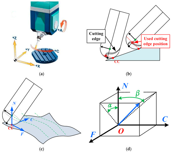
Figure 4.
Five-axis machine tool and milling cutter angle information. (a) A common five-axis machine tool. (b) Cutting edge of ball-end milling cutter. (c) The CSCS on the surface of parts in ma chining. (d) The angle parameter of the milling cutter axis expressed in the CSCS.
When machined with a five-axis machine tool, the angle between the cutter axis and the surface on which the part is machined may vary. As shown in Figure 4b, for ball-end milling cutters, the contact position between the cutter and workpiece varies with the cutter deflection angle. It should be noted that as the cutter contact (CC) point changes, the shape of the cutting edge at the contact position also changes. This situation will lead to a change in the cutting force even if the cutting parameters are the same, but with a deviation in the angle between the axis of the milling cutter and the machining surface.
An empirical model of the cutting force, including angle information of the milling process, was established. The milling force during the blade-machining process was estimated more accurately. However, neither the workpiece coordinate system nor the tool coordinate system can conveniently show the angular relationship between the tool and the machined surface. Therefore, we established a cutting surface coordinate system (CSCS) for the machining process, as shown in Figure 4c, where the origin of the CSCS coordinates corresponds to the point CC. The three axes of CSCS are the - axis along the feed direction of the tool, the N-axis along the outer normal of the surface, and the C-axis perpendicular to both the F- and N-axes.
In the establishment of the empirical model of cutting force, we chose the two angles that can reflect the spatial position of the tool in the CSCS as the parameters of the empirical model of cutting force. As shown in Figure 4d, these are the front inclination α and side inclination β. The front inclination α is the included angle between the projection of the cutter axis vector on the FON plane and the N-axis in the CSCS; the side inclination β is the angle between the projection of the cutter axis vector in the CON plane and the N-axis in the CSCS. The empirical formula for the cutting force, including the angle information of the milling process, can be expressed as
where ap is the cutting depth (mm), ae is the cutting width (mm), fZ is the feed per tooth (mm/z), vC is the cutting speed (m/min), and α and β are front inclinations and side angles, respectively. b1, b2, b3, b4, b5, and b6 are the exponential coefficients of each parameter in the above empirical formula, and CF is the coefficient of the empirical formula. The coefficients were determined using orthogonal experiments.
4. Feed-Rate Scheduling Method for Thin-Walled Blade Finishing
4.1. Identification of the Machining Process Based on the CLSF
In our method, the feed-rate scheduling process is accomplished by identifying and modifying the cutter location source file (CLSF). As shown in Figure 5, the CLSF contains information such as cutter location coordinates (CL), tool axis direction (TA), feed velocity parameter (Vf), and machining track labels.
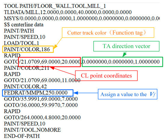
Figure 5.
Parameter information in the CLSF file.
4.1.1. Determining CC Points and the CSCS
The positions of points CC and CL during machining using a ball-end milling cutter are shown in Figure 6. As can be seen from the figure, at the contact position between the same cutter and the workpiece (CC2 point in the figure), the CL point of the milling cutter changes as the angle between the cutter and the workpiece changes. Therefore, the CL points in the CLSF cannot be directly used to represent the morphology of an actual machined surface. However, the path of the ball center (BC) of the milling cutter is an isometric line or an isometric surface on the machined surface. Therefore, we can use the BC point to estimate and represent the surface topography. Point BC can also be used to compute the normal vector on the surface of a model. The coordinates of point BC can be conveniently calculated from the information in the CLSF.
where R is the radius of the ball-end milling cutter; TA is the tool axis vector; and PCL is the CL point coordinate.
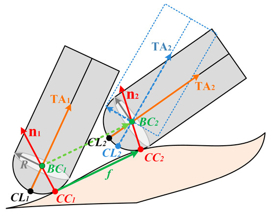
Figure 6.
CC point and CL point in the actual cutting process.
After calculating the coordinates of point BC using Equation (5), we can identify the CSCS using the point BC, as shown in Figure 7. We used the method described in the literature [33] to calculate the surface normal vector n at the position of the point BC. The coordinates of adjacent BC points were calculated by the CLSF, and their connection lines were used to determine the direction vector f (F-axis) of the feed velocity. Another direction vector on the machined surface was determined by the connection line between the current BC point and the nearest BC point in the cutting width direction. We can take the cross product of these two vectors and find the normal vector n (N-axis) at point BC. The C-axis is perpendicular to both the F-and N-axes and is easy to obtain. Thus, we determined the three axes of the CSCS. According to the definition of the CSCS in Section 3, the origin of the CSCS is the CC point. This can be obtained by normally moving point BC along the surface at a distance of one radius. The calculation process is shown in Equation (5).
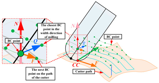
Figure 7.
Identifying the CSCS using the BC point.
4.1.2. Determining the Angle between the TA and the Machined Surface in the CSCS
After the CSCS and the tool axis vector TA are determined, the angles α and β of the tool axis in the CSCS can be calculated directly. Consider the calculation of α as an example:
First, the projection of the tool-axis vector TA onto the FON plane was calculated.
where C, N, F denote the direction vectors of the three coordinate axes of the CSCS. is the projection of TA onto the C-axis.
Then, by definition, α is the angle between and the N-axis in the CSCS, which can be calculated by the following formula:
Similarly, β can be calculated.
4.1.3. Local Stiffness Estimation and Machining Deformation Prediction at the CC Point
For parts with drastic changes in local curvature such as blades, the blades were divided into two parts: a gentle region in the middle and a region with a large curvature on both sides, as illustrated in Figure 8.
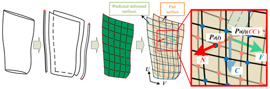
Figure 8.
Local stiffness estimation for blades.
For the gentle area in the middle of the blade, the machining deformation is mainly caused by the cutting force along the normal direction of the surface. In this region, the aforementioned method can be conveniently applied to estimate the local stiffness. However, for the edges on both sides of the blade, the force deformation is more complex. The deformation prediction model based on the normal force analysis mentioned above is not applicable to the marginal regions. Therefore, we simulated and modeled only the gentle middle region. We analyzed the large-curvature edge regions on both sides. When optimizing the feed rate in this region, it was directly reduced based on the feed rate of the previous cutter site.
4.2. Feed-Rate Optimization Constraint
The machining process must be as smooth as possible to meet the machining accuracy requirements for high-efficiency machining. We propose the following optimization and constraints:
4.2.1. Constraints on Machining Deformation Based on Local Stiffness Estimation
Ensuring machining accuracy is the primary premise of feed-rate optimization for thin-walled parts’ machining. The deformation at any position on the blade during machining should be less than the tolerance requirements of the parts. According to Equation (1), the constraint on the predicted deformation of the ith CL point can be expressed as
where Ri is the local stiffness at the point CC corresponding to the ith CL point. F[αi, βi, fZ] is the milling force at the position of the ith CL point determined by the empirical formula of cutting force. αi and βi are the front and side dip angles, respectively, of the cutter shaft at the position of the ith CL point in the CSCS. αi and βi will change depending on the cutting position and the calculation method described in the previous section. eTOL is the tolerance constraint of the blade.
After αi and βi are calculated according to the method in Section 4.1.2, cutting force can be regarded as an exponential function of feed fZ per tooth according to the empirical formula of cutting force:
where coefficient Cf is the product of the determined parameters and can be regarded as a scalar unit.
According to Equation (8), the feed velocity constraint based on local stiffness can be further described as
where ɛ is a small value, which we choose to be ɛ ≤ 0.001.
As shown in Figure 9, the maximum allowable feed per tooth (fZ)max can be quickly determined using the dichotomy method.
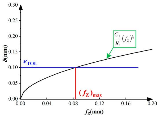
Figure 9.
Maximum feed per tooth based on local stiffness constraints.
Thus, the upper limit of the corresponding feed speed can be determined by
where D is the tool diameter (mm).
Ω is rotational speed:
vC is cutting speed (linear speed):
4.2.2. Acceleration Distance Constraint
In addition, the change in the efficiency of the feed velocity is limited by the acceleration of the machine tool. During optimization of acceleration and deceleration, we should ensure a sufficient distance between the CL points.
For two adjacent CL points, where the feed rate changes, we assume that the previous point is Pp and the current point is Pc, as shown in Figure 10. Their feed rates are (Vf)p and (Vf)c, respectively. The process from point Pp to point Pc can be divided into two stages: an accelerated feed stage (tp→tac) and a uniform feed stage (tac→tc).
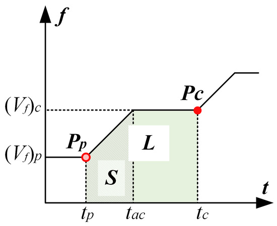
Figure 10.
Acceleration distance constraint.
In Figure 10, the polygon volume represents the distance traveled by the tool. We assume that the distance of the tool motion from Pp to Pc is L, where the distance required to complete the acceleration is S. The acceleration distance constraint can be expressed as S ≤ L.
The travel of the acceleration stage can be expressed as
where am denotes the feed acceleration of the machine tool. The feed acceleration of a typical machine tool is generally 0.5 g. The latest advanced machine tools can weigh 2 g. Here, g is the acceleration due to gravity, i.e., 1 g = 9.8 m/s2.
Given the feed velocity (Vf)p at the previous point and distance L from the current point to the previous point, the feed-speed constraint of the current point can be derived from Equation (12):
It should be noted that the units of (Vf)p and am are not uniform, and unit conversion is required in the calculation process.
4.2.3. Feed-Speed Range Constraint
Excessive feed speed leads to a reduction in the surface quality of the parts. To ensure surface quality after machining, the feed speed must be constrained according to experience.
4.3. The Execution Process of Feed-Rate Scheduling
In the previous section, we proposed three feed-rate optimization constraints for machining thin-walled blades. In the application process, they are connected in series, and the three conditions must be met simultaneously. When conducting feed-rate scheduling, we can judge the constraint range item-by-item and gradually reduce the value range of Vf. Finally, the maximum feed speed was selected to be within the optional range. Two common situations in the feed-speed scheduling process are shown in Figure 11. The final feed speed at the current point is the maximum value of the intersection region of the three constraint ranges.
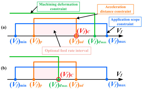
Figure 11.
Feed-rate scheduling based on constraints. (a) feed rate constrained by the acceleration distance (b) feed rate constrained by machining deformation.
The detailed execution process of the feed-rate scheduling is shown in Figure 1. This can be simply described as follows: the maximum acceptable feed speed is selected according to the local stiffness at the CL point in the CLSF file of the part. The feed-rate modification statement “FEDRAT/MMPM, ###” was inserted into the CLSF file to realize the corresponding feed-rate optimization.
5. Simulation and Experimental Verification
In the previous section, the proposed feed-rate scheduling method based on a local stiffness estimation model was introduced in detail. We conducted two sets of finishing experiments using thin-walled blades to verify the effectiveness of this method.
5.1. Experimental Setup
The machine tool used in the experiment was a five-axis linkage horizontal machining center developed by the Aviation Industry Corporation of China, as shown in Figure 12. The primary parameters of the machine tools are listed in Table 1.
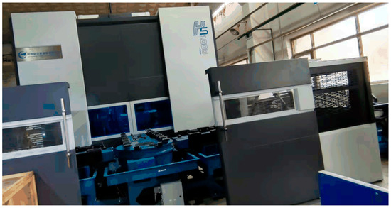
Figure 12.
Five-axis machine tool used in the experiment.

Table 1.
Machine tool parameters.
The parts used in the experiment were blades from a certain type of aeroengine. TC17 titanium–aluminum alloy was used as the material. The material parameters are listed in Table 2 [34].
Table 2.
Material parameters of the titanium–aluminum alloy TC17.
The milling cutter used in the experiment was a sintered carbide integral ball-end milling cutter with a diameter of 10 mm. The tool parameters are listed in Table 3.
Table 3.
Tool parameters.
5.2. Establishment of Milling-Force Estimation Model
Based on the cutting-force prediction model that considers the effect of the cutting angle introduced in Section 3, we designed cutting experiments to determine the values of the coefficients of each parameter in the empirical formula. Milling-force experiments were performed on the five-axis NC machining center, as described above. The milling mode involved down-milling without a coolant. A Kistler dynamometer was used to measure the milling forces during the test. The field operation of the experimental system is shown in Figure 13.
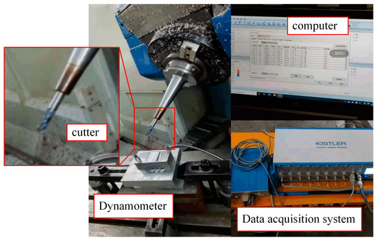
Figure 13.
Experimental device during the milling-force experiment.
The range of each parameter in the experiment was determined based on its common value range. The empirical model of the cutting force used mainly involved six process parameters. We designed an orthogonal experiment based on the orthogonal table and adopted a parameter combination of six factors and five levels. In Table 4, the left side shows the combination of the test parameters, and the right three columns show the corresponding measured results after processing. In this experiment, we considered the mean value of the measured cutting-force data as the corresponding cutting-force result.
Table 4.
Orthogonal experimental parameters and corresponding test results.
Based on the above experimental results, a multiple linear regression method was used to determine the coefficients of each parameter in the empirical formula. Finally, the empirical formula for the cutting force is
It is important to note that when applying the above empirical model of cutting forces, the actual cutting parameters used must be within the range of the process parameters used in the experiment. Only in this way can prediction accuracy be guaranteed.
5.3. Local Stiffness Estimation Model of the Blade and Its Performance Analysis
5.3.1. Local Stiffness Estimation Model of the Blade
Figure 14 shows the modeling process of the local blade stiffness estimation model based on the FEM.
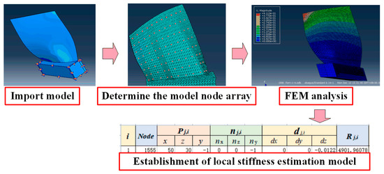
Figure 14.
Modeling process of local blade stiffness estimation based on the FEM.
First, the parts were imported into the commercial finite element software ABAQUS. The finite element model and corresponding constraints were established based on the material parameters listed in Table 2. A full constraint was established on the blade base to simulate the state of being clamped, as shown in Figure 14a. The grid was then divided. Because of the complex structure of the blade surface, a CAX4R tetrahedral mesh was used to divide the parts.
The preparatory procedure described above was completed. According to the method introduced in Section 2, evenly distributed nodes were extracted from the blade model in ABAQUS as the node array of the prediction model, as shown in Figure 14b. Subsequently, the same surface normal force was applied to each node, and a local stiffness estimation model was established using FEM analysis. As shown in Figure 14d, the local stiffness estimation model established by us based on the finite element software ABAQUS is a group of 12 × 18 node arrays.
5.3.2. Analysis of Prediction Accuracy and Efficiency of the Model
We compared the proposed local stiffness estimation model with the traditional finite element method. As shown in Figure 15, 11 nodes near the upper edge of the blade were selected as objects to compare the computational efficiencies and accuracies of the two methods.
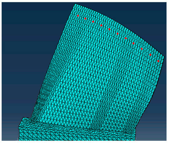
Figure 15.
The distribution of nodes on blades for comparison.
We compared the two methods on the same computer (CPU: Intel i5-1035G1 RAM:16G). The finite element software ABAQUS2016 was used for the FEM-based method. In our proposed method, VF-OPT1.2, we used automatic analysis software written by us based on Python.
During the experiment, the coordinate information of the node selected in Figure 15 and the local stiffness estimation model shown in Figure 14d were imported into the VF-OPT1.2 software. The surface normal vectors of the selected nodes and their deformation under 300 N normal force were calculated using the software. Additionally, the traditional FEM deformation prediction method was used as a control group. We directly applied a 300 N force one by one to the selected nodes in Figure 15 in ABAQUS and conducted a simulation analysis of the force-induced deformation.
Figure 16 presents a comparison of the predicted results of the two methods. The maximum prediction errors of both methods were less than 3%. This shows that the local stiffness estimation model does not sacrifice prediction accuracy. It can achieve the same precision as the prediction model based on the traditional FEM.
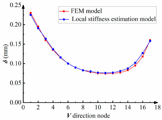
Figure 16.
Comparison of deformation prediction results between the FEM method and the proposed method.
In addition, the computational efficiencies of the two methods were compared. We also recorded the program run times for both methods. The deformation analysis process based on FEM takes approximately 274 s. However, the proposed local stiffness estimation model required approximately 0.2 s. Thus, the computational efficiency of the traditional FEM is significantly lower than that of the proposed method.
Moreover, when the machining parameters are changed, the actual cutting force changes accordingly. Using the traditional FEM-based method, the simulation analysis must be repeated to predict the amount of deformation, which is a repetitive and time-consuming process. However, the method based on the local stiffness estimation model can obtain the predicted deformation results without repeating the simulation process. Compared to the traditional FEM-based method, the proposed method is more flexible and efficient.
5.4. Application Verification of Feed-Rate Scheduling Method
Two sets of finishing experiments were conducted using thin-walled blades. The first group was the control group, which was processed with an unoptimized constant feed rate constrained by machining deformation. The machining parameters are listed in Table 5. The second group used a machining program optimized using the proposed machining method.
Table 5.
Unoptimized blade-finishing parameters.
Figure 17 shows the feed-rate distributions of the two machining programs used in the experiment, where the abscissa denotes the number of CL points, and the ordinate represents the feed rate at CL. It can be seen from the figure that the feed rate in the optimized machining program is adjusted accordingly with the change in the local stiffness of the blade. In non-optimized machining programs, the feed rate is constant.
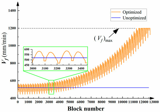
Figure 17.
Feed rate in machining before and after optimization.
Table 6 records the machining time of the blades using the above two machining methods. Compared with the unoptimized machining method, the machining efficiency of the proposed method is increased by 23%.
Table 6.
Time consumed to complete machining.
The proposed feed-rate optimization method improves the machining efficiency as much as possible while ensuring machining accuracy. The surface precision of the blade after machining is also an experimental index to be considered. Therefore, the machining errors of the two machined parts were measured and compared. After the TC17 engine blade is finished being milled, there is polishing process. Blades rely on a polishing process to improve their surface integrity [35]. While surface integrity [36] is also a key parameter to evaluate the machining effect of parts, it is not the focus of this paper.
As shown in Figure 18, two groups of nodes in the U- and V-directions of the blade were selected to measure the actual surface after machining. The measurement results are presented in Figure 19 and Figure 20. The abscissa indicates the number of measurement points, and the ordinate indicates the actual measurement error. In the U-direction, the machining error of the non-optimized program decreases gradually from top to bottom, and the margin of error reduction is large. The maximum error, which was 0.1 mm, occurred at the upper edge of the blade.
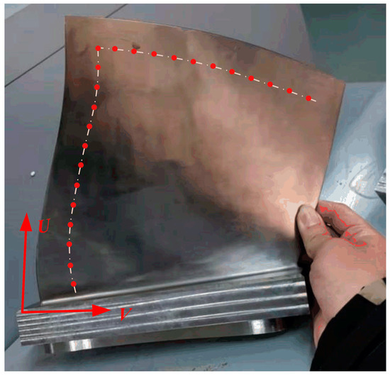
Figure 18.
The measurement scheme of the blade after being machined.
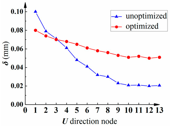
Figure 19.
Measurement results of blade in the U-direction.
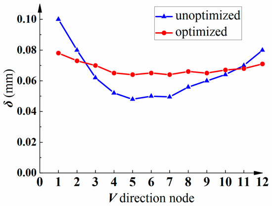
Figure 20.
Measurement results of blade in the V-direction.
The variation trend in the machining errors of the optimized program was similar to that of the non-optimized method. Moreover, the maximum machining error values were similar. However, the range of the machining errors was smaller. In the V-direction, the machining error of the non-optimized program first decreased and then increased from left to right. The maximum error appeared at the leftmost edge and was 0.1 mm. The processing error distribution of the optimized processing program was more uniform, and it was kept at approximately 0.08 mm.
The difference in the above error distribution may be caused by the fact that the machining error varies with the local stiffness of the machining position when performed using an unoptimized machining program. To ensure machining accuracy in the weak-stiffness region of the blade edge, the selected constant parameter is conservative. The machining deformation error caused by the conservative machining parameters is significantly reduced in the blade root area with high local stiffness, which is the result of sacrificing part of the machining efficiency. The optimized machining program optimizes the feed rate according to the local stiffness of the parts and determines the balance between machining accuracy and efficiency. This can improve machining efficiency while ensuring machining accuracy.
6. Conclusions
In the finishing stage of a thin-walled blade manufacture, the machining deformation factor becomes the primary problem that restricts the machining efficiency. Owing to the limitation of the machining deformation error, the parameters selected by the machining method with constant machining parameters are too conservative, and the machining efficiency is low. Offline feed-rate scheduling methods can improve the machining efficiency. However, the existing feed-rate scheduling method seldom considers the influence of machining deformation factors; therefore, it cannot be applied to feed-rate optimization in the finishing stage of thin-walled blades.
To solve these problems, an offline feed-rate scheduling method for blade finishing based on a local stiffness estimation model was proposed. In this method, a fast estimation model for the local stiffness of thin-walled blades and an empirical model for cutting-force estimation, including cutting angle information, was established. Based on the above model, a feed-rate optimization method that considers the machining deformation and surface smoothness constraints is proposed. Finally, the optimization of the proposed method is verified by performing actual finishing experiments on two thin-walled blades. The test results were as follows:
- A machining method with constant cutting parameters is constrained by the machining deformation error during the machining of thin-walled blades, resulting in conservative machining parameters and low machining efficiency.
- Compared with the FEM-based model, the maximum prediction error of the established local stiffness estimation model is less than 3%, but the calculation time is reduced by 99%. This shows that the proposed local stiffness estimation model has a higher computational efficiency and flexibility.
- The proposed offline feed-rate scheduling method increases the machining efficiency by 23% and reduces the machining error by 20%. This shows that the proposed method can reasonably allocate the feed rate and improve the machining efficiency of parts while ensuring the machining accuracy of thin-walled blades.
In addition, the proposed method is universal. It can be conveniently applied to other thin-walled parts with large continuous machined surfaces.
Author Contributions
Conceptualization, L.W., A.W., and W.X.; validation, W.X.; formal analysis, L.W.; investigation, L.W., A.W., and W.X.; writing—review and editing, L.W.; supervision, A.W. All authors have read and agreed to the published version of the manuscript.
Funding
The authors would like to express their thanks for the gracious financial support from the National Key Research and Development Project of China (No. 2020YFB1713100).
Data Availability Statement
Data are contained within the article.
Conflicts of Interest
The authors declare no conflict of interest.
References
- Kurt, M.; Bagci, E. Feedrate optimisation/scheduling on sculptured surface machining: A comprehensive review, applications and future directions. Int. J. Adv. Manuf. Technol. 2011, 55, 1037–1067. [Google Scholar] [CrossRef]
- Adams, O.; Klocke, F.; Schwenzer, M.; Stemmler, S.; Abel, D. Model-based predictive force control in milling—System identification. Procedia Technol. 2016, 26, 214–220. [Google Scholar] [CrossRef]
- Han, Z.; Jin, H.; Fu, Y.; Fu, H. Cutting deflection control of the blade based on real-time feedrate scheduling in open modular architecture CNC system. Int. J. Adv. Manuf. Technol. 2017, 90, 2567–2579. [Google Scholar] [CrossRef]
- Jang, D.; Kim, K.; Jung, J. Voxel-based virtual multi-axis machining. Int. J. Adv. Manuf. Technol. 2000, 16, 709–713. [Google Scholar] [CrossRef]
- Layegh, K.S.E.; Erdim, H.; Lazoglu, I. Offline force control and feedrate scheduling for complex free form surfaces in 5-axis milling. Procedia CIRP 2012, 1, 96–101. [Google Scholar]
- Woo, W.-S.; Curtis, D.; Bagni, C.; Lee, C.-M.; Lee, J.-H.; Kim, D.-H. Productivity enhancement of aircraft turbine disk using a two-step strategy based on tool-path planning and NC-code optimization. Metals 2022, 12, 567. [Google Scholar] [CrossRef]
- Käsemodel, R.B.; de Souza, A.F.; Voigt, R.; Basso, I.; Rodrigues, A.R. CAD/CAM interfaced algorithm reduces cutting force, roughness, and machining time in free-form milling. Int. J. Adv. Manuf. Technol. 2020, 107, 1883–1900. [Google Scholar] [CrossRef]
- Ghosh, T.; Wang, Y.; Martinsen, K.; Wang, K. A surrogate-assisted optimization approach for multi-response end milling of aluminum alloy AA3105. Int. J. Adv. Manuf. Technol. 2020, 111, 2419–2439. [Google Scholar] [CrossRef]
- Park, H.; Qi, B.; Dang, D.; Park, D.Y. Development of smart machining system for optimizing feedrates to minimize machining time. J. Comp. Des. Eng. 2018, 5, 299–304. [Google Scholar] [CrossRef]
- Wang, L.P.; Yuan, X.; Si, H.; Duan, F.Y. Feedrate scheduling method for constant peak cutting force in five-axis flank milling process. Chin. J. Aeronaut. 2020, 33, 2055–2069. [Google Scholar] [CrossRef]
- Zhang, Z.; Luo, M.; Zhang, D.; Wu, B. A force-measuring-based approach for feed rate optimization considering the stochasticity of machining allowance. Int. J. Adv. Manuf. Technol. 2018, 97, 2545–2556. [Google Scholar] [CrossRef]
- Osorio-Pinzon, J.C.; Abolghasem, S.; Marañon, A.; Casas-Rodriguez, J.P. Cutting parameter optimization of Al-6063-O using numerical simulations and particle swarm optimization. Int. J. Adv. Manuf. Technol. 2020, 111, 2507–2532. [Google Scholar] [CrossRef]
- Xu, G.; Chen, J.; Zhou, H.; Yang, J.; Hu, P.; Dai, W. Multi-objective feedrate optimization method of end milling using the internal data of the CNC system. Int. J. Adv. Manuf. Technol. 2019, 101, 715–731. [Google Scholar] [CrossRef]
- Xie, J.; Zhao, P.; Hu, P.; Yin, Y.; Zhou, H.; Chen, J.; Yang, J. Multi-objective feed rate optimization of three-axis rough milling based on artificial neural network. Int. J. Adv. Manuf. Technol. 2021, 114, 1323–1339. [Google Scholar] [CrossRef]
- Wu, B.; Zhang, Y.; Liu, G.; Zhang, Y. Feedrate optimization method based on machining allowance optimization and constant power constraint. Int. J. Adv. Manuf. Technol. 2021, 115, 3345–3360. [Google Scholar] [CrossRef]
- Du, X.; Huang, J.; Zhu, L.-M.; Ding, H. An error-bounded B-spline curve approximation scheme using dominant points for CNC interpolation of micro-line toolpath. Robot. Comput. Integr. Manuf. 2020, 64, 101930. [Google Scholar] [CrossRef]
- Li, H.; Jiang, X.; Huo, G.; Su, C.; Wang, B.; Hu, Y.; Zheng, Z. A novel feedrate scheduling method based on Sigmoid function with chord error and kinematic constraints. Int. J. Adv. Manuf. Technol. 2022, 119, 1531–1552. [Google Scholar] [CrossRef]
- Song, D.N.; Ma, J.W.; Zhong, Y.G.; Xiao, D.; Yao, J.J.; Zhou, C. A fully real-time spline interpolation algorithm with axial jerk constraint based on FIR filtering. Int. J. Adv. Manuf. Technol. 2021, 113, 1873–1886. [Google Scholar] [CrossRef]
- Zhang, Y.; Ye, P.; Zhao, M.; Zhang, H. Dynamic feedrate optimization for parametric toolpath with data-based tracking error prediction. Mech. Syst. Signal Process. 2019, 120, 221–233. [Google Scholar] [CrossRef]
- Lamikiz, A.; López de Lacalle, L.N.; Sánchez, J.A.; Salgado, M.A. Cutting force estimation in sculptured surface milling. Int. J. Mach. Tools Manuf. 2004, 44, 1511–1526. [Google Scholar] [CrossRef]
- Calleja, A.; Alonso, M.A.; Fernández, A.; Tabernero, I.; Ayesta, I.; Lamikiz, A.; López de Lacalle, L.N. Flank milling model for tool path programming of turbine blisks and compressors. Int. J. Prod. Res. 2014, 53, 3354–3369. [Google Scholar] [CrossRef]
- Calleja, A.; Bo, P.; González, H.; Bartoň, M.; López de Lacalle, L.N. Highly accurate 5-axis flank CNC machining with conical tools. Int. J. Adv. Manuf. Technol. 2018, 97, 1605–1615. [Google Scholar] [CrossRef]
- Salgado, M.A.; López de Lacalle, L.N.; Lamikiz, A.; Muñoa, J.; Sánchez, J.A. Evaluation of the stiffness chain on the deflection of end-mills under cutting forces. Int. J. Mach. Tools Manuf. 2005, 45, 727–739. [Google Scholar] [CrossRef]
- López de Lacalle, L.N.; Lamikiz, A.; Sánchez, J.A.; Salgado, M.A. Toolpath selection based on the minimum deflection cutting forces in the programming of complex surfaces milling. Int. J. Mach. Tools Manuf. 2007, 47, 388–400. [Google Scholar] [CrossRef]
- Hou, Y.; Zhang, D.; Zhang, Y.; Wu, B. The variable radial depth of cut in finishing machining of thin-walled blade based on the stable-state deformation field. Int. J. Adv. Manuf. Technol. 2021, 113, 141–158. [Google Scholar] [CrossRef]
- Wang, J.; Ibaraki, S.; Matsubara, A. A cutting sequence optimization algorithm to reduce the workpiece deformation in thin-wall machining. Precis. Eng. 2017, 50, 506–514. [Google Scholar] [CrossRef]
- Campa, F.J.; Lopez de Lacalle, L.N.; Celaya, A. Chatter avoidance in the milling of thin floors with bull-nose end mills: Model and stability diagrams. Int. J. Mach. Tools Manuf. 2011, 51, 43–53. [Google Scholar] [CrossRef]
- Rozylo, P.; Debski, H. Effect of eccentric loading on the stability and load-carrying capacity of thin-walled composite profiles with top-hat section. Compos. Struct. 2020, 245, 112388. [Google Scholar] [CrossRef]
- Wysmulski, P.; Debski, H.; Falkowicz, K.; Rozylo, P. The influence of load eccentricity on the behavior of thin-walled compressed composite structures. Compos. Struct. 2019, 213, 98–107. [Google Scholar] [CrossRef]
- Hailong, M.; Aijun, T.; Shubo, X.; Tong, L. Finite element simulation of bending thin-walled parts and optimization of cutting parameters. Metals 2023, 13, 115. [Google Scholar] [CrossRef]
- Wu, L.; Wang, A.; Xing, W.; Wang, K. Adaptive sampling method for thin-walled parts based on on-machine measurement. Int. J. Adv. Manuf. Technol. 2022, 122, 2577–2592. [Google Scholar] [CrossRef]
- Fei, J.; Xu, F.; Lin, B.; Huang, T. State of the art in milling process of the flexible workpiece. Int. J. Adv. Manuf. Technol. 2020, 109, 1695–1725. [Google Scholar] [CrossRef]
- Tunc, L.T. Rapid extraction of machined surface data through inverse geometrical solution of tool path information. Int. J. Adv. Manuf. Technol. 2016, 87, 353–362. [Google Scholar] [CrossRef]
- Gerhard, W.; Boyer, R.R.; Collings, E.W. Material Properties Handbook: Titanium Alloys; ASM International: Materials Park, OH, USA, 1994. [Google Scholar]
- Liu, D.; Shi, Y.; Lin, X.; Xian, C.; Gu, Z. Polishing surface integrity of TC17 aeroengine blades. J. Mech. Sci. Technol. 2020, 34, 689–699. [Google Scholar] [CrossRef]
- Fernandez-Valdivielso, A.; de Lacalle, L.N.L.; Urbikain, G.; Rodriguez, A. Detecting the key geometrical features and grades of carbide inserts for the turning of nickel-based alloys concerning surface integrity. Proc. Inst. Mech. Eng. Part C J. Mech. Eng. Sci. 2016, 230, 3725–3742. [Google Scholar] [CrossRef]


Disclaimer/Publisher’s Note: The statements, opinions and data contained in all publications are solely those of the individual author(s) and contributor(s) and not of MDPI and/or the editor(s). MDPI and/or the editor(s) disclaim responsibility for any injury to people or property resulting from any ideas, methods, instructions or products referred to in the content. |
© 2023 by the authors. Licensee MDPI, Basel, Switzerland. This article is an open access article distributed under the terms and conditions of the Creative Commons Attribution (CC BY) license (https://creativecommons.org/licenses/by/4.0/).