Abstract
The vibrational behavior of components in mechanical systems like drives and robots can become critical under changes in the system properties or loading in operation. Such undesired vibration can lead to detrimental conditions including excess wear, fatigue, discomfort, and acoustic emissions. Systems are designed to avoid certain frequencies to avoid such problems, but system parameters can change during operation due damage, wear, or change in loading. An example is the change in system properties or operation state that then activates resonance frequencies in our system. Therefore, this work has the goal of modifying the modal behavior of a system to avoid vibrational problems. Methods of design optimization are applied to find a new optimum design for this altered condition. Here, this is limited to the addition of mass in order to move the resonance frequency out of critical ranges. This though requires a new formulation of the optimization problem. We propose a new constraint formulation to avoid frequency ranges. To increase efficiency, a reduced analytical sensitivity analysis is introduced. This methodology is demonstrated on two test cases: a two-mass oscillator followed by a test case of higher complexity which is a gear housing considering over 15,000 design variables. The results show that the optimization solution gives the position and amount of mass added, which is a discrete solution that is practically implementable.
1. Introduction
In this study, a design methodology is introduced to redesign mechanical systems to account for changes in system parameters or other environmental changes during operation. To limit the encroachment on an in-operation mechanical system, the changes of the system are confined to the addition of mass to the exterior of a housing. Hereby, we desire to find the optimal position and amount of added mass so that the vibrational behavior will be changed and eigenfrequencies pushed out of critical frequency bands. After the derivation of the methodology, it will be shown on two cases of increasing complexity: first on a two-mass oscillator and then on the housing of a planetary gear set assembly.
The developed methodology is applicable in cases in which damage and wear alter the vibrational behavior and specifically the eigenfrequencies. An example of changes in system parameters is a changed mesh stiffness of a planetary gear set that causes the vibrational excitation of the housing. The excitation of the housing is considered unacceptable as this will cause increased wear of components connected to the housing and acoustic emissions.
Here, we use numerical optimization to find the minimum added mass to move the eigenfrequencies out of certain frequency bands. It should be noted that it is intrinsic that added mass leads only to a reduction in the values of eigenfrequencies. The optimally in-operational redesigned eigenfrequencies will be lower, but importantly out of critical frequency bands to avoid excitation. This type of solution is a pragmatic temporary fix until the machine can be shutdown and maintenance performed to ensure the original design performance.
Optimal design of mechanical systems under dynamic considerations stems from two traditions and seemly separate communities denoted by the terms: structural design optimization (also structural optimization or design optimization, see Ross [1], Baier et al. [2], Vanderplaats [3]) and dynamic structural modification (also structural dynamic modification or simply structural modification, see Bucher and Braun [4], He [5], Avitabile [6], Belotti and Richiedei [7]).
The latter includes the assignment of the eigenpair (eigenfrequency or mode shape or both) via an inverse problem formulation. This method is typically shown on lumped-parameter models and beam models of few degrees of freedom. Structural design optimization on the other hand varies from small beam problems to large finite-element models with several million degrees of freedom. Formulations include dynamics often as constraints and mass as the objective, especially in the framework of lightweight design. Both of these families of methodologies are algorithmic-supported design mechanical systems or structures. The governing equation of both is the eigenvalue problem resulting in eigenvalues (eigenfrequencies or resonance frequencies) and eigenvectors (mode shapes). The transient response and frequency response functions are also of interest in certain cases but are not considered here.
This work aims to reduce vibration by adding a minimum amount of mass in a similar optimization formulation as introduced by Pritchard et al. [8]. The constraint formulation is based on the formulation introduced by Ross [1] and further developed in its parabolic form in Wehrle et al. [9]. The ballistic frequency-range constraint was developed in this study. A large number of design variables is feasible with gradient-based optimization with analytical sensitivity analysis [10,11,12,13]. Specifically, the sensitivities of eigenfrequencies, also known as eigensensitivities, are carried out in an efficient reduced form introduced here, allowing for a sensitivity analysis that has a computational effort that is a fraction of that of the original eigenvalue problem.
Examples will be shown with both a lumped-parameter model as well as a finite-element model. The latter shows the methodology with a large-scale problem, both in terms of the number of design variables and of the number of degrees of freedom.
2. Design Optimization for In-Operation Structural Modification
In this work, we find the optimal position and amount of mass added to change the vibrational behavior—specifically the eigenfrequencies—of a system. Added mass can, for example, be easily added to the exterior of a housing with a limited intervention to the system, which is typically possible during in-operational conditions, requiring only a short stoppage if at all. To accomplish this, and specifically to properly design the position and amount of mass added, this engineering design problem is expressed as a numerical optimization problem. The formulation of the constraints concerning frequency bands are of special interest. To ensure a computational effort of reasonable magnitude, an efficient sensitivity analysis is developed here and derived below.
2.1. Formulation and Setup of the Optimization Problem
In contrast to the classic dynamic structural modification problem in which specific eigenfrequencies and mode shapes are desired, we wish to avoid frequency bands by adding a minimum amount of mass. Therefore, an inverse problem formulation is not possible and instead we will use a formulation using structural design optimization that are solved with a numerical optimization algorithm. Structural design optimization is formulated generally as
where f is the objective function, g a constraint function, y a constrained system response, c the state limit, the vector of design variables within a design domain χ, which is defined by the vectors of the lower bounds and the upper bounds . Here, the constraint functions are formulated in the form of upper bound constraints. It should be noted that we denote here matrices as double underlined symbols , vectors are underlined , and scalars have no underline. This applies to both upper and lower cases symbols.
In this study, the design variables are the added masses at discrete points and the constraint functions will be the natural frequencies, which are constrained in certain ranges. We will be minimizing the sum of added masses to
- 1.
- minimize the change in our structural behavior, which could possibly lead to other problems,
- 2.
- avoid added mass that can often lead to lowered efficiency.
2.2. Frequency-Band Constraints
In this study, the goal is to avoid resonance problems. Therefore, several ranges of eigenfrequencies of a dynamic system are to be constrained, which we refer to as frequency-band constraints (see Figure 1). In the following, constraint formulations that avoid ranges will be introduced: first a formulation from the literature, then a derived formulation, and finally a novel formulation specifically developed here.
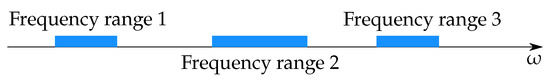
Figure 1.
Schematic of frequency-band constraints.
A frequency-band constraint formulation was introduced by [1] to constrain ranges of frequencies in which the frequency band constraints are defined by
Each constraint function g is defined by
where is the jth calculated eigenfrequency, while and are the lower and upper-bound frequencies of the kth frequency-band constraint. Inspired by the Ross formulation, we limit the polynomial as a second-order function and introduce further constraints, which takes the following form:
where is a constant to normalize the constraint values keeping the same maximum value of all and is the running index from zero to . This formulation requires constraint functions. It should be noted that the constraint convention here is that negative values are a feasible design while positive values are nonfeasible. As can be seen in Figure 2, the parabolic constraint formulation results in a parabola over each of the constrained frequency band. This formulation has also been successfully applied to planetary gear design in Wehrle et al. [9], Wehrle et al. [14], Wehrle et al. [15].
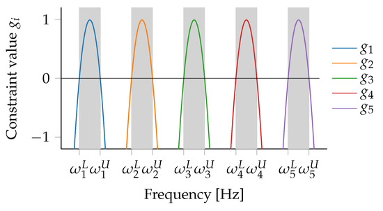
Figure 2.
An example of the parabolic formulation for frequency-band constraints where the ranges to be avoided are gray, and each colored line represents a constraint function.
As here only mass is added, which results in intrinsically lower resonance frequencies, a saw-tooth constraint function was first devised. This was done to avoid problems that may occur with a gradient-based optimization algorithm when the position of the frequency to be moved would be located on the section of the parabola with negative slope (i.e., higher than the midpoint of the frequency range). To avoid a non-differentiable piecewise representational, as is the case of the saw tooth function, a continuous approximation of the saw tooth function was found. Recognizing that the continuous function of that of the ballistic trajectory of a projectile with drag, we define this novel constraint formulation, which we will refer to as ballistic frequency-range constraint, as
which depends on the constants a, b, c, and d. It should be noted that this function is normalized to have a maximum value of unity. The constants a and b are chosen to define the shape, while c and d are dependent on the former. The value for a is chosen on the interval and defines how much the peak is moved away from the center of the range. The value for b is set to 0 or to define if the peak is moved in direction of the upper or lower limit of the range constraint. The two constants c and d are defined as follows:
where is the multivalued inverse of the Lambert W-function of , which has an infinite number of branches. Each of the branches has a different solution to
for any complex number z and any branch index k. The Lambert W-function has a real value for the principal branch on the interval and for the branch on the interval [16] (see Figure 3). Since in our case the Lambert W-function is used by and , the resulting value is real and on the interval . It should be noted that the value of the ballistic trajectory inspired constraint formulation converges to the constraint from Ross [1] for small values of a,
and, therefore, the ballistic-trajectory-inspired constraint formulation can be considered as a generalization of the parabolic formulation. Figure 4 shows the different forms that the ballistic constraint formulation can assume: left or right leaning and the sharpness of the peak. For different optimization formulation, different forms may be beneficial. In this work, a right leaning function with a sharp peak was chosen.
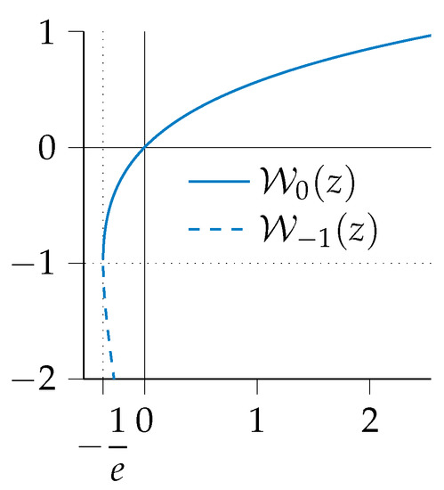
Figure 3.
The two real branches of [16].
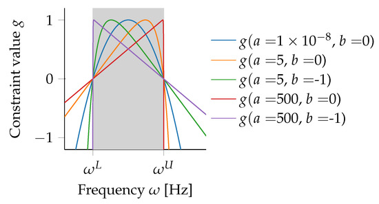
Figure 4.
Different profiles of the ballistic range constraint function.
As the value of the constraint functions can easily reach a large negative value in the feasible domain, this can have negative infinity in its computer implementation. To avoid numerical issues and errors, we use a large negative number, here . As these designs are feasible, this has no negative effect with gradient-based optimization algorithms.
It should be duly noted that this formulation results in a non-convex design domain. Figure 5 shows how this formulation has an inherently non-convex design domain for the two-mass oscillator optimized in Section 3.1.
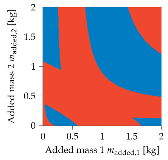
Figure 5.
Design domain of the two-mass oscillator with valid (blue) and invalid (red) design domain demonstrating islands of validity.
This being the case, the pragmatic use of gradient-based optimization algorithms is shown to efficiently solve this design problem.
2.3. Sensitivity of Added Mass
To ensure computational efficiency, gradient-based optimization is used for this redesign problem. Therefore, the analytical sensitivities are provided to reduce the computational effort. For the Hermitian eigenvalue problem (undamped case) and where the eigenvector is normalized about the mass matrix, i.e., , the eigenfrequency sensitivity is [2,17]
It should be noted that we use the nomenclature here where is the total derivative of some function with respect to the vector and is the partial derivative with respect to one term of the vector , namely . Specifically in our case, there will be no change in stiffness and therefore the eigenfrequency sensitivity simplifies to
As we are adding mass to mass points, the term is a matrix with ones on the diagonal at those corresponding degrees of freedom and elsewhere empty. This study utilizes this matrix structure and introduces a novel approach to drastically reduce the dimensionality of the sensitivity analysis and therefore the computational effort. We can reduce the size of this equation to three degrees of freedom for the spatial case, two for the planar case and one for the one-degree of freedom case, i.e., is simply the identity matrix with the size of the numbers of dimension of the model. Therefore, assuming a lumped mass matrix for a mass point, these values are the following:
The mass sensitivity matrix and mode vector reduce to those degrees of freedom of the mass point affected by a single design vector ; all other values of the mass sensitivity matrix are zero. The reduction of can be shown with the following graphical representations of the sensitivity equation:
 |
and, as is the identity matrix, this simplifies to the following:
 |
Summarizing, for the sensitivity of the jth natural frequency to the ith design variables, gives the following:
where the subscript i of refers to the degrees of freedom of the ith design variable. The sensitivity equation then reduces to a simple function proportional to the square of the eigenvector of those degrees of freedom of the node of added mass. In turn this drastically reduces the computational effort of the senstivity analysis.
2.4. Sensitivity Formulations of Frequency-Band Constraints
Above, we derived the sensitivities of the eigenfrequencies with respect to added mass. The final sensitivity of the constraint functions is needed by the optimization algorithm. The constraint formation by Ross [1] has the following sensitivity (also developed within the same work):
We now introduce the sensitivities of the range-constraint functions introduced in this work. The parabolic range-constraint function has the following sensitivity:
This work introduces the ballistic range-constraint formulation and this design sensitivity can be calculated by
The last of these is the sensitivity function that will be used in the examples below.
3. Numerical Validation
3.1. Two-Mass Oscillator
The method described above will be shown on an introductory example of the two-mass oscillator (Figure 6). We have an original design of the following parameters:
giving the following eigenfrequencies of the system
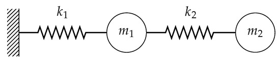
Figure 6.
Schematic of two-mass oscillator.
It is now assumed that the eigenbehavior of the system has shifted due to wear or fault, or that the requirements have changed. The constrained regions are defined by
which gives a nonfeasible initial design. A design is to be found in which these frequency ranges are avoided by adding a minimum mass to the system. The resulting design domain of this two-dimensional problem is displayed above in Figure 5. The optimization formulation is
As added mass can only lower the eigenfrequency, the ballistic constraint function is used here with constant values and , resulting in a continuous saw-tooth form, cf. Section 2.2 and Figure 4. The optimal design of a two-mass oscillator is solved using the first-order optimization algorithm, method of moving asymptotes (MMA) [18] with the above-described analytical sensitivity method. Despite the non-convex design domain as a result of the frequency-band constraints (cf. Section 2.2 and Figure 2), it has been shown in [9,14,15] that gradient-based optimization algorithms are efficient and effective. The main design goal here is achieving a feasible design and therefore the risk of the optimum being not globally optimal is acceptable.
Starting from the lower limit, i.e., the original design, this optimization problem quickly finds a valid design with minimum amount off added mass. With MMA, this needs 11 iterations, which in turn requires 11 system evaluations and 11 sensitivity evaluations. The convergence plot is seen in Figure 7. The start and optimal values are found in Table 1.
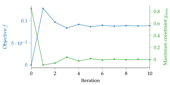
Figure 7.
Convergence plot for the two-mass oscillator.

Table 1.
Optimization responses for the two-mass oscillator.
3.2. Gear Housing
Here, we will show the application of the developed methodology to a large-scale engineering example. A housing of a planetary gear set will be redesigned to find the position and amount of added mass to move it out of critical frequency ranges.
The vibrational behavior of the gear housing is assessed via an eigenvalue analysis of a three-dimensional model with the finite-element method. The geometry is shown in Figure 8. The base of the housing is sized and its height is . The eigenvalue problem of the structural-mechanical model with neglected damping and free vibration is given by
where is the mass matrix, is the stiffness matrix, is the jth eigenfrequency (the square root of the eigenvalue), and is the corresponding jth mode shape (eigenvector). This analysis is solved using the open software Kratos Multiphysics [19,20]. The finite-element model consists of 195,970 nodes and 1,077,626 volume elements. It is made of steel and a linear elastic material model is applied with the parameters shown in Table 2. The bottom face (highlighted in orange in Figure 8b) is clamped to restrict the structure.
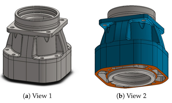
Figure 8.
Geometry of the gear housing with design domain shown in blue.
Table 2.
Linear-elastic material properties of steel.
We limit the scope of the analysis and optimal design to the first six eigenfrequencies, whose mode shapes can be seen in Figure 9.
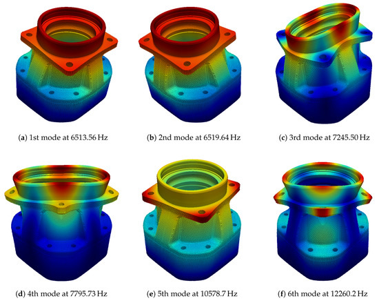
Figure 9.
First six mode shapes of the gear housing.
Studies about the modeling of vibrational behavior of planetary gear sets and the determination of the uncertain eigenfrequencies are introduced by Wehrle et al. [14], Wehrle et al. [15].
Table 3 summarizes the frequency ranges which should be avoided by the eigenfrequencies of the housing.
Table 3.
Frequency bands to be avoided.
A comparison of these frequency ranges and the computed values show that some eigenfrequencies of the housing are in the forbidden ranges. To move the eigenfrequencies outside of the forbidden frequency ranges, mass can be added to the housing. In this application, mass can be added to all mesh nodes which are on the external surface of the housing, highlighted in blue in Figure 8b.
The engineering design problem described above is implemented as a numerical optimization problem of the following form:
where the constraint index . The objective function is the minimization of the added mass. The constraint formulation and sensitivity analysis are performed as described above in Section 2.2, Section 2.3 and Section 2.4. As added mass can only lower the eigenfrequency, the ballistic range constraint function is used with the constants and , which is like the two-mass oscillator results in a continuous saw-tooth form, cf. Figure 4. Design variables are all surface nodes on the highlighted blue surface in Figure 8b. With this, the vector of design variables are the values of the mass added to these 15,494 nodal mass elements. The lower bound of the design variables is set to zero,
and the upper bound of the design variables is set to a value of
The start vector of the design variables is set to the lower bound values, i.e., the initial structure with no added mass. The design optimization is performed using the toolbox DesOptPy [21,22] and the first-order optimization algorithm MMA [18].
Figure 10 shows the values of eigenfrequency sensitivities of the initial design (i.e., with no added mass). The sensitivities are calculated by eigenfrequency and the value of the sensitivity with respect to each design variable, i.e., nodal mass, is represented by the color of the spheres shown in each subfigure. It should be noted that the flat gray (i.e., without spheres) has been designated as non-design domain. As per Equation (17), the relation between mode shape and sensitivities can be clearly seen, cf. Figure 9 and Figure 10. The solution of the eigenvalue problem for the first six modes at the initial design requires approximately nine minutes on a machine with an Intel Core i7-8700 CPU at 3.20 GHz × 12 and 31.4 GiB of random-access memory. The efficiency of the optimization technique is guaranteed with sensitivity computations, which with the method described in Section 2.3 takes less than one second.
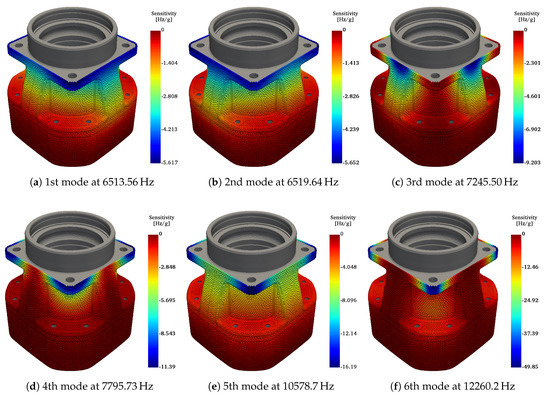
Figure 10.
Sensitivities of the eigenfrequencies of the gear housing with respect to added mass
Figure 11 shows the values of the objective function and the maximum constraint function during the optimization run. Convergence was reached after 28 iterations and a feasible design is obtained. It is here to see that the problem immediately moves to a feasible design after the second iteration and after which the added mass is further reduced while staying at the active constraint limit. This excellent convergence behavior is obtained with the gradient-based algorithm despite the non-convex nature of the problem, including islands of feasibility (cf. Figure 5). For the optimal design, of mass was added to the housing, which has a mass of , or only a 2% increase in mass with respect to its initial mass. Furthermore, as the design is feasible, all eigenfrequencies have been shifted out of the constrained ranges. The numerical results can be seen in Table 4 and Table 5.
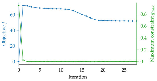
Figure 11.
Convergence plot for the housing.
Table 4.
Optimization responses for the gear housing.
Table 5.
Optimal values of the design variables for the gear housing, all values in g.
After the design optimization, the vast majority of design variable values are numerically zero, creating a favorably discrete solution. In fact, of the 15,494 design variables, there are only 17 with values larger than zero, i.e., only 17 nodal mass elements have added mass. The values of these are found in Table 5. Figure 12 shows the position of the zero design variables in gray and the design variables with different values in the scale of the color bar. Of the 17 design variables with an added mass, four optimal values are at the upper limit of , one optimal value is approximately , and a further optimal value is approximately . The optimal values of the other 11 design variables are one to three magnitudes smaller and have values between and , which are identified in Figure 12 as yellow mass nodes. The optimal positions are be nearly symmetrical at the top edge of the upper flange. That so few nodes of the optimal design have added mass is deemed to be positive and, therefore, easier to physically implement.
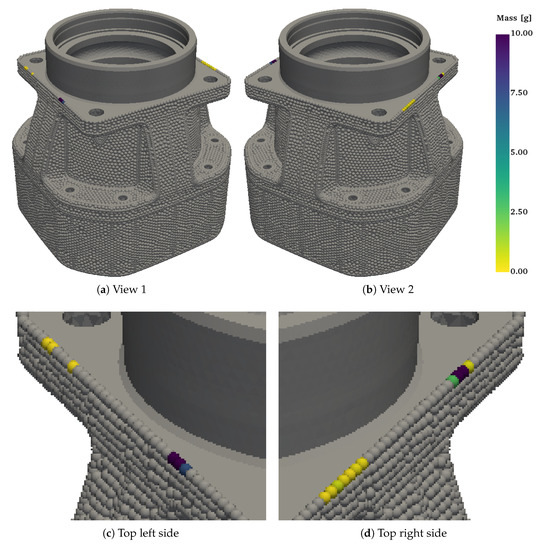
Figure 12.
Values of design variables after optimization; nodes with zero mass are shown in gray, nodes with added mass are shown with the scale of the color bar.
4. Conclusions
In this work, we have developed a new methodology for the efficient redesign of mechanical systems with respect to their eigenfrequencies by adding mass. The solution results in the amount and position of mass to be added. Due to the generality of this method, it can be applied to small lumped-parameter models or very large finite-element models efficiently and effectively. This is validated above on two case studies.
It was shown that, even with the simple test case with few design variables, the design domain is multimodal and has islands of validity. Therefore, this problem is inherently non-convex. Despite this characteristic of the optimization problem, gradient-based algorithms were used because of their great efficiency and successfully moved the eigenfrequencies of the system outside the constrained bands. Although the gradient-based algorithms lead to a final design that is a local minimum, the non-convexity of the problem cannot guarantee that this is a global minimum. With such large design domains as the engineering example, the main priorities were feasibility of design and efficiency, which were achieved.
As this method is efficient, when models are a priori available, this can be also carried out online to properly design addition mass to alter the vibrational behavior in the matter of minutes or even seconds. Furthermore, in this case, the objective function was chosen to minimum added mass, which leads to the least change in the system.
For the practical application of this methodology, only an accurate CAD model of the housing and the frequency ranges that are to be avoided are necessary. After meshing, a node set is defined on the exterior of the housing on which the addition of mass is feasible. There may be manufacturing inaccuracies and material variations causing deviations from the deterministic values used here. Uncertainty analysis can then also be integrated into the design process. Experimental studies are planned for both this investigation as well as the general verification using different benchmark examples.
For a wide range of applications, the addition of mass, e.g., to the outside of the housing, represents an ideal solution to maintain other operating conditions. In this work, it is shown that this can be done with a design optimization method utilizing a new constraint formulation and efficient sensitivity analysis. The method can further be extended to include other objectives, design variables and constraints.
Author Contributions
E.W.: Conceptualization, Investigation, Funding Acquisition, Methodology, Project Administration, Software, Supervision, Validation, Visualization, Writing—Original Draft Preparation, and Writing—Reviewing and Editing; V.G.: Investigation, Methodology, Software, Validation, Visualization, Writing—Original Draft Preparation, and Writing—Reviewing and Editing. R.V.: Supervision and Writing—Reviewing and Editing. All authors have read and agreed to the published version of the manuscript.
Funding
This work is supported by the project CRC 2017–TN2091 doloMULTI Design of Lightweight Optimized structures and systems under MULTIdisciplinary considerations through integration of MULTIbody dynamics in a MULTIphysics framework funded by the Free University of Bozen-Bolzano. This work was supported by the Open Access Publishing Fund provided by the Free University of Bozen-Bolzano.
Conflicts of Interest
The authors declare no conflict of interest.
References
- Ross, C. Strukturoptimierung mit Nebenbedingungen aus der Dynamik. Ph.D. Thesis, Technische Universität München, Munich, Germany, 1991. [Google Scholar]
- Baier, H.; Seeßelberg, C.; Specht, B. Optimierung in der Strukturmechanik; Vieweg: Braunschweig, Germany, 1994. [Google Scholar]
- Vanderplaats, G.N. Multidiscipline Design Optimization; Vanderplaats Research & Development: Colorado Springs, CO, USA, 2007. [Google Scholar]
- Bucher, I.; Braun, S. The structural modification inverse problem: An exact solution. Mech. Syst. Signal Process. 1993, 7, 217–238. [Google Scholar] [CrossRef]
- He, J. Structural modification. Philos. Trans. R. Soc. A Math. Phys. Eng. Sci. 2001, 359, 187. [Google Scholar] [CrossRef]
- Avitabile, P. Twenty years of structural dynamic modification—A review. Sound Vib. 2003, 37, 14–27. [Google Scholar]
- Belotti, R.; Richiedei, D. Designing auxiliary systems for the inverse eigenstructure assignment in vibrating systems. Arch. Appl. Mech. 2017, 87, 171–182. [Google Scholar] [CrossRef]
- Pritchard, J.I.; Adelman, H.M.; Haftka, R.T. Sensitivity analysis and optimization of nodal point placement for vibration reduction. J. Sound Vib. 1987, 119, 277–289. [Google Scholar] [CrossRef]
- Wehrle, E.; Palomba, I.; Vidoni, R. In-operation structural modification of planetary gear sets using design optimization methods. In Mechanism Design for Robotics; Springer International Publishing: Cham, Switzerland, 2019; pp. 395–405. [Google Scholar]
- Bernard, M.L.; Bronowicki, A.J. Modal expansion method for eigensensitivity with repeated roots. AIAA J. 1994, 32, 1500–1506. [Google Scholar] [CrossRef]
- Choi, K.K.; Kim, N.H. Structural Sensitivity Analysis and Optimization 1: Linear Systems; Springer: New York, NY, USA, 2004. [Google Scholar]
- Haug, E.J.; Arora, J.S. Design sensitivity analysis of elastic mechanical systems. Comput. Methods Appl. Mech. Eng. 1978, 15, 35–62. [Google Scholar] [CrossRef]
- van Keulen, F.; Haftka, R.; Kim, N. Review of options for structural design sensitivity analysis—Part 1: Linear systems. Comput. Methods Appl. Mech. Eng. 2005, 194, 3213–3243. [Google Scholar] [CrossRef]
- Wehrle, E.J.; Concli, F.; Cortese, L.; Vidoni, R. Design optimization of planetary gear trains under dynamic constraints and parameter uncertainty. In Proceedings of the ECCOMAS Thematic Conference on Multibody Dynamics, Prague, Czech Republic, 19–22 June 2017. [Google Scholar]
- Wehrle, E.; Palomba, I.; Vidoni, R. Vibrational behavior of epicyclic gear trains with lumped-parameter models: Analysis and design optimization under uncertainty. In Proceedings of the ASME 2018 International Design Engineering Technical Conferences & Computers and Information in Engineering Conference IDETC/CIE 2018, Quebec City, QC, Canada, 26–29 August 2018. [Google Scholar]
- Corless, R.; Gonnet, G.; Hare, D.; Jeffrey, D.; Knuth, D. On the Lambert W function. Adv. Comput. Math. 1996, 5, 329–359. [Google Scholar] [CrossRef]
- Haftka, R.T.; Gürdal, Z. Elements of Structural Optimization, 3rd ed.; Kluwer: Alphen aan den Rijn, The Netherlands, 1992. [Google Scholar]
- Svanberg, K. The method of moving asymptotes—A new method for structural optimization. Int. J. Numer. Methods Eng. 1987, 24, 359–373. [Google Scholar] [CrossRef]
- Dadvand, P. A Framework for Developing Finite Element Codes for Multi-Disciplinary Applications. Ph.D. Thesis, Universitat Politècnica de Catalunya, Barcelona, Spain, 2007. [Google Scholar]
- Dadvand, P.; Rossi, R.; Onate, E. An object-oriented environment for developing finite element codes for multi-disciplinary applications. Arch. Comput. Methods Eng. 2010, 17, 253–297. [Google Scholar] [CrossRef]
- Wehrle, E.J. Design Optimization of Lightweight Space Frame Structures Considering Crashworthiness and Parameter Uncertainty. Ph.D. Thesis, Technische Universität München, Munich, Germany, 2015. [Google Scholar]
- Wehrle, E.J.; Xu, Q.; Baier, H. Investigation, optimal design and uncertainty analysis of crash-absorbing extruded aluminium structures. Procedia CIRP 2014, 18, 27–32. [Google Scholar] [CrossRef][Green Version]


© 2020 by the authors. Licensee MDPI, Basel, Switzerland. This article is an open access article distributed under the terms and conditions of the Creative Commons Attribution (CC BY) license (http://creativecommons.org/licenses/by/4.0/).