Dynamic Posture Programming for Robotic Milling Based on Cutting Force Directional Stiffness Performance

Abstract

Robotic milling offers significant advantages for machining large aerospace components due to its low cost and high flexibility. However, compared to computerized numerical control (CNC) machine tools, robot systems exhibit lower stiffness, leading to force-induced deformation during milling process that significantly compromises path accuracy. This study proposed a dynamic robot posture programming method to enhance the stiffness for aluminum alloy milling task. Firstly, a milling force prediction model is established and validated under multiple postures and various milling parameters, confirming its stability and reliability. Secondly, a robot stiffness model is developed by combining system stiffness and milling forces within the milling coordinate system to formulate an optimization index representing stiffness performance in the actual load direction. Finally, considering the constraints of joint limit, singular position and joint motion smoothness and so on, the robot posture in the milling trajectory is dynamically programmed, and the joint angle sequence with the optimal average stiffness from any cutter location (CL) point to the end of the trajectory is obtained. Under the assumption that positioning errors were effectively compensated, the experimental results demonstrated that the proposed method can control both axial and radial machining errors within 0.1 mm at discrete points. For the specific milling trajectory, compared to the single-step optimization algorithm starting from the initial optimal posture, the proposed method reduced the axial error by 12.23% and the radial error by 8.61%.

1. Introduction

In the past few decades, industrial robots have been widely used in practical engineering scenarios, including welding, material handling, assembly and so on [1,2,3]. With the development of manufacturing technology and robot key parts, its application scope is no longer limited to the above simple or repeated tasks but has gradually expanded to drilling, milling and other processing fields with a high material removal rate (MRR) [4,5,6]. The workspace of CNC machine tools is constrained by their maximum travel limits. They are considerably more expensive, demand high environmental standards, and are difficult to integrate with external devices. In comparison, industrial robots offer a larger workspace [7], are more affordable (typically one-tenth the cost of CNC machine tools), can operate stably in dusty environments, and due to their open structure, facilitate the implementation of integrated machining and measurement systems. However, they tend to have relatively lower stiffness (often below 1 N/µm) than CNC machine tools (often exceeding 50 N/µm) [8]. Hence, when subjected to the same cutting force, the deformation observed in the robotic machining process is significantly greater than that in the traditional cutting process, leading to reduced machining accuracy. Hence, when subjected to the same cutting force, the deformation encountered during robotic machining is significantly greater than that in traditional cutting processes, leading to reduced machining accuracy and consequently restricting its widespread application in high-precision machining fields [9]. The stiffness of a robot varies according to its posture within its workspace, and its body structure and materials are inherently difficult to alter [10]. Consequently, for robots possessing redundant degrees of freedom, selecting an appropriate posture during the processing is an effective strategy to enhance processing accuracy [11].

The robotic static stiffness model elucidates the theoretical mapping relationship between end-effector stiffness and joint stiffness [12]. Although robots are subjected to dynamic forces during the machining process, research has demonstrated that when the frequency components of the cutting forces do not approximate the natural frequency of the robot, notable optimization can be achieved through the application of a static model [13]. The stiffness/flexibility ellipsoid represents the distribution of stiffness for robot in a specific posture, garnering widespread attention due to its intuitive geometric properties [14]. In recent years, researchers have introduced numerous evaluation indices grounded in the ellipsoid to quantitatively characterize the stiffness performance of robots [15], for instance, the process of machining a planar elliptical area [16], the optimal semi-axis lengths [17], the magnitude of force required to produce unit deformation, i.e., Rayleigh entropy [18], translational compliance indicators [19] proportional to overall compliance, etc. However, they typically lack directionality and smoothness, failing to accurately reflect stiffness in specific directions. Therefore, drawing on GUO et al.’s [20] perspective, researchers initially introduced normal direction factors into the machining plane. Based on the relationship between external forces on the robot end-effector (EE) and deformation, Peng et al. [21] proposed the normal stiffness performance index (NSPI) derived from the comprehensive stiffness performance index (CSPI), clearly revealing the anisotropic characteristics of robot stiffness. Chen et al. [22], simultaneously considering deformation caused by spindle weight and cutting forces, proposed a comprehensive deformation index. They validated the effectiveness of the proposed deformation index and posture optimization method through simulations and experiments. Lin et al. [23] developed the deformation evaluation index (DEI) for drilling tasks. Liao et al. [24] introduced the stiffness and MRR matching evaluation index to ensure milling force stability and robot stiffness. The essence of milling force lies in the total resistance generated during the interaction between the tool and the workpiece material, primarily originating from the elastic–plastic deformation, separation, and friction of the material. It is represented in a spatial coordinate system, and its magnitude and direction are significantly influenced by tool geometry, cutting parameters, and workpiece material properties. Milling force models, developed based on oblique cutting theory, serve as an effective method for predicting milling forces and are widely applied in research and practice [25]. For milling operations, the milling force is primarily concentrated in the radial direction of the cut. Its direction can be arbitrary in Cartesian space and depends on cutting parameters and the workpiece. Thus, optimizing only axial stiffness is insufficient. Due to the complex structure of force sensors, integrating them into the spindle is difficult and costly. They are usually fixed to the workpiece being machined. However, when workpiece dimensions increase significantly, limited sensor structures cannot adapt, necessitating the establishment of accurate and reliable milling force prediction models. These studies did not consider the stability of prediction results under conditions of multiple postures and various machining parameters [26,27].

In research on milling path stiffness optimization, it is commonly assumed that robot stiffness performance remains quasi-constant within small regions. The entire trajectory is thus discretized into multiple discrete CL points. Researchers optimized redundant degrees of freedom under performance indicator constraints to achieve posture optimization, such as joint limit indices [28], dexterity indices, and smoothness indices [29]. Guo et al. [20] proposed a novel method based on the Jacobian matrix. However, this optimization approach is only applicable to machining at individual CL points (e.g., drilling). Ding et al. [30] introduced an efficient sequential quadratic programming (SQP)-based algorithm targeting a weighted sum of machining width and tool path smoothness criteria, effectively resolving tool orientation and robot redundancy issues. Vosniakos et al. [31] optimized their model using genetic algorithm. Xiong et al. [17] addressed the optimization problem via a simple discretized search algorithm capable of accommodating joint limits, singularity avoidance, and robot trajectory smoothness constraints. Nevertheless, CL points are optimized sequentially from the first to the last point. This optimization strategy can easily lead to subsequent CL points falling into the deterioration area and being unable to jump out, thus hindering the attainment of the global trajectory optimum. Ye et al. [32] established a global performance indicator for robot path smoothness under joint acceleration constraints, thereby obtaining smoother tooltip feed rate profiles. Xue et al. [33] proposed a discrete Dijkstra-based optimization method to solve for the global optimum by minimizing a deformation index while considering kinematic constraints. Most existing algorithms rely on greedy strategies: starting exclusively from the stiffness-optimal initial position, selecting the vertex with the current minimum weight among unprocessed points, and incrementally expanding the search scope. This inflexible approach lacks adaptability, and the loss function fails to update dynamically.

Thus, current research suffers from the following limitations:

• Few studies take the influence of both robot postures and milling parameters into account comprehensively. The stability of identified milling force coefficients should be systematically validated.
• Often, only the system deformation caused by the axial component of the milling force is taken into account. However, optimizing solely for axial stiffness performance lacks comprehensiveness.
• When addressing a specific milling path, many existing algorithms typically start from the stiffness-optimal posture at the beginning. However, due to kinematic constraints, such approaches are prone to local optima and exhibit limited flexibility.

This study is structured as follows: In Section 2, a milling force prediction model is established, and the stability of the milling force prediction results is verified under the condition of multi-position posture variable milling parameters. In Section 3, the robot stiffness model is established. Combined with coordinate transformation, the comprehensive stiffness performance index considering the actual milling load direction is proposed. In Section 4, a robotic milling posture optimization method over large ranges is proposed based on a dynamic programming algorithm, comprehensively considering constraints. This method obtained the optimal average stiffness from any CL point to the trajectory endpoint. Experiments validated the stiffness evaluation indices and posture optimization model.

2. Milling Force Prediction of Multiple Postures with Variable Parameters

In this section, a dual-mechanism helical milling force model is established. The average milling force represented in the cutting coordinate system $o_c-x_c{y}_c{z}_c$ was decomposed into the feed direction, perpendicular to the feed direction, and the tool axial direction. Simultaneously, the prediction accuracy of the model was validated under conditions of multiple postures and various milling parameters.

2.1. Semi-Analytical Modeling of Cutting Force

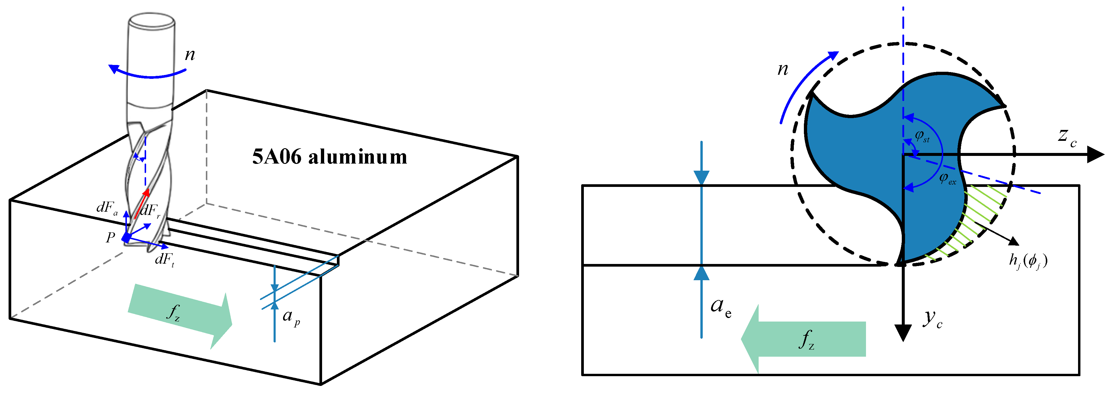
Robotic milling force analysis is identical to that for five-axis machine tool milling, as milling force modeling utilizes the tool’s cutting conditions and characteristics while partially excluding machine-specific properties. Based on the instantaneous rigid mechanical modeling approach, as illustrated in Figure 1, the milling cutter cutting edge is discretized axially into finite identical micro-segments P. $d{F}_t$, $d{F}_r$, and $d{F}_a$ represent the tangential, radial, and axial milling force components on micro-segment P in the local coordinate system, respectively.

Instantaneous cutting thickness refers to the radial distance between the cutting path of the current cutting edge and the preceding cutting edge at the instantaneous contact angle, ${\varphi }_j$, representing the instantaneous undeformed chip thickness between two adjacent cutting edges, as given by Equation (1).

$$h_j\left({\varphi }_j\right)=f_z\sin {\varphi }_j$$

(1)

where $f_z$ denotes the feed per tooth. The milling force components acting on any micro-segment of the j-th cutting edge are expressed in summation form: the product of shearing force coefficients with instantaneous cutting thickness and element axial depth of cut, plus the product of plowing force coefficients with the element axial depth of cut.

$$\begin{array}{l}d{F}_{t,j}\left({\varphi }_j\right)=K_{tc}{h}_j\left({\varphi }_j\right)\cdot d{a}_p+K_{te}\cdot d{a}_p\\ d{F}_{r,j}\left({\varphi }_j\right)=K_{rc}{h}_j\left({\varphi }_j\right)\cdot d{a}_p+K_{re}\cdot d{a}_p\\ d{F}_{a,j}\left({\varphi }_j\right)=K_{ac}{h}_j\left({\varphi }_j\right)\cdot d{a}_p+K_{ae}\cdot d{a}_p\end{array}$$

(2)

where $d{F}_{t,j}\left({\varphi }_j\right)$ denotes tangential micro-segment milling force, $d{F}_{r,j}\left({\varphi }_j\right)$ denotes radial micro-segment milling force, and $d{F}_{a,j}\left({\varphi }_j\right)$ denotes axial micro-segment milling force. $K_{tc}$, $K_{rc}$, and $K_{ac}$ are tangential, radial, and axial shearing force coefficients, $K_{te}$, $K_{re}$, and $K_{ae}$ are tangential, radial, and axial plowing force coefficients, and $d{a}_p$ represents the axial depth of cut of the micro-segment.

The average milling force, $\stackrel{\_\_\_}{F_q}$, per tooth cycle is obtained by integrating over one spindle revolution and dividing by the tooth engagement angle, ${\varphi }_p$ [34].

$$\left\{\begin{array}{l}\stackrel{\_\_\_}{F_q}={\displaystyle \frac{1}{{\varphi }_p}}{\displaystyle {\int }_{{\varphi }_{st}}^{{\varphi }_{ex}}d{F}_q\left({\varphi }_j\right)\cdot d{a}_p;q=1,2,3}\\ {\varphi }_p={\displaystyle \frac{2\pi }{N}}\end{array}\right.$$

(3)

where ${\varphi }_{st}$ and ${\varphi }_{ex}$ denote the instantaneous engagement angle upper and lower bounds of the helical flute contact zone, respectively. N represents the number of tool teeth.

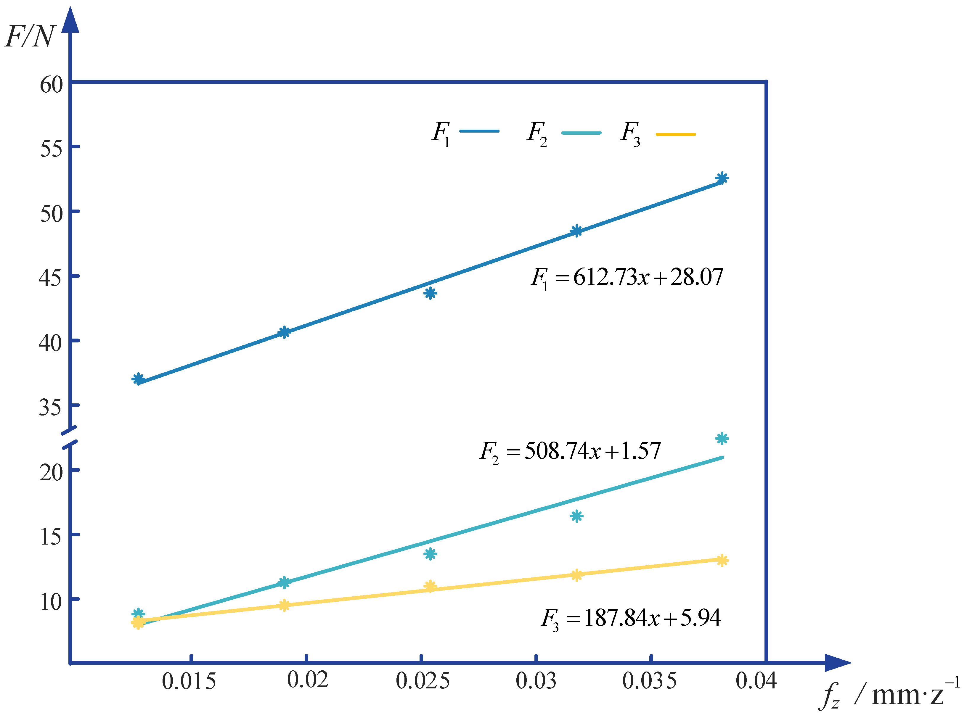
Milling experiments were conducted at fixed engagement angles and axial depths of cut while varying only the feed rate [35]. Due to the weak stiffness characteristics of robots, full-slot milling readily induces chatter, significantly impacting cutting force measurements. Therefore, a half-slot milling approach was adopted. The average force can be expressed as the sum of a linear function of the feed rate and the edge force.

2.2. Identification of Cutting Force Coefficients

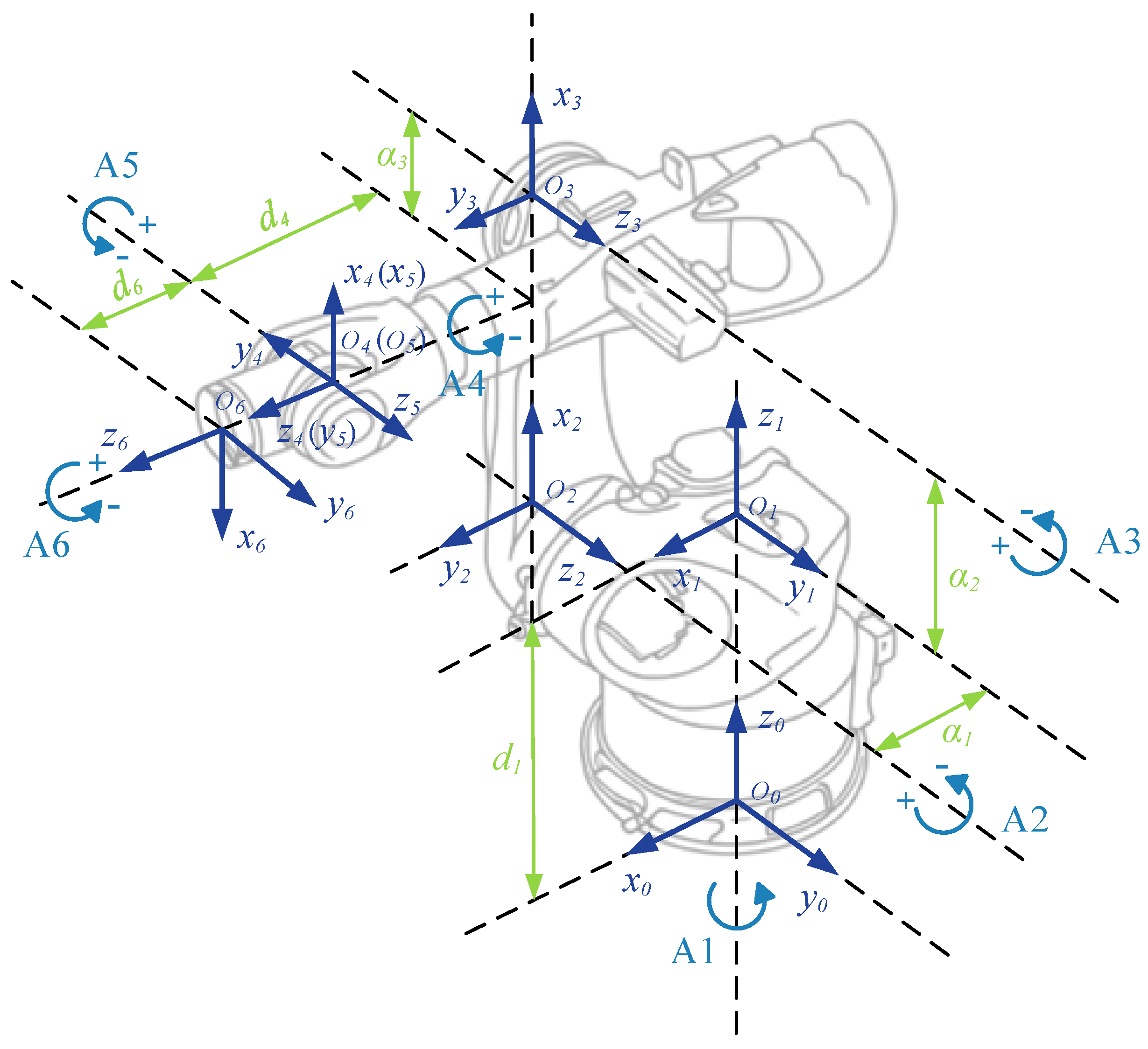
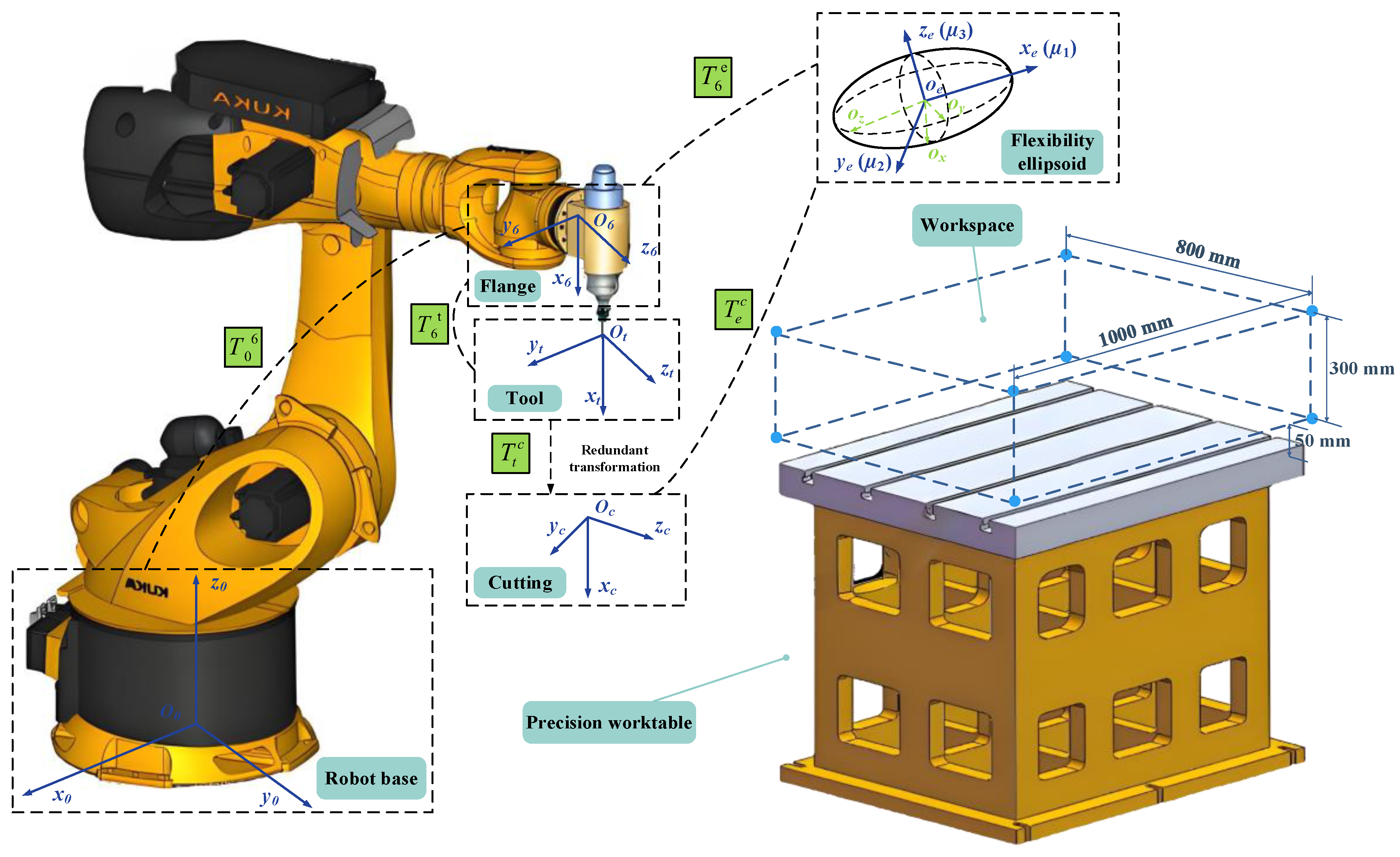
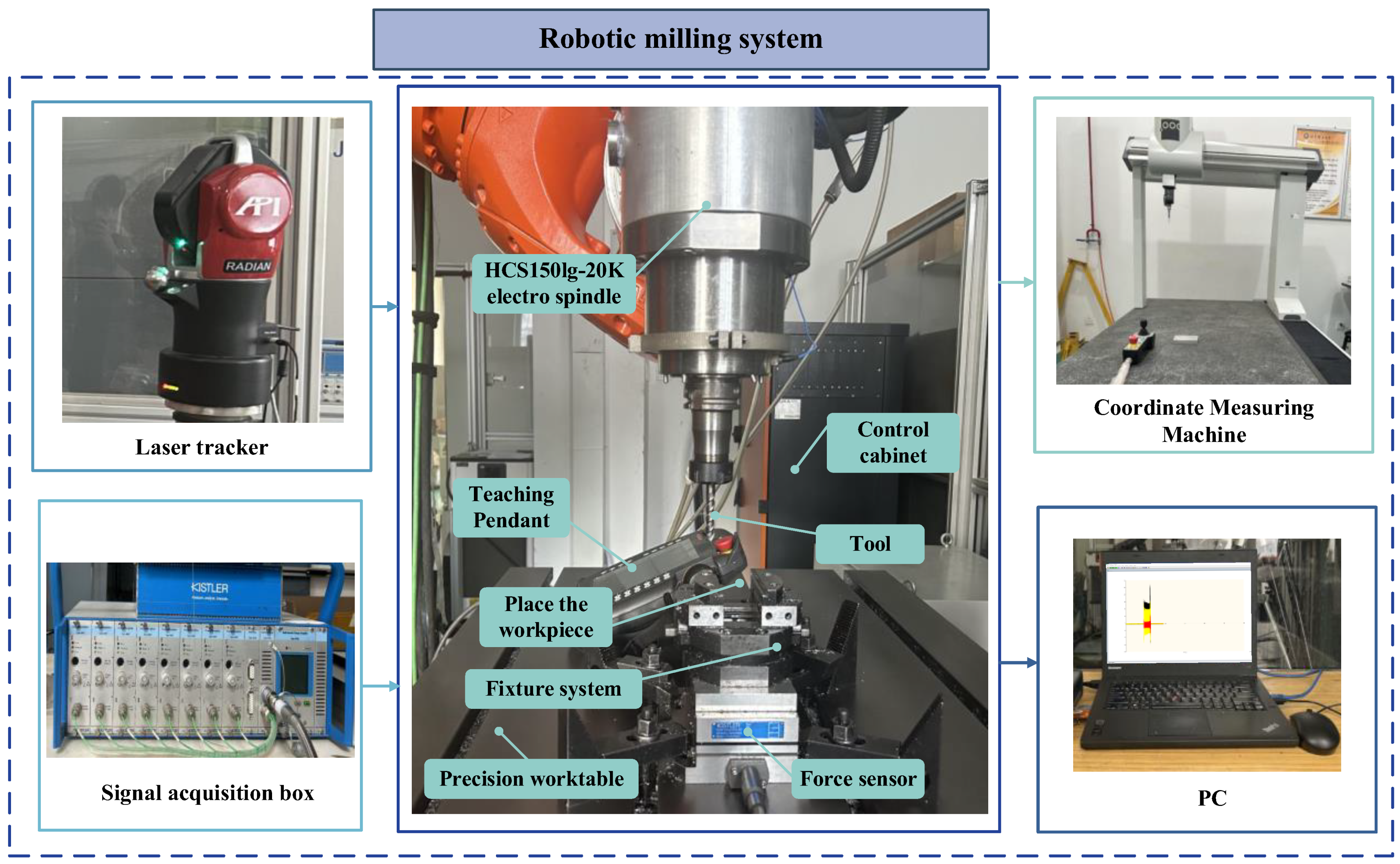
In this study, all the research contents, including the stiffness model and experiments, are carried out on a six-axis robot milling platform based on a KUKA KR 600 R2830 robot. The kinematic model of the 6 -DOF industrial robot is illustrated in Figure 2. The parameters of the revised MDH model are shown in

Table 1. Revised MDH model parameters of KUKA KR 600 R2830 robot.

Rob	Axis	${\mathit{a}}_{\mathit{i}-1}$ (mm)	${\mathit{a}}_{\mathit{i}-1}$ (°)	${\mathit{d}}_{\mathit{i}}$ (mm)	${\mathit{\theta }}_{\mathit{i}}$ (°)	$\left[{\mathit{\theta }}_{\mathbf{i}\mathbf{min}},{\mathit{\theta }}_{\mathbf{i}\mathbf{max}}\right]$ (°)
1	A1	0	0	1045	$-{\theta }_1$	$\left[-185,185\right]$
2	A2	500	−90	0	${\theta }_2$	$\left[-130,20\right]$
3	A3	1300	0	0	${\theta }_3-90$	$\left[-100,144\right]$
4	A4	−55	−90	1025	$-{\theta }_4$	$\left[-350,350\right]$
5	A5	0	90	0	${\theta }_5$	$\left[-120,120\right]$
6	A6	0	−90	290	$-180-{\theta }_6$	$\left[-350,350\right]$

. Based on actual process constraints, the rotation range of Joint 2 is set to [−120°, −30°]. The robotic base coordinate system is $o_0-x_0{y}_0{z}_0$ and the flange coordinate system is $o_6-x_6{y}_6{z}_6$. The determination of the transformation matrix, $T_0^6$, from $o_0-x_0{y}_0{z}_0$ to $o_6-x_6{y}_6{z}_6$ is accomplished by the MDH model. The HCS150lg-20K electric spindle installed on the robot EE and the integral end mill give it the ability of milling.

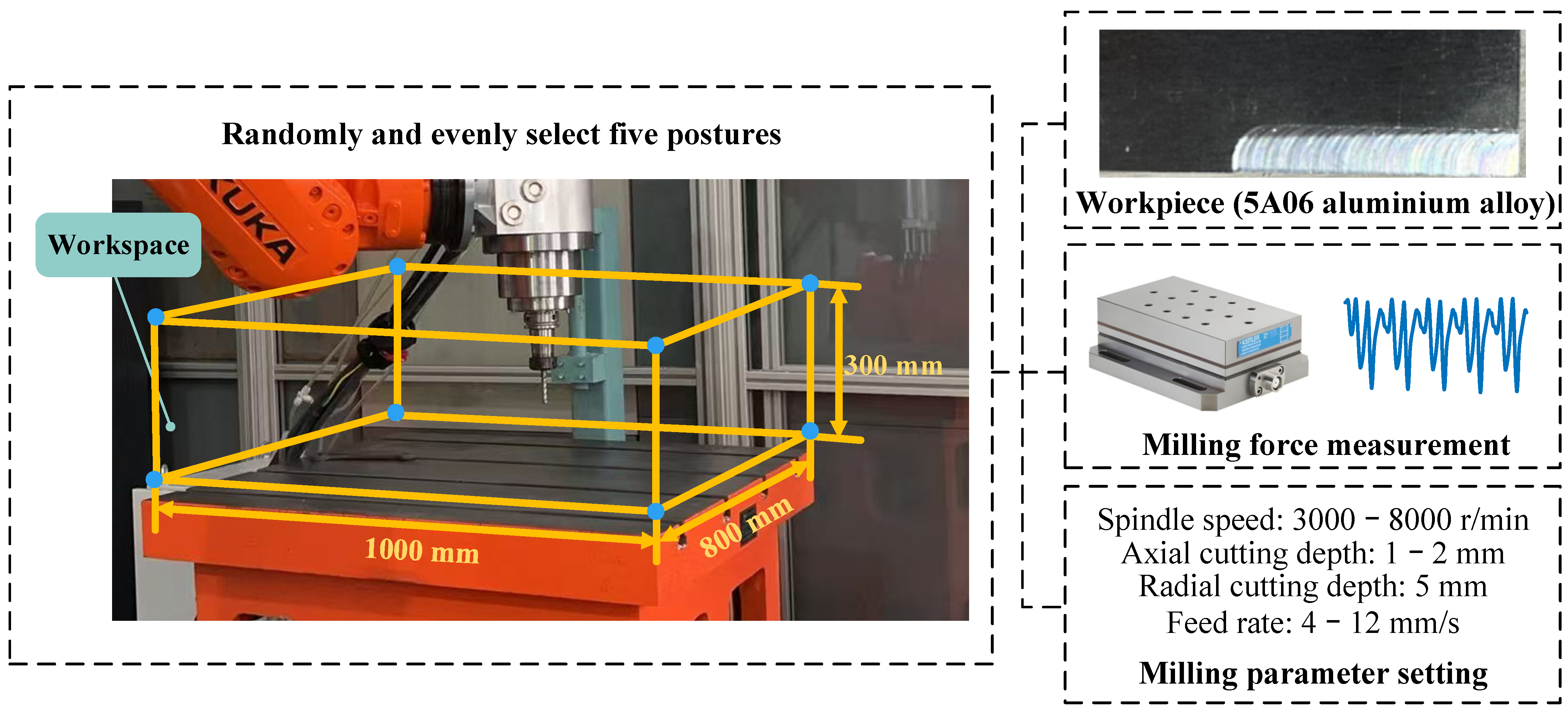
As shown in Figure 3, the actual x, y, and z working range was determined to be within the robot base coordinate system $o_0-x_0{y}_0{z}_0$ [−130 mm, 870 mm], [1800 mm, 2600 mm] and [1000 mm, 1300 mm], considering the height of the fixture, the commonly used milling position and the relative position between the precision workbench and the robot. Within this workspace, five positions are randomly and uniformly selected for milling experiments, where each position corresponds to a distinct robot posture. They are distributed at the four corners and the inner center to ensure that the posture change amplitude is as large as possible and covers the workspace. The machining in this study was performed using a three-flute carbide end mill on 5A06 aluminum alloy. The tool had a diameter of 10 mm and a helix angle of 45 degrees. The tool overhang was kept constant at 60 mm.

Taking the parameters in

Table 2. Actual milling parameters under posture 1.

Number	Spindle Speed n (r/min)	Radial Cutting Depth ae (mm)	Axial Cutting Depth ap (mm)	Feed Speed Vf (mm/s)
1	6333	5	2	4
2	6333	5	2	6
3	6333	5	2	8
4	6333	5	2	10
5	6333	5	2	12
6	4667	5	1	4
7	4667	5	1	6
8	4667	5	1	8
9	4667	5	1	1
10	4667	5	1	12

as an example, for a specified posture, two sets of cutting force identification experiments were conducted under dry-cutting conditions. Climb milling (down milling) is employed in this study, as the chip thickness gradually decreases from the start of the cut. Its process generates downward-oriented cutting forces, resulting in stable machining conditions, lower power consumption, and reduced cutting deformation. It is therefore well-suited for machining aluminum alloys of low hardness and for use with industrial robot systems exhibiting weak stiffness. The cutting parameters were randomly and evenly selected within the ranges of spindle speed n (3000–8000 r/min), feed rate V_f (4–12 mm/s), and axial cutting depth a_p (1–2 mm). Triaxial milling forces were measured by a Kistler 9257B piezoelectric dynamometer fixed to the workpiece, with a sampling frequency of 10,240 Hz. High-frequency noise components were removed via a 2000 Hz low-pass filter.

The cutting force measurement results of the experimental groups numbered 1–5 are shown in Figure 4.

The cutting force coefficient identification results are shown in

Table 3. Identification results of milling force coefficient.

Posture	n (r/min); ap (mm)	${\mathit{K}}_{\mathit{t}\mathit{c}}$ (N/mm2)	${\mathit{K}}_{\mathit{t}\mathit{e}}$ (N/mm)	${\mathit{K}}_{\mathit{r}\mathit{c}}$ (N/mm2)	${\mathit{K}}_{\mathit{r}\mathit{e}}$ (N/mm)	${\mathit{K}}_{\mathit{a}\mathit{c}}$ (N/mm2)	${\mathit{K}}_{\mathit{a}\mathit{e}}$ (N/mm)
1	6333; 2	852.65	15.30	−273.55	−13.65	196.69	3.96
	4667; 1	858.98	15.12	−276.81	−13.93	195.79	3.72
2	6333; 1.5	856.07	15.02	−273.97	−13.36	191.50	4.76
	3000; 2	850.49	15.71	−272.99	−13.87	194.12	3.98
3	6333; 1.5	855.27	15.15	−275.70	−13.25	196.25	3.88
	4667; 1	854.33	15.62	−275.08	−14.20	194.02	3.01
4	6333; 1	855.61	15.26	−272.32	−14.28	196.19	4.61
	8000; 1.5	851.44	16.80	−277.87	−14.13	194.52	4.13
5	3000; 2	852.54	15.19	−277.44	−14.63	195.14	3.73
	8000; 1.5	852.46	15.87	−277.85	−14.65	192.89	4.39

. It is evident that, when ignoring signal acquisition errors, the cutting force coefficients exhibit minor variations but remain within acceptable bounds during stable milling of identical workpiece material with a specific tool under multiple postures and various machining parameters. Thus, for the robotic milling system used in this study, altering robot postures and milling parameters does not exert a significant impact on the milling force coefficients.

2.3. Milling Force Prediction and Experimental Verification

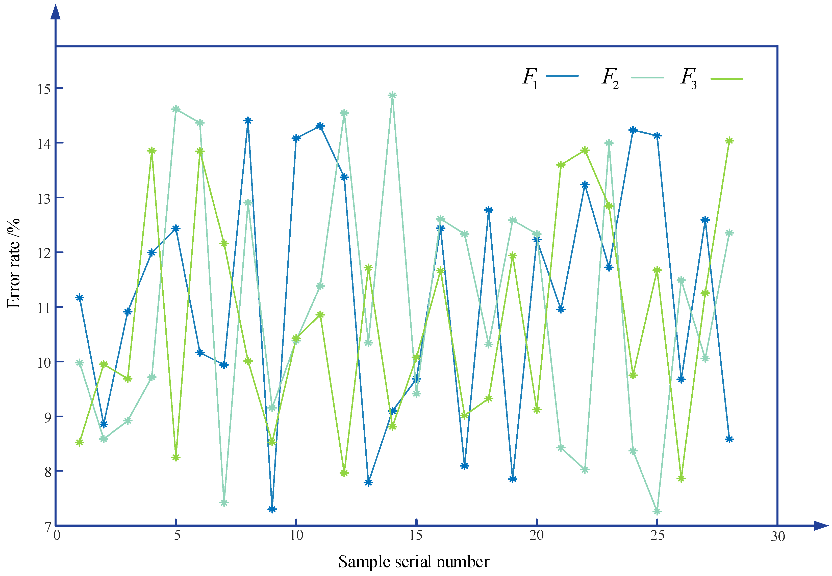
Based on the averaged cutting force coefficients identified in Section 2.2, predictions for milling forces under different parameters were made using various instantaneous engagement angles in helical flute contact zones. The validation set comprised 16 sets of four-factor four-level orthogonal experiments under posture 1 with cutting parameters randomly and evenly selected within the range of spindle speed (3000–8000 r/min), feed rate (6–12 mm/s), axial cutting depth a_p (1–2 mm), and radial cutting depth a_e (0.5–5.5 mm) and 12 sets of supplementary experiments at four additional postures with cutting parameters randomly selected within the orthogonal parameter ranges. Prediction error rates are shown in Figure 5.

In summary, when robot postures and milling parameters vary, the complex static and dynamic characteristics of the robot alter the instantaneous material removal rate, thereby influencing cutting force coefficients and the accuracy of cutting force predictions. However, this influence remains within acceptable bounds. The established milling force model demonstrates reasonably high prediction accuracy and is capable of describing milling force variations during robotic milling operations.

3. Stiffness Model and Stiffness Performance Index

3.1. The Stiffness Model of Robot

The robotic arm, connecting plate, and electric spindle constitute the primary components of the milling system in this study. Their load-bearing capacity directly influences cutting performance. Furthermore, the connecting plate, fabricated from high-strength material with a compact structure, exhibits exceptionally high stiffness. The stiffness of the electric spindle primarily depends on the structural characteristics of its internal shaft and bearings, typically on the order of 50 N/µm. Thus, to simplify the stiffness analysis of the milling system, the following assumptions are made: (1) the robot is considered the sole source of deformation and (2) cutting loads are rigidly transmitted sequentially and ultimately act at the center of the robot flange. The overall stiffness of the machining system is determined by the robot stiffness and is predominantly governed by the machining posture.

The Cartesian stiffness matrix of the robot is expressed as

$$K=J^{-T}(K_{\theta }-K_c)J^{-1}$$

(4)

where $K$ is the end stiffness matrix. $J$ is the Jacobian matrix under $o_0-x_0{y}_0{z}_0$ and $K_{\theta }$ is a 6 × 6 diagonal matrix representing the spatial stiffness of the robot. The complementary stiffness matrix is typically neglected when the load is significantly lighter than the payload capacity and the robot exhibits good maneuverability [12].

By adjusting counterweights, total forces of 600 N, 800 N, 1000 N, and 1200 N were applied, as shown in Figure 6. Using a laser tracker, a spatial vector between the force application point and fixed pulley 1 was established to derive three-dimensional forces under respective loads. Coordinates of measurement points were recorded under unloaded and different loaded states to calculate deformation. Combined with previous work [36], the calculated $K_{\theta }$ can effectively indicate the carrying capacity of the robot in any posture.

$$K_{\theta }=diag\left[6.982,6.461,3.684,2.721,1.595,2.024\right]\times {10}^6 \mathrm{N}\cdot \mathrm{m}/\mathrm{r}\mathrm{a}\mathrm{d}$$

(5)

3.2. Stiffness Performance Evaluation Index

Combining the robot Cartesian compliance matrix, $C$, with the relationship between the force acting on the EE and the resulting generalized deformation, $\mathrm{\Delta }x$, yields:

$$\mathrm{\Delta }x=\left[\begin{array}{c}\mathrm{\Delta }{x}_t\\ \mathrm{\Delta }{x}_r\end{array}\right]=CF=K^{-1}F=J{K}_{\theta }^{-1}{J}^{\mathrm{T}}F=\left[\begin{array}{cc}{c}_{fd}& c_{f\delta }\\ c_{md}& c_{m\delta }\end{array}\right]F$$

(6)

where $c_{fd}$ is the force–linear displacement compliance matrix, $c_{f\delta }$ is the force–angular displacement compliance matrix, $c_{md}$ is the moment–linear displacement compliance matrix, $c_{m\delta }$ is the force–linear displacement compliance matrix, and $\mathrm{\Delta }{x}_t$ and $\mathrm{\Delta }{x}_r$ denote the translational and rotational deformation vectors of the EE, respectively.

In the milling process, the main factor affecting the machining quality is the linear displacement deformation of the cutting tool, so the torque applied on EE is ignored. Equation (6) can thus be simplified as Equation (7):

$$\mathrm{\Delta }{x}_t=c_{fd}F$$

(7)

A compliance ellipsoid is constructed, with the square roots of the matrix $c_{fd}{}^{\mathrm{T}}c_{fd}$ eigenvalues ${\lambda }_1$, ${\lambda }_2$, and ${\lambda }_3$ as the semi-principal axis lengths and the eigenvector directions ${\mu }_1$, ${\mu }_2$, and ${\mu }_3$ as the principal axes.

During milling tasks, the robot system achieves spatial position description and control by establishing collaborative relationships between local coordinate systems of components. As shown in Figure 7, the following coordinate systems are defined:

• Ellipsoidal coordinate system $o_e-x_e{y}_e{z}_e$: The origin $o_e$ is located at the center of the robot flange, with the $x_e$ axis, $y_e$ axis, and $z_e$ axis directions being the eigenvector directions ${\mu }_1$, ${\mu }_2$, and ${\mu }_3$.
• Tool coordinate system $o_t-x_t{y}_t{z}_t$: The origin $o_t$ is located at the end of the tool. The $x_t$-axis coincides with the cutter axis vector. The $y_t$-axis is in the same direction as the $y_6$-axis of the flange coordinate system.
• Cutting coordinate system $o_c-x_c{y}_c{z}_c$: The origin $o_c$ and $x_c$-axis coincides with the tool coordinate system, and the positive direction of $z_c$-axis coincides the feed direction.

The center of this ellipsoid coincides with the end-flange center. Its posture varies with the robot’s posture changes and serves to quantitatively evaluate the robot resistance to deformation at a given posture. Specifically, shorter semi-axis lengths formed between the ellipsoid surface and center $o_e$ indicate higher stiffness when operating along that direction.

A fixed installation posture exists between the tool holder, electric spindle, connecting plate, and end flange. Thus, after determining the tool overhang, the coordinate transformation relationship $T_6^t$ between $o_6-x_6{y}_6{z}_6$ and $o_t-x_t{y}_t{z}_t$ remains constant and can be calibrated based on the mechanical interfaces between intermediate components. Since the three-dimensional column vectors ${\mu }_1,{\mu }_2$ and ${\mu }_3$ denote the direction cosine parameters of the three coordinate axes ($x_e$, $y_e$ and ${\mathrm{z}}_e$) in $o_6-x_6{y}_6{z}_6$. Attitude matrix $T_6^e$ between $o_e-x_e{y}_e{z}_e$ and $o_6-x_6{y}_6{z}_6$ can be described.

At the same time, $o_c-x_c{y}_c{z}_c$ and $o_t-x_t{y}_t{z}_t$ have a rotation relationship, $T_t^c$ determined by redundancy angle ${\gamma }_{\mathrm{i}}$. When further combining with $T_6^t$ and $T_6^e$, matrix $T_e^c$, which describes the relationship between $o_e-x_e{y}_e{z}_e$ and $o_c-x_c{y}_c{z}_c$, is formed.

$$T_{\mathrm{e}}^c={\left(T_6^{\mathrm{e}}\right)}^{-1}{T}_6^{\mathrm{t}}{T}_t^c$$

(8)

The milling force direction, $e_f$, is expressed in the cutting coordinate system $o_c-x_c{y}_c{z}_c$, so flexibility indices $‖o_e{o}_1‖$, $‖o_e{o}_2‖$, and $‖o_e{o}_3‖$ in the actual load direction can be calculate.

$$\begin{array}{c}‖o_e{o}_1‖=\sqrt{{\displaystyle \frac{1}{\frac{e_{f_{1,1}}^2}{{\lambda }_1^2}+\frac{e_{f_{1,2}}^2}{{\lambda }_2^2}+\frac{e_{f_{1,3}}^2}{{\lambda }_3^2}}}}\\ ‖o_e{o}_2‖=\sqrt{{\displaystyle \frac{1}{\frac{e_{f_{2,1}}^2}{{\lambda }_1^2}+\frac{e_{f_{2,2}}^2}{{\lambda }_2^2}+\frac{e_{f_{2,3}}^2}{{\lambda }_3^2}}}}\\ ‖o_e{o}_3‖=\sqrt{{\displaystyle \frac{1}{\frac{e_{f_{3,1}}^2}{{\lambda }_1^2}+\frac{e_{f_{3,2}}^2}{{\lambda }_2^2}+\frac{e_{f_{3,3}}^2}{{\lambda }_3^2}}}}\end{array}$$

(9)

The stiffness coupling effects are negligible, given the use of industrial robot in this research with high payload capacity for milling relatively soft aluminum alloy workpieces. Consequently, machining accuracy is primarily addressed in the milling plane normal direction and path lateral direction, focusing exclusively on $‖o_e{o}_2‖$ and $‖o_e{o}_3‖$.

During milling, periodic dynamic milling forces act on the EE. These forces can always be decomposed into components along the feed direction, perpendicular to the feed direction, and the axial direction. A direct proportional relationship is assumed between the EE’s translational displacement and the force applied in the same direction. The industrial robot used possesses six joint angles, granting the milling system six degrees of freedom. The rotational degree of freedom, $\gamma$, around the tool axis is redundant for five-axis machining. By optimizing the robot’s stiffness performance, the optimal redundancy angle, ${\gamma }_{\mathrm{i}}$, can be obtained, after which joint angles are resolved through inverse kinematics.

Within the workspace, the variation patterns of $‖o_e{o}_2‖$ and $‖o_e{o}_3‖$ with the actual machining posture are complex and lack precise quantitative relationships. As shown in

Table 4. Variation in flexibility indices in different positions.

Posture	$‖{\mathit{o}}_{\mathit{e}}{\mathit{o}}_2‖$ (10−7 m/N)	$‖{\mathit{o}}_{\mathit{e}}{\mathit{o}}_3‖$ (10−7 m/N)
$150 \mathrm{mm}, 1830 \mathrm{mm}, 1100 \mathrm{mm}, {\gamma }_{\mathrm{i}}={32}^{\circ }$	3.879	4.141
$550 \mathrm{mm}, 1830 \mathrm{mm}, 1100 \mathrm{mm}, {\gamma }_{\mathrm{i}}={32}^{\circ }$	4.194	3.646

, when the robot transitions from posture (150 mm, 1830 mm, 1100 mm, ${\gamma }_{\mathrm{i}}={32}^{\circ }$) to posture (550 mm, 1830 mm, 1100 mm, ${\gamma }_{\mathrm{i}}={32}^{\circ }$), both the magnitude and trend of changes in $‖o_e{o}_2‖$ and $‖o_e{o}_3‖$ differ. To comprehensively address machining accuracy in both the milling plane normal direction and path lateral direction, appropriate weighting factors must be assigned. This is achieved by introducing milling forces $F_2$ and $F_3$ along corresponding directions to represent deformations under actual cutting load orientations. The comprehensive stiffness performance index $C_{sf}=C_s+C_f=‖o_e{o}_2‖\cdot F_2+‖o_e{o}_3‖\cdot F_3$ is defined such that a smaller value indicates superior stiffness performance.

4. Robot Posture Optimization Model and Algorithm

4.1. Stiffness Index Verification Experiment

Prior to the experimental investigation of posture optimization, it is essential to validate the effectiveness of the proposed stiffness index.

In order to ensure the smooth progress of the milling process, first of all, it is necessary to ensure that the robot joint angle is within the constraint range and away from the joint limit position, so as to avoid the occurrence of stop points, which will lead to the obvious shaking of the processing system and damage to the workpiece.

$$L_{\mathrm{a}}={\displaystyle \frac{1}{6}}{\displaystyle \sum _{i=1}^6\frac{{\left({\theta }_{\mathrm{i}\min }-{\theta }_{\mathrm{i}\max }\right)}^2}{8}}\cdot \left[{\displaystyle \frac{1}{{\left({\theta }_{i\min }-{\theta }_{\mathrm{i}}\right)}^2}}+{\displaystyle \frac{1}{{\left({\theta }_{\mathrm{i}\max }-{\theta }_i\right)}^2}}\right]$$

(10)

where $L_a\in [1,+\infty )$ is the relationship between the current joint angle and the joint limit. The closer its value is to 1, the further it is from the joint limit position.

Additionally, proximity to singular configurations must be avoided to eliminate collision risks. The reciprocal of the normalized Jacobian condition number $L_{\mathrm{b}}\in (0,1]$ quantifies the distance between the current posture and singular points. The closer its value is to 1, the further it is from the singular point.

$$L_{\mathrm{b}}={\displaystyle \frac{6}{\sqrt{tr\left(J_N{J}_N^{\mathrm{T}}\right)tr\left[{\left(J_N{J}_N^{\mathrm{T}}\right)}^{-1}\right]}}}$$

(11)

where $J_N=\left[\begin{array}{cc}{\displaystyle \frac{1}{L}}{I}_{3\times 3}& 0_{3\times 3}\\ 0_{3\times 3}& I_{3\times 3}\end{array}\right]J$, and L is the characteristic length of the robot.

As shown in Figure 8, verification experiments were conducted. The same tool, workpiece material, force signal sampling rate, and filtering method from Section 2 force coefficient identification experiments were employed. To amplify observable effects, milling parameters listed in

Table 5. Milling experimental parameters.

Number	n (r/min)	ae (mm)	ap (mm)	Vf (mm/s)
1	3000	5	2	10
2	5000	4.5	1.5	8
3	7000	5.5	2	12

were used to generate relatively large milling forces. Within the workspace, three arbitrary positions were selected: position 6: (550 mm, 1830 mm, 1100 mm); position 7: (−50 mm, 2230 mm, 1120 mm); and position 8: (250 mm, 2030 mm, 1050 mm). The robot was preset to a redundancy angle of 0°. Considering constraints of joint limit boundaries and singular configurations, the redundancy angle domain is non-continuous. An exhaustive search over 0–360° was performed to identify the minimum value of the proposed index, $C_{sf}$.

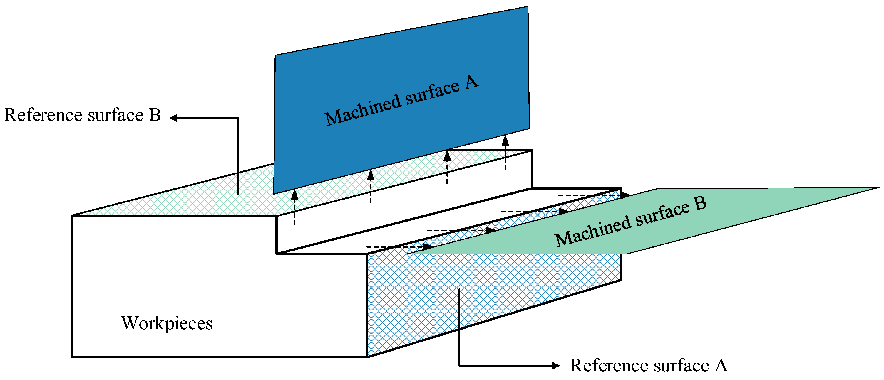
Reference planes A and B represent the finish-machined surfaces. The measurement surface was obtained through a single milling path. Consequently, the machining error, $d_A$ and $d_B$, can be defined as the deviation between the normal distance separating the two surfaces and the actual set parameters. Points were uniformly sampled on both surfaces using a coordinate measuring machine (CMM), and the surfaces were reconstructed to quantify errors, as shown in Figure 9. The purpose of the measurement is to ensure good agreement between the actual depth and width of cut and their prescribed values, thereby avoiding variations in milling forces caused by an abnormal increase in the material removal rate (MRR). Such variations would induce severe robot vibration and potentially lead to a more pronounced hardening layer [37], adversely affecting the machining quality, service performance, or re-machinability of the processed surface.

As shown in

Table 6. Under setting milling parameter 1, the measurement results $d_A$ and $d_B$.

	Milling Parameter 1				${\mathit{\gamma }}_{\mathbf{i}}$ (°)
Posture	${\mathit{C}}_{\mathit{f}}$ (10−6 m)	${\mathit{C}}_{\mathit{s}}$ (10−6 m)	${\mathit{d}}_{\mathit{A}}$ (mm)	${\mathit{d}}_{\mathit{B}}$ (mm)	${\mathit{\gamma }}_{\mathbf{i}}$
6	8.543	12.396	0.051	0.069	38
7	12.822	22.063	0.072	0.091	358
8	9.268	17.174	0.056	0.082	20

,

Table 7. Under setting milling parameter 2, the measurement results $d_A$ and $d_B$.

	Milling Parameter 2				${\mathit{\gamma }}_{\mathbf{i}}$ (°)
Posture	${\mathit{C}}_{\mathit{f}}$ (10−6 m)	${\mathit{C}}_{\mathit{s}}$ (10−6 m)	${\mathit{d}}_{\mathit{A}}$ (mm)	${\mathit{d}}_{\mathit{B}}$ (mm)
6	5.233	9.006	0.035	0.053	41
7	7.549	16.199	0.045	0.079	358
8	5.542	12.55	0.037	0.071	20

and

Table 8. Under setting milling parameter 3, the measurement results $d_A$ and $d_B$.

	Milling Parameter 3				${\mathit{\gamma }}_{\mathbf{i}}$ (°)
Posture	${\mathit{C}}_{\mathit{f}}$ (10−6 m)	${\mathit{C}}_{\mathit{s}}$ (10−6 m)	${\mathit{d}}_{\mathit{A}}$ (mm)	${\mathit{d}}_{\mathit{B}}$ (mm)
6	5.052	7.463	0.032	0.044	35
7	9.386	13.411	0.056	0.075	111
8	7.215	10.013	0.060	0.057	17

no significant deviation exists between the actual machined plane and reference plane, with close alignment between actual and set values, demonstrating the effectiveness of the posture accuracy compensation method. For three distinct milling parameter sets, the actual error and proposed index exhibit identical variation trends with an approximate proportional relationship. This confirms the capability of the proposed index to represent stiffness performance in the actual cutting direction. At the same time, it can be concluded that under the same position and different milling parameters, the values of $C_f$ and $C_s$ are different, and the optimal redundant angle, ${\gamma }_{\mathrm{i}}$, may also be different. For a certain processing position, targeted optimization should be carried out in combination with the setting of milling parameters.

Additionally, further discussion compares optimizing only $C_f$, optimizing only $C_s$, and optimizing $C_{sf}$, using posture 6 and milling parameter 1 as an example. As shown in

Table 9. $C_f$ and $C_s$ under different optimization objectives.

Condition	Posture 6; Milling Parameter 1
	${\mathit{C}}_{\mathit{f}}$ (10−6 m)	${\mathit{C}}_{\mathit{s}}$ (10−6 m)
Min $C_f$	8.394	13.068
Min $C_s$	9.746	11.934
Min $C_{sf}$	8.543	12.396

, when exclusively optimizing either $C_f$ or $C_s$ alone, the other exhibits a significant increase. When comprehensively optimizing $C_{sf}$, both of them achieve favorable optimization outcomes.

4.2. Establishment of Optimization Model

As established in Section 4.1, the proposed index effectively reflects robotic stiffness performance. Therefore, for large-range continuous milling tasks along specified tool paths, the path can be discretized into $M$ segments per Equation (12) to achieve globally optimal average stiffness.

$$\begin{gathered} (p_{start},p_{start}+1\cdot m,p_{start}+2\cdot m,\dots ,p_{start}+(M-1)\cdot m,\dots ,p_{over}) \\ m={\displaystyle \frac{(p_{start}-p_{over})}{M}} \end{gathered}$$

(12)

where $p_{start}$ is the starting position of the path, $p_{over}$ is the end position of the path, and $m$ is the distance between discrete points. Since the movement of the robot between the discrete CL points needs to ensure smoothness, constraints in Equation (13) are introduced.

$$|{\theta }_i-{\theta }_{i-1}|\le \delta {\omega }_{\max }\mathrm{\Delta }t$$

(13)

where ${\theta }_i$ and ${\theta }_{i-1}$ are the joint angles corresponding to the $i$ th CL point and the $i$-1th CL point, respectively; $\delta \in (0,1]$ is the coefficient of motion smoothness. ${\omega }_{\max }$ is the maximum angular velocity corresponding to the robot six joints. $\mathrm{\Delta }t$ is the time taken to move a distance of $m$, which is calculated based on the actual feed rate.

In conclusion, the robot posture optimization model can be established.

$$\left\{\begin{array}{c}min{\displaystyle \sum _{i=1}^{M+1}{K}_{\mathrm{sf}}}\\ s.t.{\theta }_i=f^{-1}({\gamma }_i)\\ {\theta }_{min}\le {\theta }_i\le {\theta }_{max}\\ \left|{\theta }_i-{\theta }_{i-1}\right|\le \delta {\omega }_{max}\mathrm{\Delta }t\\ \begin{array}{l}{L}_{\mathrm{a}}<{\epsilon }_1\\ L_{\mathrm{b}}>{\epsilon }_2\end{array}\end{array}\right.$$

(14)

where $f^{-1}$ denotes the inverse solution of the robot kinematics. ${\epsilon }_1$ and ${\epsilon }_2$ are the constraint values, which are given by the operator.

4.3. Posture Optimization Based on Dynamic Programming

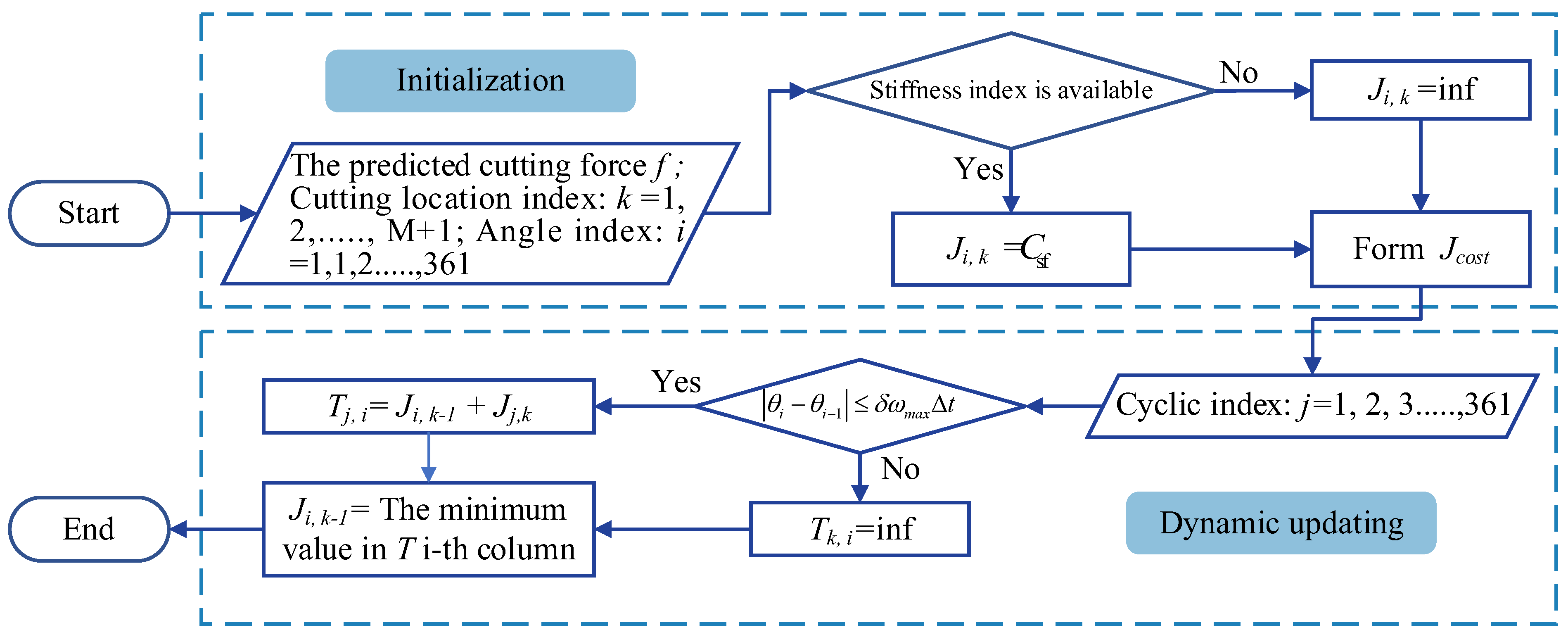
Constrained by robot kinematics, single-step optimization strategies readily trap solutions in local optima, impeding the attainment of the global trajectory optimum. The dynamic programming approach, employed to solve shortest-path problems from start to target nodes, constructs a node graph with redundancy angle ${\gamma }_{\mathrm{i}}$ as the vertical axis and CL point count as the horizontal axis. Here, elements in loss matrix $J_{\cos t}$ correspond to nodes, as depicted in Figure 10. To identify the milling path with optimal average stiffness, the optimization procedure follows Figure 11.

Specifically, the loss matrix is dynamically updated with the objective of minimizing the total flexibility coefficient of each CL point, under the constraints given by the robot attitude optimization model mentioned above, which is a reverse process. First, initialize loss matrix $J_{\cos t}$ with rows equal to the number of discrete trajectory points and columns equal to the number of discrete redundancy angles (1° resolution). For a specific discrete point position and redundancy angle, compute proposed index $C_{sf}$ and populate loss matrix $J_{\cos t}$; if computation is infeasible due to joint limit constraints, set the value to ∞. Second, starting from the path endpoint, take element (i, k − 1) in the matrix $J_{\cos t}$, sum it individually with all elements in column k, and calculate column vector $T_{j,i}$. If constraints prevent the ability to reach a node, set the sum to ∞. Update element (i, k − 1) in $J_{\cos t}$ with the minimum sum obtained in $T_{j,i}$, representing the minimum total $C_{sf}$ from position (i, k − 1) to the trajectory endpoint. After processing all rows in column k − 1 of loss matrix $J_{\cos t}$, the algorithm iteratively proceeds to the preceding column. This backward recursion continues stepwise toward the path start point, ultimately yielding the global minimum total sum of $C_{sf}$. That is, the value at the first row and first column of the updated loss matrix $J_{\cos t}$ represents the minimum total $C_{sf}$ sum from starting at the first discrete point with a redundant angle of 360° to the end of the path trajectory.

The actual redundant angle sequence is determined through a forward retrieval process. The value at the corresponding position in the initialized $J_{\cos t}$ is subtracted from that in the updated $J_{\cos t}$. The resulting difference is then compared to the values in the next column of the updated $J_{\cos t}$ to identify the matching entry, from which the redundant angle for the subsequent CL point is obtained.

The milling path is selected from (200 mm, 2000 mm, 1100 mm) to (200 mm, 2400 mm, 1100 mm) using milling parameter 1 in Table 5. Assuming negligible robot stiffness variation within 10 cm ranges and adequate compensation of positioning errors, no significant path deviation occurs over the 40 cm milling span. Divide the milling path into four parts equally. Milling forces are calculated via the coefficients identified in Section 2. The resulting redundancy angle sequences were calculated in

Table 10. Optimized redundant angle sequence.

	${\mathit{\gamma }}_1$ (°)	${\mathit{\gamma }}_2$ (°)	${\mathit{\gamma }}_3$ (°)	${\mathit{\gamma }}_4$ (°)	${\mathit{\gamma }}_5$ (°)	${\mathit{C}}_{\mathit{s}\mathit{f}}$ (10−4 m)
Single-step optimization	15	13	11	9	6	1.6150
Dynamic programming	253	253	254	254	259	1.4208

. Both single-step optimization and dynamic programming algorithms yield smooth, gradual transitions in optimal redundancy angles, enabling seamless posture transitions during milling. However, significant differences exist between the angle sequences generated by the two methods. The single-step algorithm, initiating from the stiffness-optimal position and seeking local optima at subsequent discrete points, readily converges to local minima. In contrast, dynamic programming computes the minimum total stiffness from any CL point to the trajectory endpoint, with the initial position not necessarily stiffness-optimal.

As evidenced by Figure 12, the dynamic programming algorithm reduces index $C_{sf}$ by 14.02% compared to single-step optimization, demonstrating more consistent stiffness performance. Practical measurements at identical test points along both paths confirm the average reductions of 8.61% in $d_A$ and 12.23% in $d_B$. This ratio may increase further in scenarios demanding high machining stability or motor speed control, particularly in stiffness-critical regions or specific cutting parameter combinations.

In summary, the proposed posture optimization model effectively guides the robotic machining system away from singularities and joint limits along specified paths while enhancing machining accuracy. Applying this algorithm to industrial robots unlocks superior performance and greater potential under multi-posture, variable-parameter machining conditions.

5. Conclusions

Under the assumption that positioning errors have been effectively compensated, the main contributions and innovations of this work are summarized as follows:

• A milling force prediction model was established and experimentally validated for its stability and accuracy under different robot postures and milling parameters. The experimental results confirmed that the maximum prediction error for the three-component cutting forces did not exceed 15%, which falls within an acceptable range.
• A stiffness performance index for robotic machining systems was proposed, incorporating the effects of both the actual depth of cut and width of cut errors. The proposed method can control both $d_A$ and $d_B$ within 0.1 mm at discrete points.
• A dynamic programming-based posture optimization method was developed. Experimental results confirmed average reductions of 8.61% in $d_A$ and 12.23% in $d_B$ compared to single-step optimization algorithms starting from the optimal starting position.

In subsequent research, when machining harder difficult-to-cut materials with robotic milling, force-induced deformation will become more pronounced. Force coefficient calibration results may exhibit greater deviations, and substantial fluctuations in instantaneous force values could adversely affect mean force calculations. Further consideration of stiffness coupling effects or the integration of external devices (e.g., laser trackers) is required to adjust milling parameters and implement more precise trajectory compensation. Additionally, when employing ball-end mills for a high material removal rate in freeform surface milling process, the complexity of milling force direction variation increases significantly due to continuous tool axis reorientation. Further research is needed for larger and more complex structures (perhaps with hundreds or thousands of programmable discrete points).

References

1. Li, T.; Meng, S.; Lu, C.; Wu, Y.; Liu, J. A novel BIM and vision-based robotic welding trajectory planning method for complex intersection curves. Measurement 2025, 253, 117587. [Google Scholar] [CrossRef]
2. Kalach, F.E.; Farahani, M.; Wuest, T.; Harik, R. Real-time defect detection and classification in robotic assembly lines: A machine learning framework. Robot. Comput.-Integr. Manuf. 2025, 95, 103011. [Google Scholar] [CrossRef]
3. Julian, F.; Dominik, K.; Gokula, E.; Marcel, S.; Christoph, K.; Mirko, M. Design and validation of integrated clamping interfaces for post-processing and robotic handling in additive manufacturing. Int. J. Adv. Manuf. Technol. 2021, 118, 3761–3787. [Google Scholar] [CrossRef]
4. Li, B.; Zhao, W.; Li, Z.; Zhao, Y.; Miao, Y.; Tian, W.; Liao, W. A multi-modal and configuration-dependent chatter prediction approach for a milling robot. J. Sound Vib. 2025, 603, 118955. [Google Scholar] [CrossRef]
5. Zhang, J.; Liao, W.; Bu, Y.; Tian, W.; Hu, J. Stiffness properties analysis and enhancement in robotic drilling application. Int. J. Adv. Manuf. Technol. 2020, 106, 5539–5558. [Google Scholar] [CrossRef]
6. Wang, W.; Guo, Q.; Yang, Z.; Jiang, Y.; Xu, J. A state-of-the-art review on robotic milling of complex parts with high efficiency and precision. Robot. Comput.-Integr. Manuf. 2023, 79, 102436. [Google Scholar] [CrossRef]
7. Yong, L.; Zhifu, M.; Yuan, X. Towards advanced manufacturing systems for large parts: A review. Int. J. Adv. Manuf. Technol. 2023, 125, 3003–3022. [Google Scholar] [CrossRef]
8. Deng, K.; Gao, D.; Zhao, C.; Lu, Y. Prediction of in-process frequency response function and chatter stability considering pose and feedrate in robotic milling. Robot. Comput.-Integr. Manuf. 2023, 82, 102548. [Google Scholar] [CrossRef]
9. Chen, Y.X.; Lu, Y.A.; Ding, Y. Toolpath Generation for Robotic Flank Milling via Smoothness and Stiffness Optimization. Robot. Comput.-Integr. Manuf. 2024, 85, 102640. [Google Scholar] [CrossRef]
10. Bu, Y.; Liao, W.; Tian, W.; Zhang, J.; Zhang, L. Stiffness analysis and optimization in robotic drilling application. Precis. Eng. 2017, 49, 388–400. [Google Scholar] [CrossRef]
11. Xiang, Q.; Min, W.; Chuan-Jing, S.; Wei-Hong, Z. Profile error-oriented optimization of the feed direction and posture of the end-effector in robotic free-form milling. Robot. Comput.-Integr. Manuf. 2023, 83, 102580. [Google Scholar] [CrossRef]
12. Dumas, C.; Caro, S.; Garnier, S.; Furet, B. Joint stiffness identification of six-revolute industrial serial robots. Robot. Comput.-Integr. Manuf. 2011, 27, 881–888. [Google Scholar] [CrossRef]
13. Cvitanic, T.; Nguyen, V.; Melkote, S.N. Pose optimization in robotic machining using static and dynamic stiffness models. Robot. Comput.-Integr. Manuf. 2020, 66, 101992. [Google Scholar] [CrossRef]
14. Kim, C.J.; Moon, Y.-M.; Kota, S. A Building Block Approach to the Conceptual Synthesis of Compliant Mechanisms Utilizing Compliance and Stiffness Ellipsoids. J. Mech. Des. 2008, 130, 022308. [Google Scholar] [CrossRef]
15. Bu, Y.; Liao, W.; Tian, W.; Zhang, L.; Li, D.-W. Modeling and experimental investigation of Cartesian compliance characterization for drilling robot. Int. J. Adv. Manuf. Technol. 2017, 91, 3253–3264. [Google Scholar] [CrossRef]
16. Zhang, J.; Yang, J.; Yue, Y.; Wen, K.; Zhou, Y. Optimization of Comprehensive Stiffness Performance Index for Industrial Robot in Milling Process. In Proceedings of the 2019 IEEE 10th International Conference on Mechanical and Aerospace Engineering (ICMAE), Brussels, Belgium, 29 July–25 July 2019. [Google Scholar] [CrossRef]
17. Xiong, G.; Ding, Y.; Zhu, L. Stiffness-based pose optimization of an industrial robot for five-axis milling. Robot. Comput.-Integr. Manuf. 2019, 55, 19–28. [Google Scholar] [CrossRef]
18. Tian, Y.; Wang, B.; Liu, J.; Chen, F.; Yang, S.; Wang, W.; Li, L. Research on layout and operational pose optimization of robot grinding system based on optimal stiffness performance. J. Adv. Mech. Des. Syst. Manuf. 2017, 11, 0022. [Google Scholar] [CrossRef]
19. Abrajan-Guerrero, R.; Kelly, S.D. Elastic Compliance Versus Joint Actuation in an Articulated Swimming Robot. IFAC-Pap. Online 2018, 51, 167–173. [Google Scholar] [CrossRef]
20. Guo, Y.J.; Dong, H.Y.; Ke, Y.L. Stiffness-oriented posture optimization in robotic machining applications. Robot. Comput.-Integr. Manuf. 2015, 35, 69–76. [Google Scholar] [CrossRef]
21. Chen, C.; Peng, F.; Yan, R.; Li, Y.; Wei, D.; Fan, Z.; Tang, X.; Zhu, Z. Stiffness performance index based posture and feed orientation optimization in robotic milling process. Robot. Comput.-Integr. Manuf. 2019, 55, 29–40. [Google Scholar] [CrossRef]
22. Chen, Q.; Zhang, C.; Hu, T.; Zhou, Y.; Ni, H.; Xue, X. Posture optimization in robotic machining based on comprehensive deformation index considering spindle weight and cutting force. Robot. Comput.-Integr. Manuf. 2022, 74, 102290. [Google Scholar] [CrossRef]
23. Lin, Y.; Zhao, H.; Ding, H. Posture optimization methodology of 6R industrial robots for machining using performance evaluation indexes. Robot. Comput.-Integr. Manuf. 2017, 48, 59–72. [Google Scholar] [CrossRef]
24. Liao, Z.Y.; Qin, Z.Z.; Xie, H.L.; Wang, Q.H.; Zhou, X.F. Constant load toolpath planning and stiffness matching optimization in robotic surface milling. Int. J. Adv. Manuf. Technol. 2024, 130, 329–351. [Google Scholar] [CrossRef]
25. Wang, S.-J.; Zhang, T.; Hu, B.-W.; Miu, G.-Q.; Sun, Z.-W.; To, S. Analytical model for the prediction of milling forces: A review. Int. J. Adv. Manuf. Technol. 2024, 134, 1015–1041. [Google Scholar] [CrossRef]
26. Ding, H.-J.; Zou, B.; Yang, J.-H.; Wang, J.-C.; Huang, C.-Z.; Yao, P.; Li, L. Instantaneous milling force prediction and valuation of end milling based on friction angle in orthogonal cutting. Int. J. Adv. Manuf. Technol. 2021, 116, 1341–1355. [Google Scholar] [CrossRef]
27. Wang, M.; Gao, L.; Zheng, Y. An examination of the fundamental mechanics of cutting force coefficients. Int. J. Mach. Tools Manuf. 2014, 78, 1–7. [Google Scholar] [CrossRef]
28. Huo, L.; Baron, L. The self-adaptation of weights for joint-limits and singularity avoidances of functionally redundant robotic-task. Robot. Comput.-Integr. Manuf. 2010, 27, 367–376. [Google Scholar] [CrossRef]
29. Lu, Y.-A.; Tang, K.; Wang, C.-Y. Collision-free and smooth joint motion planning for six-axis industrial robots by redundancy optimization. Robot. Comput.-Integr. Manuf. 2021, 68, 102091. [Google Scholar] [CrossRef]
30. Chen, Y.X.; Ding, Y. Posture Optimization in Robotic Flat-End Milling Based on Sequential Quadratic Programming. J. Manuf. Sci. Eng. 2023, 145, 061001. [Google Scholar] [CrossRef]
31. Vosniakos, G.-C.; Matsas, E. Improving feasibility of robotic milling through robot placement optimisation. Robot. Comput.-Integr. Manuf. 2010, 26, 517–525. [Google Scholar] [CrossRef]
32. Peng, J.; Ding, Y.; Zhang, G.; Ding, H. Smoothness-oriented path optimization for robotic milling processes. Sci. China Technol. Sci. 2020, 63, 1751–1763. [Google Scholar] [CrossRef]
33. Xue, X.; Zhang, C.; Chen, Q.; Xu, X. The posture optimization method based on deformation index in robotic milling process. Int. J. Adv. Manuf. Technol. 2022, 121, 4999–5014. [Google Scholar] [CrossRef]
34. Slavkovic, N.R.; Milutinovic, D.S.; Glavonjic, M.M. A method for off-line compensation of cutting force-induced errors in robotic machining by tool path modification. Int. J. Adv. Manuf. Technol. 2014, 70, 2083–2096. [Google Scholar] [CrossRef]
35. Budak, E.; Altintas¸, Y.; Armarego, E.J.A. Prediction of Milling Force Coefficients from Orthogonal Cutting Data. J. Manuf. Sci. Eng. 1996, 118, 216–224. [Google Scholar] [CrossRef]
36. Song, C.; Liu, Z.; Wang, X.; Qiu, T.; Liang, Z.; Shen, W.; Gao, Y.; Ma, S. Research on the stability prediction for multi-posture robotic side milling based on FRF measurements. Meas. Sci. Technol. 2024, 35, 085018. [Google Scholar] [CrossRef]
37. Wang, Z.; Qu, S.; Li, Q.; Shi, C.; Yu, T.; Zhao, J. A numerical method to predict work-hardening caused by plastic deformation. Eng. Anal. Bound. Elem. 2020, 112, 25–38. [Google Scholar] [CrossRef]
Figure 1. Schematic diagram of milling force modeling.
Machines 13 00822 g001
Figure 2. KUKA KR 600 R2830 kinematic model.
Machines 13 00822 g002
Figure 3. Calibration experiment of milling force coefficient.
Machines 13 00822 g003
Figure 4. Linear regression graph showing the changes in average milling force with feed per tooth.
Machines 13 00822 g004
Figure 5. Milling force prediction error rate.
Machines 13 00822 g005
Figure 6. Stiffness identification test site.
Machines 13 00822 g006
Figure 7. Coordinate system transformation relationship.
Machines 13 00822 g007
Figure 8. Stiffness index validation experiment.
Machines 13 00822 g008
Figure 9. The measured machining error.
Machines 13 00822 g009
Figure 10. Dynamic programming algorithm node graph.
Machines 13 00822 g010
Figure 11. Dynamic programming algorithm flow chart.
Machines 13 00822 g011
Figure 12. Results of different optimization methods. (a) Dynamic programming. (b) Single-step optimization.
Machines 13 00822 g012