Digital Twin System for Mill Relining Manipulator Path Planning Simulation

Abstract

A mill relining manipulator is key maintenance equipment for liners exchanged and operated by workers inside a grinding mill. To improve the operation efficiency and safety, real-time path planning and end deformation compensation should be performed prior to actual execution. This paper proposes a five-dimensional digital twin framework to realize virtual–real interaction between a physical manipulator and virtual model. First, a real-time digital twin scene is established based on OpenGL. The involved technologies include scene rendering, a camera system, the light design, model importation, joint control, and data transmission. Next, different solving methods are introduced into the service space for relining tasks, including a kinematics model, collision detection, path planning, and end deformation compensation. Finally, a user application is developed to realize real-time condition monitoring and simulation analysis visualization. Through comparison experiments, the superiority of the proposed path planning algorithm is demonstrated. In the case of a long-distance relining task, the planning time and path length of the proposed algorithm are 1.7 s and 15,299 mm, respectively. For motion smoothness, the joint change curve exhibits no abrupt variation. In addition, the experimental results between original and modified end trajectories further verified the effectiveness and feasibility of the proposed end effector compensation method. This study can also be extended to other heavy-duty manipulators to realize intelligent automation.

1. Introduction

With the rapid development of automation technology, industrial robots have been widely used in many manufacturing fields to perform various tasks, such as handing, welding, and assembly [1,2]. For repetitive tasks, robots can replace manual labor to complete high-intensity work, significantly improving production efficiency. Unlike traditional lightweight industrial robots [3,4], heavy-duty manipulators have different structures and working fields, such as tunnel drilling [5,6], coal mining [7], aerospace assembly [8], firefighting and emergency rescue [9], and other large industrial environments [10]. The mill relining manipulator is a specialized heavy-duty robot arm designed for the maintenance of grinding mill equipment. Mill liners are installed on the inner surface of the grinding mill to protect the equipment from the severe impacts from the minerals and grinding balls [11]. Therefore, the relining task involves replacing liners on time to avoid excessive wear and ensure safe operation. The degree of liner wear directly affects the particle size of crushed minerals. Regular replacement of mill liners is also essential to ensure productivity. Currently, the mill liner exchange task faces several challenges. First is the low efficiency problem, since end effector positioning mainly relies on the worker’s visually guidance and manual operation to control manipulator motion. Second, the working process exhibits poor adaptability. For different grinding mill equipment, it becomes difficult to quickly and safely plan an efficient motion path immediately due to changes in the mill’s inner structure.

To address the above problems, path planning algorithms and simulation analysis are introduced to improve working efficiency and environmental adaptability. Currently, extensive research on path planning has been applied in various fields, such as warehousing logistics [12], aerial mapping [13], agricultural harvesting [14], and mobile manipulators [15]. However, there is little research on heavy-duty manipulators, especially for mill relining manipulators. For path planning, most current studies focus on the optimization and improvement of existing algorithms, such as graph-based search algorithms [16,17,18], sampling-based methods [19,20,21,22], artificial potential fields (APFs) [23,24], and heuristic evolutionary algorithms [25]. In this study, the above methods are not applicable, since the mill relining manipulator faces three additional challenges: high-dimensional joint coupling during motion, end deformation caused by self-weight and gravity effects, and limited operation space within the grinding mill. Therefore, the traditional path planning methods cannot provide accurate end effector positioning. General offline finite element (FE) simulations cannot achieve real-time end deformation results under varying working conditions. As a result, although the planned path may be theoretically optimal, its practical performance often falls short of expectations.

In the early 21st century, Grieves [26] first introduced the concept of a digital twin, defining it as a system comprising three core parts: physical entities in the real world, corresponding digital models in virtual space, and a data connection that enables interaction between the physical and virtual spaces. This novel digital twin system allows us to monitor and evaluate real-time working condition even in harsh environment [27]. Benefiting from these advantages, virtual–reality mapping technology plays a significant role in driving the modernization of traditional manufacturing industries. Based on the dynamic digital model of the virtual space, the real-time working conditions of physical entities can be represented. Furthermore, computer-assisted technologies can be employed for analysis and simulation prior to the actual execution, such as CAD, CAE, and CAM. Conversely, the up-to-date simulation results in virtual space can be used for guidance to improve safety and reliability during manipulator motion. Therefore, the digital twin system provides a direction for the development of future intelligent manufacturing systems [28]. In this paper, a five-dimensional digital twin system is established for the mill relining manipulator to complete mill liner exchange tasks.

Currently, digital twin technology has been widely applied in many industrial fields for different purposes. To realize grasping tasks, based on established digital twin systems, Liu et al. [29] proposed a transfer mechanism and implemented deep reinforcement learning algorithms on industrial robots. Experimental results verified the effectiveness of the proposed sim-to-real transfer approach. For satellite mass assembly, Liu et al. [30] proposed a digital twin-based production logistics synchronization framework to establish the manufacturing system and realize disturbance detection, logistics distribution determination, and production logistics synchronization in a novel and feasible way. Based on Unity and the robot operating system (ROS), Singh et al. [31] proposed a comprehensive digital twin framework to address the challenges of real-time data exchange. Its feasibility and adaptability to real-world industrial robotic arms were further demonstrated through a case study. Using the boom crane as an example, Lai et al. [32] integrated analytical, numerical, and artificial intelligence models to develop a shape–performance digital twin for heavy equipment structural analysis. Duan et al. [33] developed a collaborative robotic arm monitoring system based on digital twins to enable real-time assembly process monitoring and intelligent decision-making. Farhadi et al. [34] established a digital twin system for the robotic drilling process and realized the visualization of real-time working parameters. Taking the six-joint robot UR10 as the research object, Guo et al. [35] constructed a digital twin assembly system and proposed a modified Q-learning algorithm to solve the path planning problem in product assembly. To improve the vibration stability of industrial robots, Hou et al. [36] proposed an industry-oriented digital twin model to predict the posture-dependent frequency response functions. Simulations and experiments demonstrated that the proposed method is superior to the data-driven model in terms of both accuracy and interpretability. Based on the Unity platform and virtual reality technology, Garg et al. [37] developed a digital twin model for the FANUC robot to realize virtual–real synchronization and achieved a desired robot trajectory. Liu et al. [38] also used Unity as a virtual environment to study the path planning of mobile robots using genetic algorithms. Through the interaction of virtual and real data, the movement trajectory error is reduced. Wang et al. [39] proposed a digital twin and multi-objective path planning algorithm for a large-span curved-arm gantry robot. In the wooden door processing task, operation safety and production efficiency have been demonstrated. In 2024, based on the finite element method and spring damping principle, Zuo et al. [40] established a rigid–flexible coupled model for CFETR redundant robotic arm dynamic control. Furthermore, a digital twin-based prediction control system is proposed to monitor the stress strain change and end effector position errors. To improve the safety during human–robot interactions, Xiong et al. [41] introduced a compliant control strategy and constructed a flexible contact dynamic equivalent twin system for redundant manipulators. The effectiveness and practicality of the method were verified through ROS-based simulations and experimental studies. To address the challenge of monitoring the extreme environment inside fusion reactor vacuum chambers, a digital twin system for the ultra-redundant snake endoscope manipulator (SEM) was developed by Liu et al. [42] in 2025. Based on the proposed trajectory tracking algorithm, the control of SEM achieved low latency, high sync, and stable operation.

Although the above methods provide more directions for digital twin technologies, some challenges also exist and need further research. On the one hand, most current research relies on established platforms, such as Unity and ROS, which not only brings potential copyright issues but also restricts development flexibility. On the other hand, few studies have been conducted on the combination of a mill relining manipulator and digital twin technology. In addition, unmeasured factors are not considered during virtual–real mapping, such as the end effector deformation caused by gravity. According to the above considerations, this paper focuses on establishing a five-dimensional digital twin system based on OpenGL to realize virtual–real interaction. To balance the number of pages in this paper and the explanation of the involved technologies, the technical analysis is discussed for an appropriate length, rather than in-depth elaboration. Furthermore, a path planning algorithm is proposed and simulated in virtual space to reduce the end effector deformation errors caused by gravity effects. The simulation comparison experiments not only demonstrate the efficiency of the improved path sequence but also prove the effectiveness of the end compensation strategy. The main contributions are as follows:

(1)

Based on OpenGL, a five-dimensional digital twin framework is proposed for mill relining manipulator to realize the virtual–real mapping of the mill liner exchange process.

(2)

The forward kinematics, collision detection, analytical-based path planning algorithm, and end effector deformation compensation are presented and integrated to support the simulation analysis in virtual space.

(3)

A desktop user application was developed for user interface, working condition monitoring, and workspace visualization.

(4)

Comparison and simulation experiments were conducted to demonstrate the effectiveness of the proposed path planning algorithm and end effector compensation method.

The rest of this paper is organized as follows. Section 2 introduces a five-dimensional digital twin framework based on OpenGL. In addition, it presents the associated technologies in detail. Furthermore, sensor data collection and the transmission method are discussed to enable virtual–real interaction. Section 3 provides the kinematics model of the mill relining manipulator and the working process of the mill liner exchange. On this basis, the collision detection, path planning algorithm, and online end deformation compensation method are proposed for simulation analysis within the digital twin system. Section 4 presents the user application development, workspace virtualization, comparison simulation experiments, and result discussion. Section 5 concludes this paper with a summary and future research directions.

2. Digital Twin Model Based on OpenGL

2.1. Digital Twin System Framework

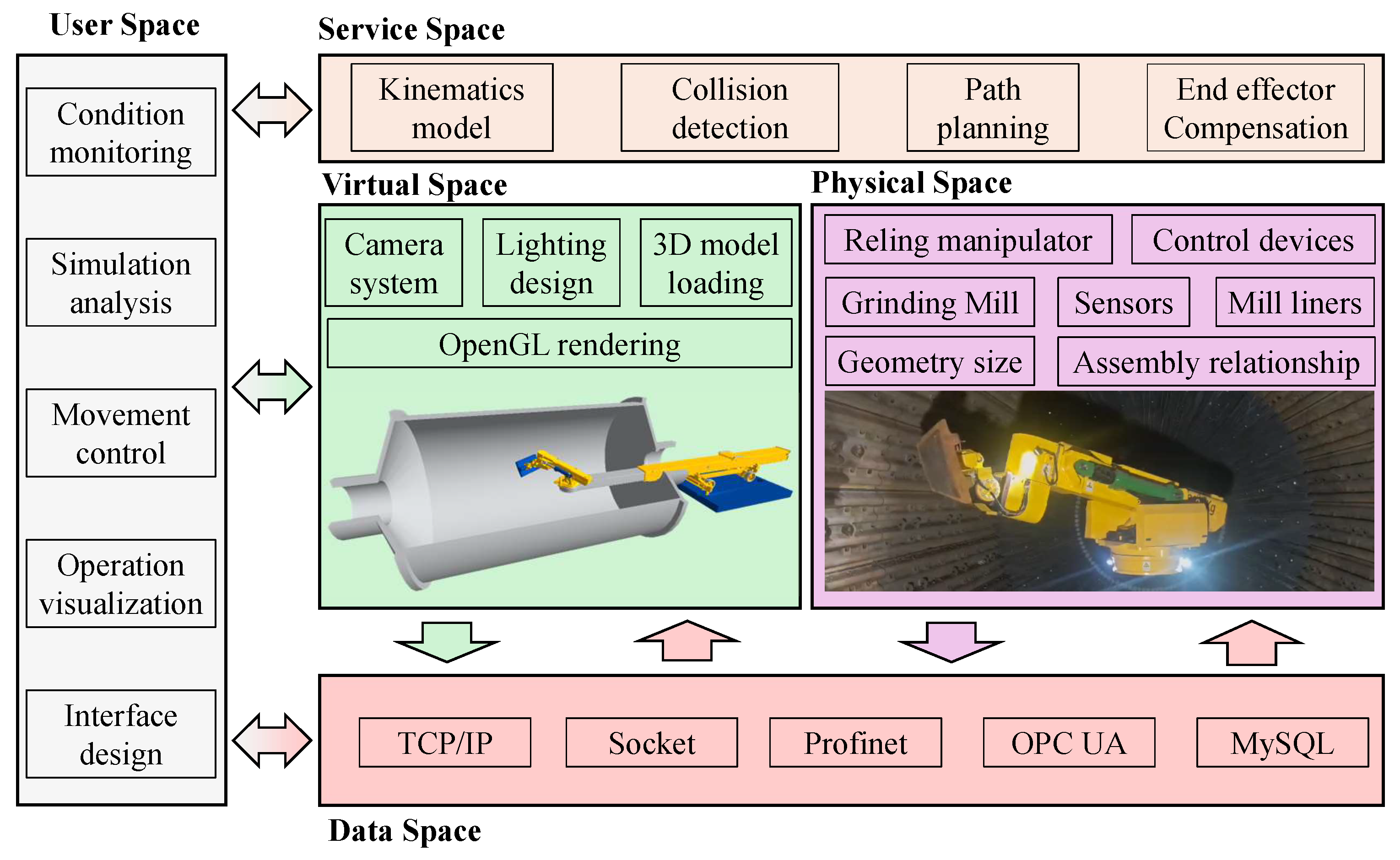
A digital twin aims to establish a real-time mirror model of a real physical scene. In this paper, the process of mill liner exchange is taken as an example to illustrate how to establish the digital twin system step by step for the path planning of a mill relining manipulator. The framework of the established digital twin system is shown in Figure 1; five spaces wewre designed to achieve the real-time mapping between physical space and virtual space. The designed spaces include physical space, virtual space, data space, service space, and user space. Physical space is the foundation of all other spaces. This space not only contains the visible products of the heavy-duty manipulator, mill liners, grinding mill, control devices, and sensors but also consists of the invisible parameters of geometry size, structural characteristics, and assembly relationship. Virtual space is a real-time mapping of the physical space. Based on OpenGL, different modules are designed and integrated for camera control, scene lighting, digital model importation, and manipulator motion in virtual space. Data space is a crucial bridge used to connect the physical entities and virtual space. Based on the TCP/IP protocol, Profinet is used for industrial field data communication, and Socket for remote condition monitoring. OPC UA can be used for data synchronization between the user application and programmable logic controller (PLC). The storage and retrieval of historical data are supported by a MySQL database. Service space provides various functions and algorithms for the virtual space to support the simulation of path planning. Movement analysis, collision detection, path planning, end effector compensation, and safety assessment are conducted in the virtual space before the real operation in the physical scene. The user application was developed for all settings and operations, including condition monitoring, simulation analysis, movement control, and end trajectory and workspace visualization. The established digital twin system can be expressed as follows:

$$\{M,G,C,S,L,O\}\in X$$

(1)

$$\{M^{\prime },G^{\prime },C^{\prime },S^{\prime },L^{\prime },O^{\prime }\}\in P$$

(2)

$$V=F_1(X,P)$$

(3)

$$M=F_2\left(V\right)$$

(4)

where X denotes any physical entities that may appear in the virtual space. $M,G,C,S,L$, and O refer to the 3D digital models of the manipulator, grinding mill, control devices, sensors, liners, and other products, respectively. P represents all useful parameters for the establishment of the digital twin scene. $M^{\prime },G^{\prime },C^{\prime },S^{\prime },L^{\prime }$, and $O^{\prime }$ are the parameters of the corresponding model, such as the geometric information, material properties, location coordinates, and so on. V is the virtual space mapped by the real physical entities. Using X and P as the inputs, the mapping process can be expressed by function $F_1$. Consequently, M can be obtained, which is the virtual model limited by physical constraints, kinematic relationships, and control logic. This is necessary to assure the authenticity of the established digital twin system. The mapping process can be abstractly expressed as function $F_2$.

2.2. Digital Twin Scene Establishment

It is known that many popular established platforms can be used for digital twin establishment, such as Unity, ROS/GAZEBO, MATLAB Robotics Toolbox, and Python-based frameworks. Furthermore, they support the motion simulation of a wide variety of industrial robotic manipulators. However, OpenGL is also introduced in this paper to achieve further customized development and avoid the issues of copyright infringement. The establishment of a digital twin scene mainly includes scene rendering, a camera system, a lighting system, model importation, and joint control. Detailed descriptions are presented in the following sections.

2.2.1. Scene Rendering Based on OpenGL

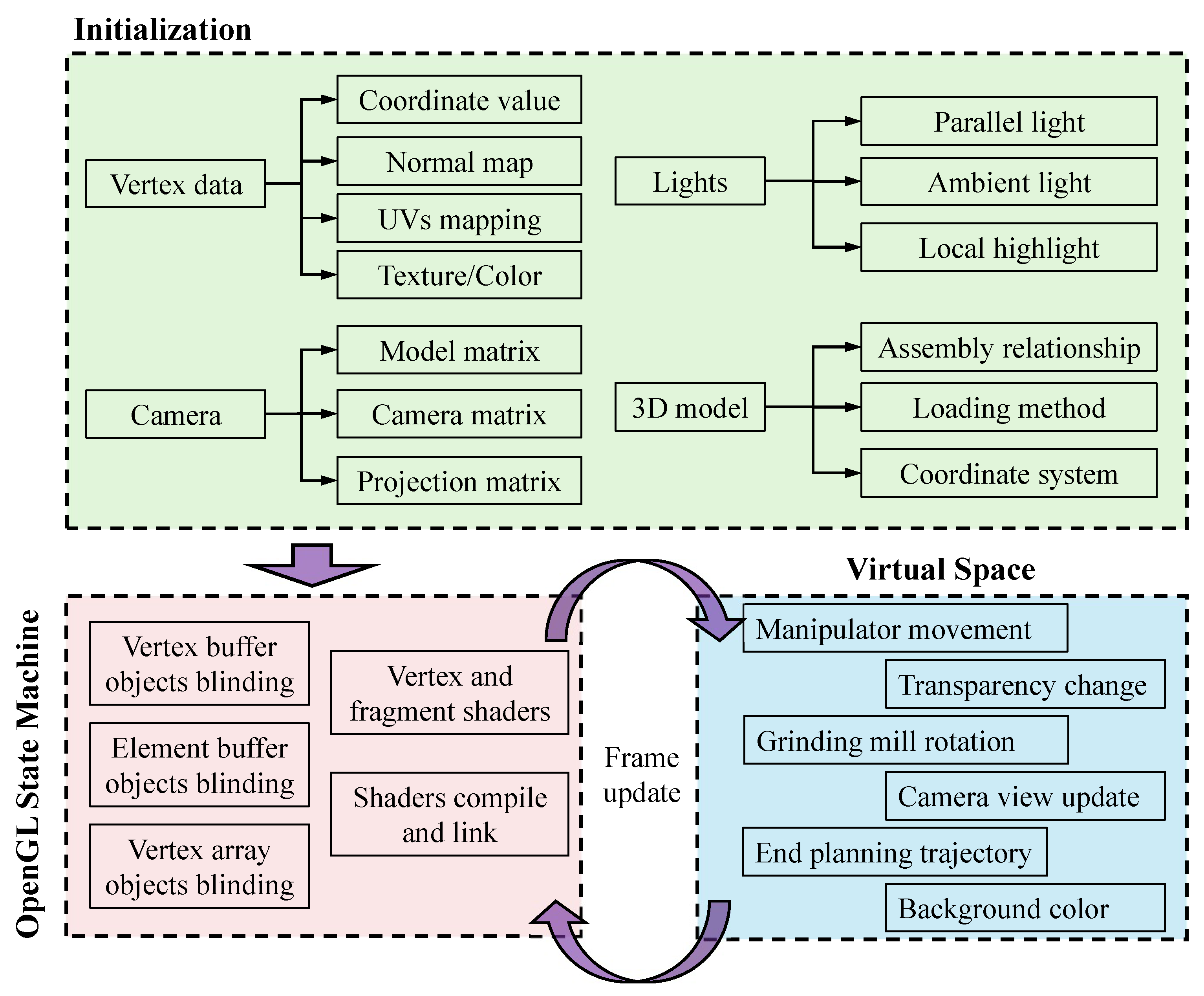
Virtual scene rendering is the foundation of the digital twin system establishment. The function of OpenGL is transforming all 3D coordinates to 2D pixels for display on the screen. As shown in Figure 2, a series of prescribed processes need to be followed. There are three stages that should be implemented for OpenGL programming. First is the initialization stage, and its function is to prepare the necessary parameters for virtual space, such as the triangle unit, camera, lights, and 3D model. The vertex data are the basis for the following scene rendering, and the attributes include coordinate data, normal map, UV mapping, texture, and color. Regarding the camera, lights, and 3D models, detailed explanations are presented in the following sections. OpenGL can be seen as a state machine and its graphics pipeline responsible for managing the transformation of 3D coordinates to 2D pixels. A vertex buffer object (VBO) and element buffer object (EBO) are used to store vertices and indices in the GPU’s memory, respectively. A vertex array object (VAO) stores the configuration of vertex attribute pointers and the bindings of VBOs, allowing OpenGL to know how to fetch vertex data from VBOs during rendering. In programming using OpenGL shading language, vertex and fragment shaders are created, compiled, and linked to calculate the position and the color output of the input pixels. More detailed explanations can be found in the literature [43]. It is widely known that the real industrial scene is changing dynamically, such as manipulator motion, grinding mill rotation, and changes in camera view and object transparency. Therefore, real-time refresh needs to be conducted in virtual space through frame updates to achieve a high-fidelity digital twin model.

2.2.2. Camera System Design

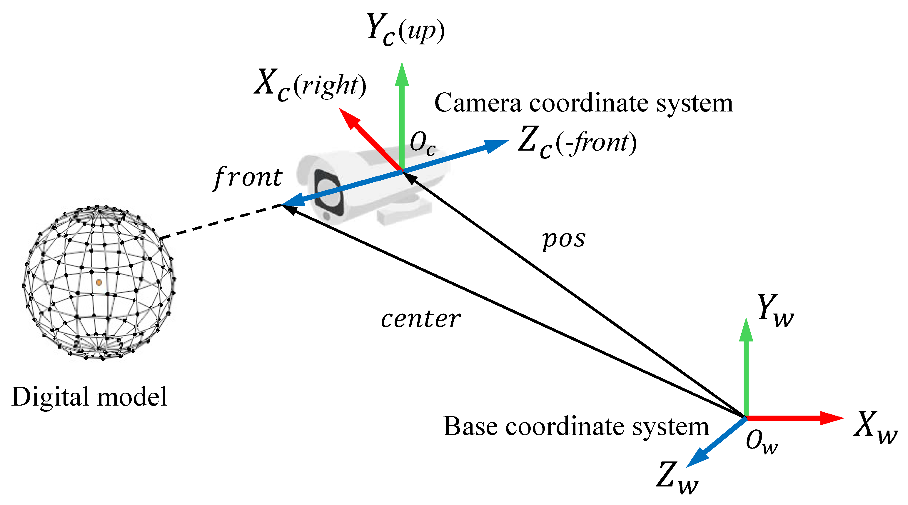
In virtual space, the camera is as crucial as our eyes, enabling us to observe the digital model from different perspectives. The camera system is complex and consists of two main subsystems: the data transformation system and the camera control system. The calculations of the view matrix (VM) and projection matrix (PM) are the main tasks of the data transformation system. As shown in Figure 3, the VM is used to transform all vertex coordinates from global world coordinates $O_w$ to local camera coordinates $O_c$. According to the API provided by OpenGL, the LookAt function can be called to obtain the VM during real-time rendering. It should be noted that three vectors pos, center, and up are necessary for the LookAt function. Here, $pos$ is a known vector and denotes the camera position in $O_w$. The orientation of the camera is represented by the vectors of right, up, and front, which are equal to the known unit vectors x, y, and -z of $O_c$. The direction of the camera is represented by the front vector, which always points to the target object and can be obtained through the cross product of the up and right vectors. Consequently, the VM is ready and waiting to be invoked by the camera system.

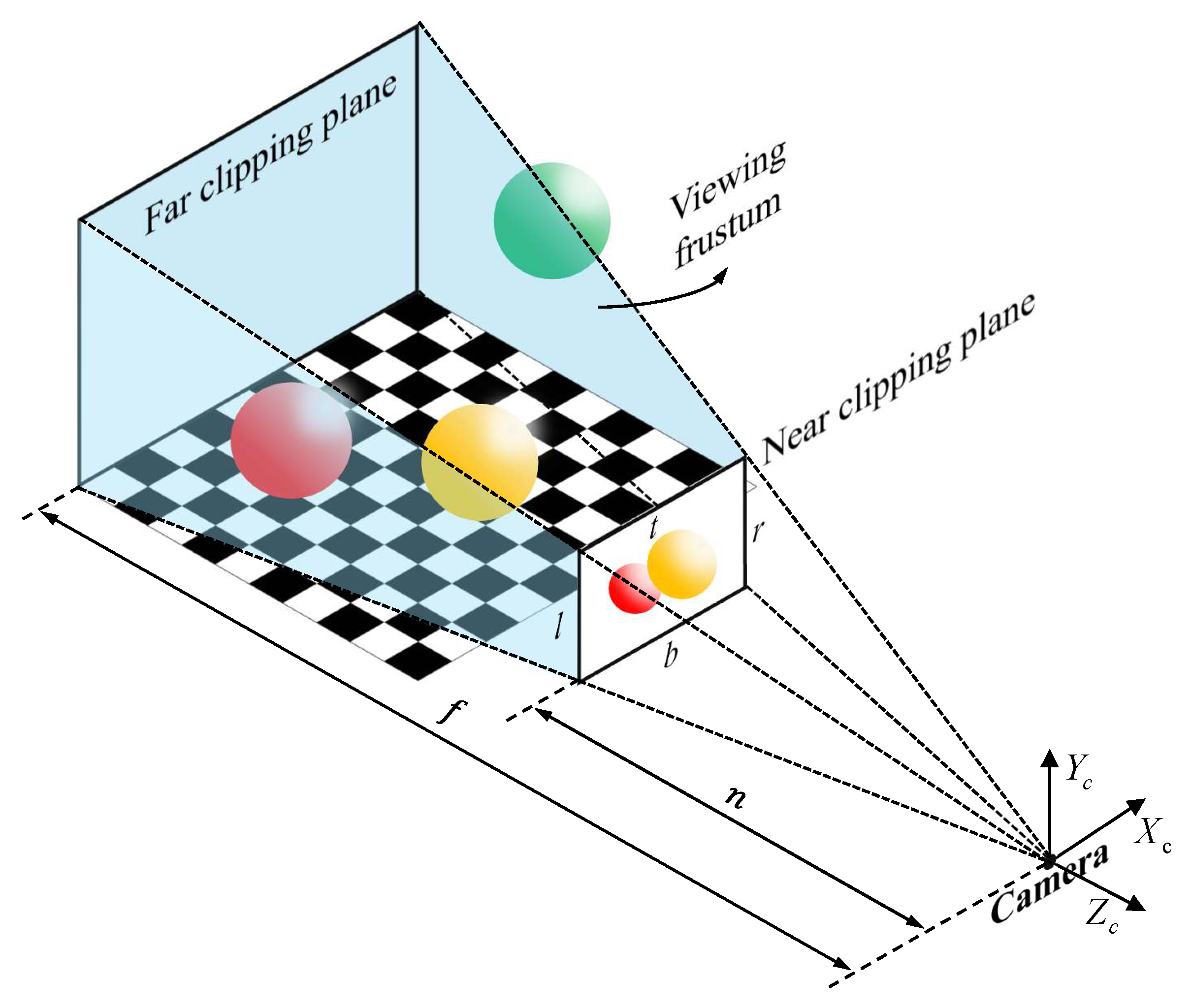
In the world of computer graphics, image projection is generally classified into two types: orthographic projection and perspective projection. In virtual space, perspective projection works similarly to human vision, making objects appear larger at close range and smaller at greater distances. Therefore, PM in this paper refers to the perspective projection matrix. As shown in Figure 4, the space inside of the blue cone is visual space, so-called the viewing frustum (VF), which is decided by the view field of the designed camera, near clipping plane, and far clipping plane. Objects outside the VF cannot be projected to the near clipping plane, as the green ball will be cut off during the graphic pipeline’s processing. As expressed in Equation (5), the PM calculation needs six parameters, including $n,f,l,r,b,$ and t. n and f denote the distances from the camera to the near and far clipping planes, respectively. $l,r,b$, and t represent the coordinates of the left, right, bottom, and top edges of the near clipping plane. Based on the obtained PM, the normalized device coordinate and clip space coordinate are subsequently involved in the OpenGL graphics pipeline. The equation derivation and other detailed explanations are omitted here due to article length limitations. Thus, further details can be found in the literature [43].

$$\mathrm{PM}=\left[\begin{array}{cccc}{\displaystyle \frac{2n}{r-1}}& 0& {\displaystyle \frac{r+l}{r-l}}& 0\\ 0& {\displaystyle \frac{2n}{t-b}}& {\displaystyle \frac{t+b}{t-b}}& 0\\ 0& 0& -{\displaystyle \frac{f+n}{f-n}}& {\displaystyle \frac{-2fn}{f-n}}\\ 0& 0& -1& 0\end{array}\right]$$

(5)

The interactive control of the camera allows us to observe the 3D digital model from different views in virtual space. The main functions include camera rotation, movement, and zoom. As shown in Figure 5, camera control is driven by the operation of mouse cursor movement. By establishing a mapping relationship between the computer cursor and camera’s view matrix, the camera can be controlled accordingly.

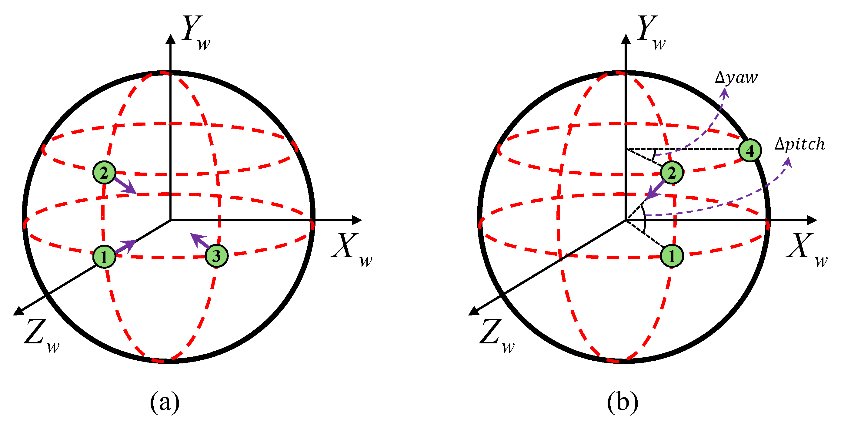
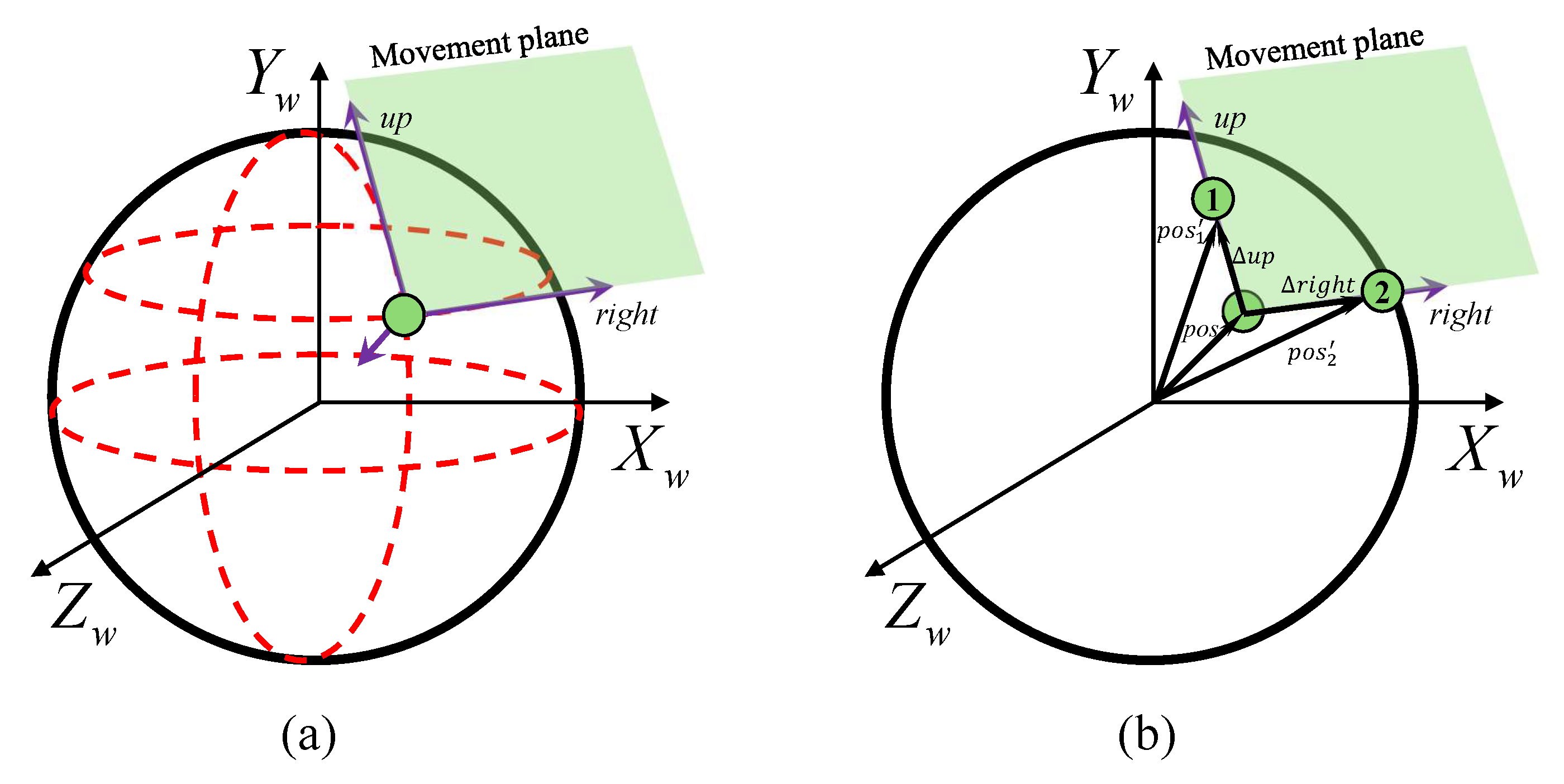
First, the rotation operation involves the camera’s $pos$, $right$, and $up$ vectors. Based on the pixel displacement on the screen, the camera is designed to pitch and yaw according to the mouse movement direction. As indicated in Equation (6), the vertical pixel displacement $\Delta y$ result from cursor movement is used to calculate the new vectors $u{p}^{\prime }$ and $po{s}^{\prime }$. $S_r$ is the rotation adjustment sensitivity. $\mathrm{Rot}(·)$ is the transformation matrix based on Rodrigues’ rotation formula. Likewise, horizontal displacement $\Delta x$ can be used to calculate vectors $u{p}^{\prime }$, $righ{t}^{\prime }$ and $po{s}^{\prime }$, as expressed in Equation (7). The camera rotates around the digital scene in a trackball method; it is locked onto the surface of a sphere, which has a constant radius. As shown in Figure 6a, the camera is designed to move along with the longitude and latitude of the sphere. For instance, if the camera starts at point 1, points 2 and 3 are the results of upward and rightward rotations, respectively. Furthermore, no matter where the camera is located, it always points toward the origin of the sphere. As illustrated in Figure 6b, if the camera starts from point 1 to point 2, the VM should be updated by rotating about the camera’s local axis $X_c$. Regarding the horizontal operation from point 4 to point 2, the rotation axis is the global world axis $Y_w$.

$$[u{p}^{\prime },po{s}^{\prime }]=\mathrm{Rot}(X_c,S_r·\Delta y)\times [up,pos]$$

(6)

$$[u{p}^{\prime },righ{t}^{\prime },po{s}^{\prime }]=\mathrm{Rot}(Y_w,S_r·\Delta x)\times [up,right,pos]$$

(7)

Second, the camera movement enables us to walk around in virtual space. As shown in Figure 7a, movement operation controls the camera to move within a plane defined by the $right$ and $up$ vectors. In this process, unlike with rotation operation, only the camera’s position vector $pos$ needs to be updated according to the movement direction. The mapping relationship is expressed in Equations (8)–(10), where $S_m$ denotes the movement sensitivity, $po{s}^{\prime }$ is the result after mouse operation, and vectors $\Delta right$ and $\Delta up$ denote the displacement along the camera’s right and up direction, respectively. For example, as illustrated in Figure 7b, if the camera’s initial position vector is $pos$, movement along the right direction results in a new position vector $po{s}_2^{\prime }$. Similarly, $po{s}_1^{\prime }$ is the result of upward movement.

$$\Delta right=S_m·\Delta x$$

(8)

$$\Delta up=S_m·\Delta y$$

(9)

$$po{s}^{\prime }=pos+\Delta right+\Delta up$$

(10)

Finally, the principle of camera zoom is straightforward and can be achieved by calculating the new vector $fron{t}^{prime}$, which represents the distance between the camera and the digital object. The zoom operation is determined by the change value $\Delta z$, which is generated by sliding the mouse wheel. The update method is defined by Equation (11), where $\mathrm{Trans}(·)$ is a translation transformation matrix and $-Z_c$ is the target direction. Zoom sensitivity $S_z$ is also introduced to improve operation adjustability.

$$fron{t}^{\prime }=\mathrm{Trans}(-Z_c,S_z·\Delta z)\times front$$

(11)

Figure 7. Camera movement control based on trackball method. (a) Definition of the camera movement plane; (b) Examples of camera movement in different directions.

Figure 7. Camera movement control based on trackball method. (a) Definition of the camera movement plane; (b) Examples of camera movement in different directions.

2.2.3. Light System Design

In the real world, without lights, nothing can be seen. This sentence emphasizes the importance of lights in virtual space. In the computer world, lighting effects can be simulated through different lighting models. The Phong lighting model was employed due to its computational simplicity, which simulates lighting effects through the color interaction between a light source and object surfaces. It is well known that color information is stored in memory in the form of RGB’s three channels. In virtual space, everything can be seen as an object with different RGB values. The difference is that the RGB value represents the lighting intensity for the light source. However, for rendered objects, the RGB values denote the color reflection intensity, which differs from the material properties. The designed system incorporates four types of lighting effects: directional light simulating sunlight, diffuse and specular reflection from object surfaces, and ambient light resulting from indirect illumination by surrounding objects. Figure 8 presents the generation process of diffuse light and specular highlights based on the interaction between directional light and virtual objects. It can be seen that a little directional light is absorbed by the object itself, as indicated by the gray arrows. The remainder is redistributed into the surrounding environment through diffuse and specular reflection components, represented by the yellow arrows. Unlike with the diffuse light, the highlight has a higher lighting strength and is symmetrical to incident light. Regarding ambient light, a constant ambient vector is given to multiple object color vectors to simulate the overall brightness of the virtual scene. Finally, taking four lights into account together, a comprehensive lighting system can be established for the digital twin system.

2.2.4. Model Importation and Joint Control

Usually, complex mechanical equipment is designed using third-party professional 3D CAD software, such as CATIA, UG, SolidWorks, or Croe. With these tools, workers can improve the efficiency of 3D model development, but it also raises the following problem: how is this external model imported into virtual space without losing the assembly relationship at the same time? Therefore, to address the above problems, the Open Asset Import Library (Assimp) is used to import the prepared 3D models in FBX format. A recursive approach is conducted to extract all relevant model attributes, such as mesh structures, position coordinates, textures, materials, and hierarchical relationships. After 3D model importing, the corresponding link system should be designed to support the manipulator joint control in the virtual digital scene. As shown in Figure 9, the entire system consists of eight control joints: two prismatic joints, five rotation joints, and one virtual joint. These joints are connected sequentially to form parent–child link pairs. All control joints share the same coordinate orientation with base 0 coordinate, where the green axis denotes the rotation or movement axis depending on the joint type. Specifically, joints 1 is designed for the upper arm control, and it is responsible for the forward and backward movement of the entire manipulator. Rotation joints 2 and 3 are designed to control the forearm’s swivel and pitch. Similarly for the upper arm, joint 4 in charge of the forearm movement. Regarding the wrist component, rotation joints 5, 6, and 7 provide more flexibility for mill liner grasping tasks, while virtual joint 8 is used to visualize the position and orientation of the end effector. To ensure the fidelity of the digital twin model, it is important to emphasize that the control joints designed in this section are consistent with the kinematic coordinate system introduced in the following section. After the establishment of the digital twin scene, the physical entities should be connected through sensor data collection and real-time communication.

2.3. Sensor Data Collection and Transmission

Data collection and transmission are essential to ensure the authenticity of the digital twin system, including static structural data and dynamic operation data. Static structural data include geometric dimensions, physical properties, spatial position, and assembly relationships. The above-mentioned data can be obtained through instrument-based measurements and serve as the basis for digital modeling and virtual space establishment. Dynamic operation data mainly include real-time sensor data, operation instructions, and other feedback data. As shown in

Table 1. Sensor parameters for different monitor objects.

Monitor Objects	Range Ability	Sensor Type	Precision	Number
Upper arm movement	0∼6000 mm	Drawstring displacement	0.25% F.S.	2
Forearm swing	0∼360°	Grating angle encoder	$\pm {0.5}^{″}$	1
Forearm pitch	$\pm \mathrm{50°}$	Uniaxial inclination	0.25% F.S.	1
Forearm movement	0∼2500 mm	Drawstring displacement	0.25% F.S.	2
Wrist swing	$\pm \mathrm{60°}$	Grating angle encoder	$\pm 1^{″}$	1
Wrist pitch	$-\mathrm{105°}$∼30°	Grating angle encoder	$\pm {2.5}^{″}$	1
Wrist roll	$\pm \mathrm{50°}$	Grating angle encoder	$\pm {2.5}^{″}$	1
End effector operation	0∼500 mm	Drawstring displacement	0.25% F.S.	2

F.S. denotes full scale of measurement range.

, the grating angle encoder is used to monitor forearm rotation, wrist swing, wrist roll, and wrist pitch. The drawstring displacement sensor is not only used for the end effector grasping but it is also responsible for measuring the movements of the upper arm and the forearm. In addition, a uniaxial inclination sensor is utilized to capture the rotation angle during forearm pitch. Except the sensor data collection, bidirectional data transmission should be established to support path planning simulation in the digital twin system. In this paper, the grinding mill equipment, mill relining manipulator, and associated control devices are connected to the host computer through the Profinet bus to ensure real-time data communication. A Siemens S7-1200 PLC (manufactured in Munich, Germany) was used to control the manipulator. The acquired data include the launch signal, joint angles, movement speed, and other control data. Between virtual space and PLC, OPC UA and Socket communication technologies are introduced for the realization of virtual–real mapping. The detailed steps are as follows.

From physical entities to virtual space: (1) based on TIA Portal V16 and PLC S7-1200, an OPC UA server was built to store the control variables; (2) communication between OPC UA and Socket was established to enable data transmission; (3) the received data was processed within virtual space and the digital model of the mill relining manipulator was updated.

From virtual space to physical entities: (1) based on the path planning simulation, the improved joint configuration sequence is obtained; (2) according to the received data, the corresponding control data in the OPC UA server are updated; (3) PLC controls the physical manipulator to complete mill liner exchange task.

3. Path Planning and End Effector Compensation

In practical engineering applications, manipulator movement simulation should be implemented in the virtual space first to verify the safety and accuracy of mill liner exchange. Therefore, based on the established digital twin scene, this section focuses on the path planning algorithm and end effector compensation strategy. Furthermore, a geometry-based collision detection method is also proposed to support the path planning task.

3.1. Mill Liner Exchange Process

The function of mill liners is to protect the mill shell from the aggressive environment inside the grinding mill. They are installed inside of the grinding mill and distributed around the inner surface. Therefore, the mill relining manipulator is operated inside the grinding mill. Figure 10 shows the process of liner installation. Under the starting configuration, the manipulator needs to grasp the liner from the transport trailer in a back-looking configuration. Figure 10b shows the goal configuration for installing a sidewall liner. The task of mill liner exchange is to determine a suitable path from the start configuration to the goal configuration. At the same time, end effector deformation should be considered to ensure mounting hole alignment. The manipulator should coordinate all joints to accomplish the liner installation task. During motion, the liner is attached to the end effector, and they have the same posture.

3.2. Manipulator Kinematics Model

As shown in Figure 11, the heavy-duty equipment is a seven-DOF redundant manipulator and consists of five rotational joints and two prismatic joints. During operation, it is necessary to control both the position and orientation of the end effector to complete the liner installation.

Table 2. Joint effects on position and orientation of end effector.

	${\mathit{q}}_1$	${\mathit{q}}_2$	${\mathit{q}}_3$	${\mathit{q}}_4$	${\mathit{q}}_5$	${\mathit{q}}_6$	${\mathit{q}}_7$
Position	◯	◯	◯	◯	◯	◯	⨂
Orientation	⨂	◯	◯	⨂	◯	◯	◯

◯ indicates that the joint affects the position or orientation; ⨂ denotes no effect.

shows the effects of each joint to the end effector, where q represents the generalized joint. Joints $q_2$, $q_3$, $q_5$, and $q_6$ affect not only the position but also the orientation. Prismatic joints $q_1$ and $q_4$ only affect the position, and joint $q_7$ only affects the orientation adjustment.

Based on the right-hand rule, the Modified Denavit–Hartenberg (MD-H) method [44] is used to establish the base coordinate system and other joint coordinate systems. The red, green, and blue arrows represent the axes of x, y, and z, respectively. Therefore, the forward kinematics model can be obtained, which is a foundation for the following path planning scheme. MD-H parameters are shown in

Table 3. MD-H parameters of mill relining manipulator.

Link i	1	2	3	4	5	6	7
${\alpha }_{i-1}$ (rad)	0	$-\pi /2$	$-\pi /2$	$\pi /2$	$-\pi /2$	$\pi /2$	$\pi /2$
$a_{i-1}$ (mm)	0	0	40	559	0	280	70
${\theta }_i$ (rad)	0	${\theta }_2$	${\theta }_3$	$-\pi /2$	${\theta }_5$	${\theta }_6$	${\theta }_7$
$d_i$ (mm)	$d_1$	230.5	0	$d_4$	−741	0	0

. ${\alpha }_{i-1}$, $a_{i-1}$, $d_i$, and ${\theta }_i$ represent the twist angle, link length, link offset, and joint angle, respectively. $d_1$, $d_4$, ${\theta }_2$, ${\theta }_3$, ${\theta }_5$, ${\theta }_6$, and ${\theta }_7$ are the actuated variables that drive the motion of the manipulator. The general transformation matrix between adjacent joint coordinate frames $i-1$ and i is given by Equation (12), where $\mathrm{Rot}(·)$ and $\mathrm{Trans}(·)$ represent the rotation transformation matrix and translation transformation matrix, respectively.

Table 4. Constraints of rotation and prismatic joints.

	${\mathit{q}}_1$ (mm)	${\mathit{q}}_2$ (°)	${\mathit{q}}_3$ (°)	${\mathit{q}}_4$ (mm)	${\mathit{q}}_5$ (°)	${\mathit{q}}_6$ (°)	${\mathit{q}}_7$ (°)
$q_i^{min}$	0	−180	−35	0	−75	−105	−180
$q_i^{max}$	11,500	180	40	3000	75	30	180

shows the constraints of the rotation and prismatic joints.

$$\begin{array}{c}{}_{\mathit{i\hspace{1em} }}{}^{i-1}T=\mathrm{Rot}(X,{\alpha }_{i-1})\mathrm{Trans}(X,a_{i-1})\mathrm{Rot}(Z,{\theta }_i)\mathrm{Trans}(Z,d_i)=\hfill \\ \left[\begin{array}{cccc}cos{\theta }_i& -sin{\theta }_i& 0& a_{i-1}\\ sin{\theta }_{i}cos{\alpha }_{i-1}& cos{\theta }_{i}cos{\alpha }_{i-1}& -sin{\alpha }_{i-1}& -sin{\alpha }_{i-1}{d}_i\\ sin{\theta }_{i}sin{\alpha }_{i-1}& cos{\theta }_{i}sin{\alpha }_{i-1}& cos{\alpha }_{i-1}& cos{\alpha }_{i-1}{d}_i\\ 0& 0& 0& 1\end{array}\right]\hfill \end{array}$$

(12)

Finally, the forward kinematics model of the manipulator can be derived through successive matrix multiplication, as expressed in Equation (13). $\mathbf{R}=[\mathbf{n},\mathbf{o},\mathbf{a}]$ represents the orientation of the end effector, where $\mathbf{n}=[n_x,n_y,n_z]$, $\mathbf{o}=[o_x,o_y,o_z]$, and $\mathbf{a}=[a_x,a_y,a_z]$ are the unit direction vectors of the x, y, and z axes in coordinate system $O_7$, respectively. $\mathbf{P}=[p_x,p_y,p_z]$ is the position vector of $O_7$ relative to the base coordinate system $O_0$. Solving the forward kinematics involves calculating the transformation matrix ${}_7{}^{0}T$ based on the known joint configuration.

$${}_7{}^{0}T={}_1{}^{0}T{}_2{}^{1}T{}_3{}^{2}T{}_4{}^{3}T{}_5{}^{4}T{}_6{}^{5}T{}_7{}^{6}T=\left[\begin{array}{cccc}{n}_x& o_x& a_x& p_x\\ n_y& o_y& a_y& p_y\\ n_z& o_z& a_z& p_z\\ 0& 0& 0& 1\end{array}\right]=\left[\begin{array}{cc}\mathbf{R}& \mathbf{P}\\ 0& 1\end{array}\right]$$

(13)

3.3. Collision Detection

To ensure safety during path planning, collision detection is necessary and should be conducted in the virtual space before operating real physical manipulator. Based on the inside geometric structure of the grinding mill, an effective collision detection method is proposed in this paper. As shown in Figure 12, the closer the manipulator is to the red mill center axis and the farther it is from the mill wall, the safer it is. Based on the vertex coordinate, the distance between key check points and the mill wall can be used as a collision judgment criterium. Therefore, the signed distance field (SDF) is introduced to reflect safe credibility. The mill is symmetrical and can be separated into three parts: a middle large cylinder, cones at both ends, and two small cylinders as an inlet or outlet for the manipulator. Therefore, based on the idea of segmentation calculation, the SDF distribution heatmap is established. From the results, it can be seen that a closer red dotted axis indicates a greater distance from the mill inside surface. 

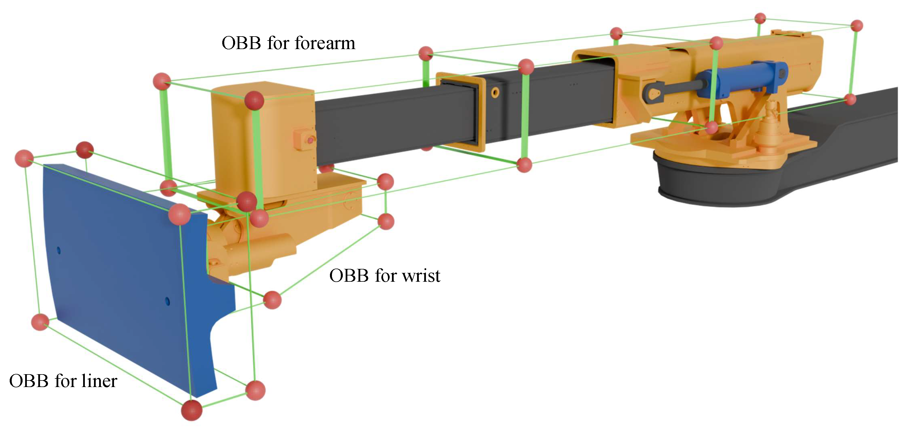
Despite the above distance calculation method, the crucial check points of the mill relining manipulator should be designed for collision detection implementation. The oriented bounding box (OBB) is a common method used in a lot of collision detection experiments [45]. Furthermore, the mill relining manipulator is a structured redundant robotic arms. As shown in Figure 13, OBB is also introduced to limit the boundary of the manipulator. Through geometric and motion analysis of manipulator, the upper arm is a prismatic joint that remains parallel to the mill axis, ensuring that no collision occurs during movement. Therefore, it is sufficient to apply OBB to the manipulator’s forearm, wrist, and liner. In consideration of the joints’ dynamic adjustment during movement, the check points in OBB are designed to adaptively change in response to the joint configuration change.

3.4. Path Planning Algorithm

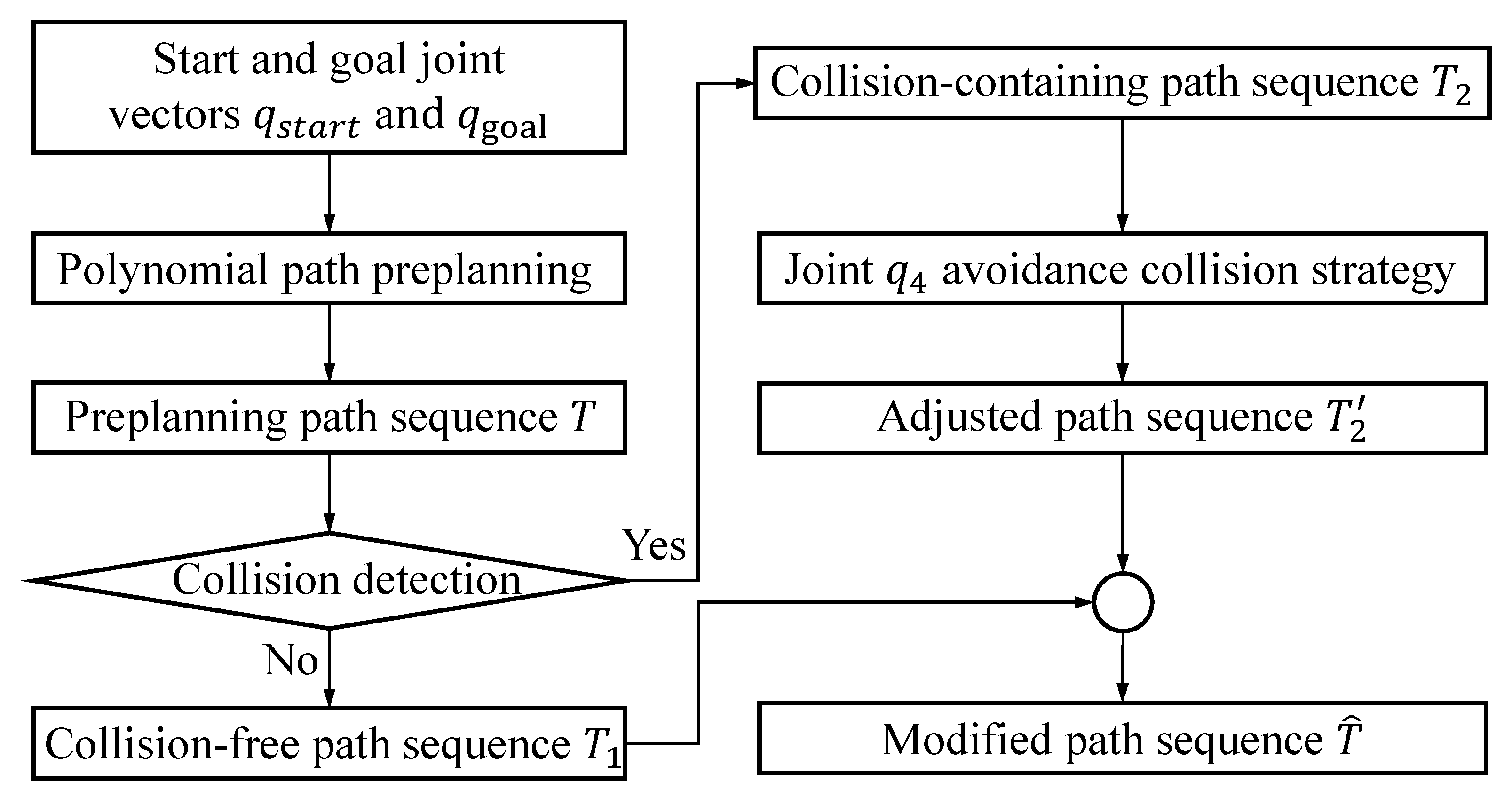
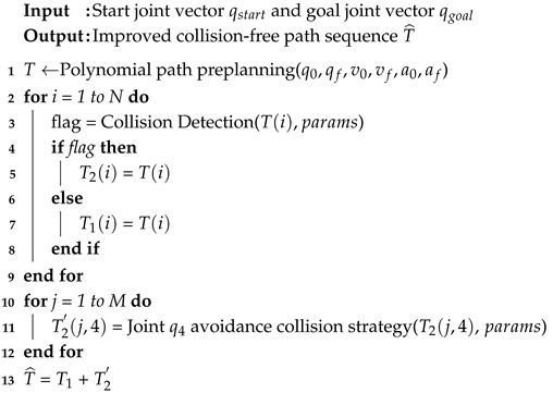
The path planning algorithm is implemented in joint space, and the flowchart is shown in Figure 14. The proposed path planning method includes two stages: path preplanning and avoidance collision adjustment. According to the geometic structure of the grinding mill, it should be emphasized that all collisions can be avoided by reducing the prismatic joint $q_4$. A detailed explanation is presented as follows. 

First, the start joint vector $q_{start}$ is predefined according to the position of the liner transport trailer. The goal joint vector $q_{goal}$ is given according to the inverse kinematics solution of the target installation position. Second, path preplanning is carried out by the fifth-order polynomial function [46]. The boundary constraints are mainly applied at the start and end of the path planning, including the starting position $q_0$ and ending position $q_f$, velocities $v_0$ and $v_f$, and accelerations $a_0$ and $a_f$. Consequently, the preplanning path sequence $T\in {\mathbb{R}}^{N\times 7}$ can be obtained. N represents the number of discrete planning steps of the path motion, and 7 is the number of joint degrees of freedom in the redundant mill reline manipulator. However, collision detection is not involved in this stage; T consists of collision-free path sequence $T_1\in {\mathbb{R}}^{(N-M)\times 7}$ and collision-containing path sequence $T_2\in {\mathbb{R}}^{M\times 7}$, that is, $T=T_1+T_2$. Third, the avoidance collision strategies are proposed for joint $q_4$ to obtain adjusted path sequence $T_2^{\prime }$, and a detailed explanation will be presented below. Finally, the modified path sequence $\widehat{T}=T_1+T_2^{\prime }$ can be obtained, which not only performs well in liner relining tasks but is also collision-free with respect to the inside surface of the grinding mill. The pseudocode of the proposed path planning algorithm is shown in Algorithm 1. The input and output are $[q_{start},q_{goal}]$, and the collision-free path sequence is $\widehat{T}$. $params$ denotes the structure parameters, including the mill’s geometric data, the collision check points, and forward kinematics model.

Based on the analysis of the manipulator motion, prismatic joint $q_1$ is excluded from the collision detection since it always moves along the central axis of the mill. Additionally, there is no optimal space for joints $q_2$ and $q_3$, which are heavily restricted by the target joint configuration. Wrist joints $q_5$, $q_6$, and $q_7$ have a small impact on collision avoidance. Therefore, the proposed collision-avoiding strategies are focused on joint $q_4$. Furthermore, two working scenarios need to be considered: the middle cylinder area and the conical area.

Algorithm 1: Pseudocode of the proposed path planning algorithm

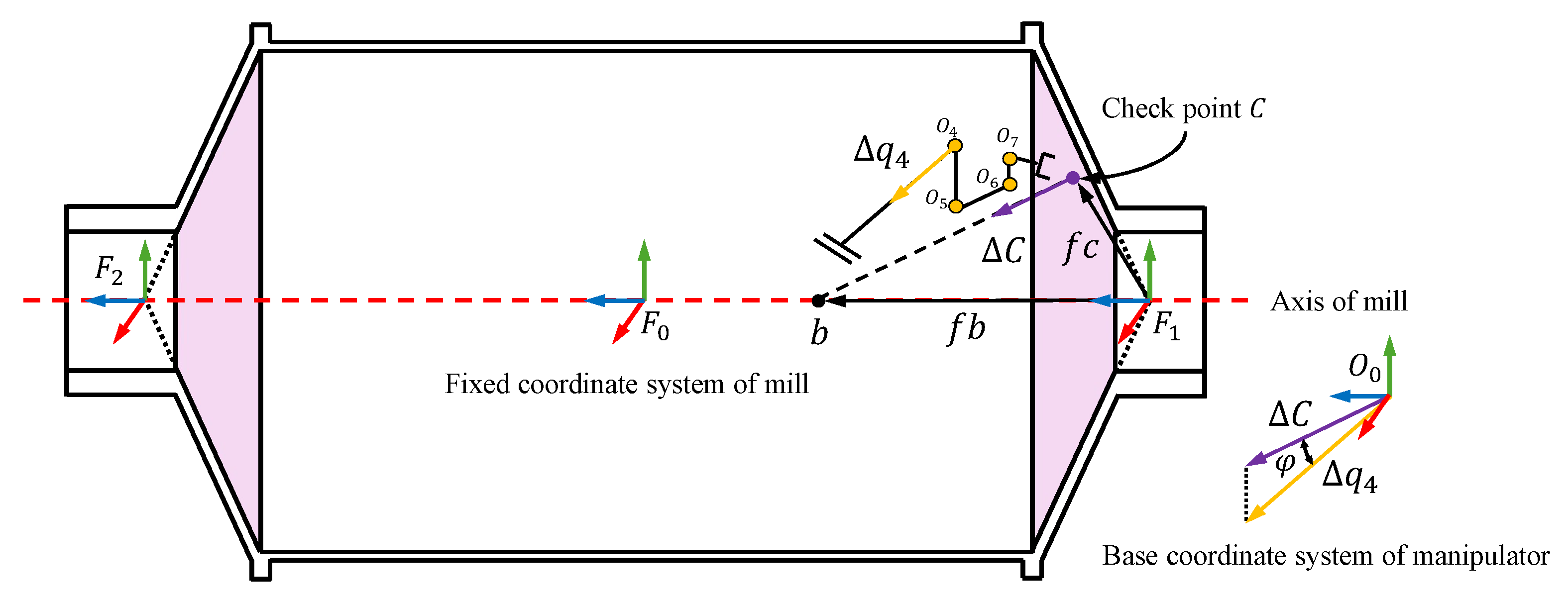
In the cylinder area, the collision avoidance strategy for joint $q_4$ is shown in Figure 15, where joints $q_1$, $q_2$, and $q_3$ are not shown for simplicity. The proposed strategy is an analytical method that not only prevents collisions but also avoids unnecessary movement. Among all check points of the manipulator, we assume that the purple check point C is the closest point to the inner wall. Through the proposed SDF collision method, $D_c$ is the distance between C and the inside surface of the grinding mill. In the current situation, $D_c$ does not satisfy the required safety distance threshold $D_s$. Therefore, check point C has to move away from the inner wall and closer to the red axis of the mill. The manipulator should move a distance of $|\Delta C|$ in the direction of vector $\Delta C$. Furthermore, vector $\Delta C$ is perpendicular to the z-axis of $F_0$ (or the red axis of the mill). During online detection, $|\Delta C|$ can be calculated through the difference between $D_c$ and $D_s$. As expressed in Equation (14), the analytical collision-free adjustment value $\Delta q_4$ can be derived from $\Delta C$. Here, $\phi$ is the angle between vector $\Delta C$ and the unit z-axis vector ${\widehat{z}}_4$ of joint $q_4$ at this moment. The direction of $\Delta C$ is the same as $(x_{F_0}^c,y_{F_0}^c,0)$, which is the projection of C onto the x-y plane in the $F_0$ coordinate system. It is important to note that all calculations need to be conducted in the base coordinate system $O_0$, as illustrated in the bottom right corner.

$$\Delta q_4={\displaystyle \frac{\left|\Delta C\right|}{cos\phi }}={\displaystyle \frac{D_c-D_s}{cos\phi }}$$

(14)

$$\phi =arccos(\Delta C·{\widehat{z}}_4/\left|\Delta C\right|·\left|{\widehat{z}}_4\right|)$$

(15)

In the conical area, the additional fixed coordinate systems, ${\mathrm{F}}_1$ and ${\mathrm{F}}_2$, need to be established at the vertices of the cones, respectively. Their axes are also aligned with the fixed coordinate system ${\mathrm{F}}_0$. Unlike with the cylinder area, the main challenge is solving the direction of $\Delta C$, and the proposed collision avoidance strategy in the near conical area is shown in Figure 16. In the fixed coordinate system ${\mathrm{F}}_1$, the position of check point C can be defined as vector $fc=(x_{F_1}^c,y_{F_1}^c,z_{F_1}^c)$. Point b is assumed to be located on the central axis of the mill or the z-axis of ${\mathrm{F}}_1$, so position vector $fb$ is $(0,0,z_{F_1}^b)$. On this basis, $(fb-fc)$ can be calculated, and the result is $(-x_{F_1}^c,-y_{F_1}^c,z_{F_1}^b-z_{F_1}^c)$, and $\Delta C$ has the same direction as this vector. Although $(x_{F_1}^c,y_{F_1}^c,z_{F_1}^c)$ can be obtained through forward kinematics, $z_{F_1}^b$ is unknown. In the current situation, check point C is very close to the inner surface of the mill, and $fc$ and $\Delta C$ can be assumed to be approximately perpendicular with each other. On this basis, $z_{F_1}^b$ can be obtained using $fc·(fb-fc)=0$, and the function is expressed in Equation (16). Consequently, the fastest direction away from the conical surface can be calculated indirectly as ${\displaystyle \frac{\Delta C}{|\Delta C|}}={\displaystyle \frac{(fb-fc)}{\left(\right|fb-fc\left|\right)}}$. Additionally, the values of $\phi$, $D_c$, $D_s$, and $\Delta q_4$ are the same as the check points in the cylinder area, as expressed in Equations (14) and (15). The calculation for the far conical area should be conducted in ${\mathrm{F}}_2$, and the principle is similar.

$$z_{F_1}^b={\displaystyle \frac{{\left(x_{F_1}^c\right)}^2+{\left(y_{F_1}^c\right)}^2+{\left(z_{F_1}^c\right)}^2}{z_{F_1}^c}}$$

(16)

3.5. Online End Effector Compensation Strategy

It should be noted that the above obtained theoretical path cannot be directly applied to the physical manipulator. The reason for this is the inherent characteristics of the mill relining manipulator: large structural mass, high end payload, and long action distance. Under the effect of gravity, centimeter-level deformation exists at the end effector. Therefore, an online end effector compensation method is proposed to improve motion reliability and liner installation accuracy. The details are explained as follows:

(1)

According to the constraints of each joint, a lot of discrete joint configuration combinations are selected to comprehensively reflect the working conditions in the joint space.

(2)

The FE static models are established for each joint configuration.

(3)

All FE models are solved, recording the corresponding end effector deformation to form an offline deformation dataset. As illustrated in Figure 17, the end effector deformations cover the entire workspace. Furthermore, the end deformation increases with the distance from the base frame.

(4)

Based on the offline dataset and fitting algorithm, an online calculation algorithm is proposed for real-time end deformation prediction.

(5)

With the guidance of the above compensation data, a modified motion path can be obtained through appropriate joint adjustment.

Figure 17. Cloud map of end effector deformation based on FE simulation.

Figure 17. Cloud map of end effector deformation based on FE simulation.

It should be noted that the focus of this paper is to realize the fast online deformation calculation in a digital twin system based on the established offline database, rather than developing a best fitting algorithm. Utilizing the obtained end deformation samples as a training dataset, a BP neural network [47] is employed to fit the nonlinear relationship between joint configurations and end effector deformation, so that we can demonstrate the feasibility and effectiveness of fast online prediction. The designed neural network has four input neurons (corresponding to joints $q_1$, $q_2$, $q_3$, and $q_4$), one output neuron (end effector deformation), and ten hidden layers. The training steps of the neural network are as follows:

(1)

Joint configuration normalization. Due to the dimensions of the rotation and prismatic joints being different, the normalization should be conducted before model training, and the calculation is expressed in Equation (17). $q_i^{\min }$ and $q_i^{\max }$ denote the minimum and maximum values of the ith joint, respectively. This min-max normalization scales the input data to the range [0, 1], thereby enhancing the stability and convergence performance of the model during training.

$$q_i^{\mathrm{norm}}={\displaystyle \frac{q_i-q_i^{min}}{q_i^{max}-q_i^{min}}}$$

(17)

(2)

Forward neural network. In the neural network, input data are processed through multiple nonlinear transformations across hidden layers, and the output of each layer is shown in Equation (18). Here, l denotes the index of the network layer, i and j are the indexes of the neuron. $z_i^l$ is the pre-activation value of the ith neuron in layer l. $W_{ij}^{(l-1)}$ is the weight that connects the jth neuron in layer $l-1$ to the ith neuron in layer l. $a_j^{(l-1)}$ represents the output of the jth neuron in layer $l-1$. $b_i^l$ is the bias term associated with the ith neuron in layer l. $a_i^l$ is the output after activation function $f(·)$, which can provide the capability of nonlinear fitting.

$$z_i^l=\sum _{j=1}^{s_l}{W}_{ij}^{(l-1)}{a}_j^{(l-1)}+b_i^l$$

(18)

$$a_i^l=f\left(z_i^l\right)$$

(19)

(3)

Cost function calculation. End deformation prediction is a regression problem. Therefore, the mean squared error (MSE) is employed as the cost function to quantify the discrepancy between the ith predicted output ${\widehat{y}}_i$ and the ground truth label $y_i$. $J(W,b)$ is the objective function, and the input parameters are the trainable weights W and biases b of the network. n is the number of training examples.

$$J(W,b)={\displaystyle \frac{1}{n}}\sum _{i=1}^n{({\widehat{y}}_i(W,b)-y_i)}^2$$

(20)

(4)

Error backpropagation. To update the network model, the partial derivatives of $J(W,b)$ with respect to the weight and bias are calculated. The gradient descent and learning rate $\alpha$ are employed to iteratively adjust network parameters. The process is as follows:

$$W_{ij}^{\left(l\right)}\leftarrow W_{ij}^{\left(l\right)}-\alpha {\displaystyle \frac{\partial J(W,b)}{\partial W_{ij}^{\left(l\right)}}}$$

(21)

$$b_i^{\left(l\right)}\leftarrow b_i^{\left(l\right)}-\alpha {\displaystyle \frac{\partial J(W,b)}{\partial b_i^{\left(l\right)}}}$$

(22)

Subsequently, we repeat steps (2) to (4) to update the weights and biases until the MSE is below the predefined tolerance or the maximum number of iterations is reached. The end deformation prediction model M enables real-time calculation, as in Equation (23). $\widehat{U}$ is the predicted deformation, and vector Q denotes the input joint configuration vector.

$$\widehat{U}=M\left(Q\right)$$

(23)

4. Application Development and Path Planning Simulation

4.1. User Interface Design and Function Description

In this study, a user desktop application was developed for the manipulator’s real-time condition monitoring. Based on .Net Framework, C# programming language, and OpenTK and AssimpNet toolkits, the designed user interface is illustrated in Figure 18. Multiple modules are integrated into the main interface, including digital model rendering in the central panel, motion control for joints $q_1-q_7$ in the top-left area, workspace visualization in the bottom-left area, joint change curves in the bottom panel, and the end effector posture matrix in the bottom-right area. Additionally, rendering settings, background color, component visibility, and camera views can be directly adjusted via buttons, checkboxes, and trackbars. In this system, the improved path sequence can be obtained through simulation analysis in virtual space. Furthermore, the collision detection, path planning algorithm, and online end effector compensation method are integrated into this software. With the designed desktop application, the digital twin system not only reflects the condition of the physical manipulator but also enables its real-time operation.

Furthermore, the workspace visualization function was also designed in this application, which allows us to observe the manipulator’s working range in an intuitive way. As shown in Figure 19, based on forward kinematics and the Monte Carlo method, 50,000 discrete sample points are generated by solving different random joint configurations. Each green sphere represents the corresponding end effector position. Figure 19a–c shows the distribution of all reachable points from different views. From the side view and top view, it can be found that the manipulator can fully cover the internal space of the grinding mill in all directions. Through sample distribution analysis, the density of the near-base frame and mill bottom areas is higher than others, indicating that the manipulator exhibits greater flexibility in these areas. The diversity and high solvability result in a higher probability of sample generation. Therefore, the manipulator is prone to operate in a swing posture with a downward pitch. Furthermore, the rotation of the mill is performed in cooperation with the manipulator motion.

4.2. Case Study for Path Planning Algorithm

To further verify the superiority of the proposed path planning algorithm, comparison experiments were conducted in this study. Three popular planning algorithms were involved in the following experiments, and the details are discussed as follows:

(1)

Based on a bidirectional rapidly-exploring random tree [21], the improved Bi-RRT algorithm for the mill reline manipulator (Bi-RRT-M) is used for comparison in this experiment. Bi-RRT-M is also a kind of sampling-based method and has a double-tree structure. This makes it achieve higher efficiency and lower time costs in the search process. To adapt this algorithm to the redundant mill reline manipulator, the solution dimensions are set to 7, and the joint update step is shown in Table 5. The random sampling probability and maximum number of iterations are set to 0.5 and 2000, respectively. When the distance between the current and desired end effector positions falls below 50 mm, the iteration loop terminates, and the planning results are recorded.

(2)

Based on the original APF algorithm [23], the improved APF for the mill reline manipulator (APF-M) is used as the second comparison algorithm. The attractive force is generated by the target joint vector, while the direction of the repulsive force is the same as the decreasing direction of joint $q_4$. The coefficients of the attractive and repulsive forces are set to 1000 and 0.001, respectively. The repulsive force influence radius is set to 4000 mm. The update step size and termination condition are the same as those used in the Bi-RRT-M. Moreover, hard constraints are imposed on the joints throughout path planning.

(3)

The fast analytical path planning algorithm (FAPP) is the algorithm proposed in this paper, which is an analytical-based algorithm that reduces joint $q_4$ to avoid collision during manipulator motion.

Table 5. Joint update step size for Bi-RRT-M algorithm.

Joints	${\mathit{q}}_1$ (mm)	${\mathit{q}}_2$ (°)	${\mathit{q}}_3$ (°)	${\mathit{q}}_4$ (mm)	${\mathit{q}}_5$ (°)	${\mathit{q}}_6$ (°)	${\mathit{q}}_7$ (°)
Step	100	1.0	1.0	100	1.0	1.0	1.0

Table 5. Joint update step size for Bi-RRT-M algorithm.

Joints	${\mathit{q}}_1$ (mm)	${\mathit{q}}_2$ (°)	${\mathit{q}}_3$ (°)	${\mathit{q}}_4$ (mm)	${\mathit{q}}_5$ (°)	${\mathit{q}}_6$ (°)	${\mathit{q}}_7$ (°)
Step	100	1.0	1.0	100	1.0	1.0	1.0

The case study in this paper involves exchanging a far-cone-area liner with a simulation method using the established digital twin system. This path planning task is difficult, since joint $q_2$ has to bypass the middle cylinder area through significant rotation. During motion, the confined space increases the challenge of collision avoidance. In addition, a solution is not easy to achieve due to the long motion distance. In this experiment, the input parameters include start and goal joint configurations, as shown in

Table 6. Joint configurations of the start and goal positions for liner exchange in the far cone area.

Joints	${\mathit{q}}_1$ (mm)	${\mathit{q}}_2$ (°)	${\mathit{q}}_3$ (°)	${\mathit{q}}_4$ (mm)	${\mathit{q}}_5$ (°)	${\mathit{q}}_6$ (°)	${\mathit{q}}_7$ (°)
Start	8100	−180	15	2000	0	−103	0
Goal	9747.7	−15.0	−5.8	3000	−6.8	−6.5	−151.7

. Consequently, the output of each algorithm is a collision-free path sequence for manipulator motion. The evaluation metrics include planning time to assess computational efficiency, path length to indicate energy consumption, and the number of path nodes to reflect the planning complexity. The experimental results of different algorithms are presented in

Table 7. Path planning results of different algorithms for mill liner exchange.

Algorithms	Planning Time (s)	Path Length (mm)	Path Nodes
Bi-RRT-M	17.83	21,683.9	129
APF-M	3.08	17,209.7	329
FAPP	1.70	15,299.0	100

, where the performance of the proposed method is outstanding in all evaluation metrics. FAPP only needs 1.70 s to finish the collision-free path planning, and it is approximately 10.5 times faster than Bi-RRT-M. In a confined environment, sampling-based methods are not suitable for enabling the manipulator to quickly avoid the inner wall around it, because it acts like a huge obstacle. Although the planning time of the APF-M algorithm is 3.08s, which has a significant improvement in planning speed, the number of path nodes increases since there are no greedy characteristics. Compared with the common algorithm, the path lengths of FAPP are 15,299 mm. This outstanding performance demonstrates that the proposed framework is effective and efficient.

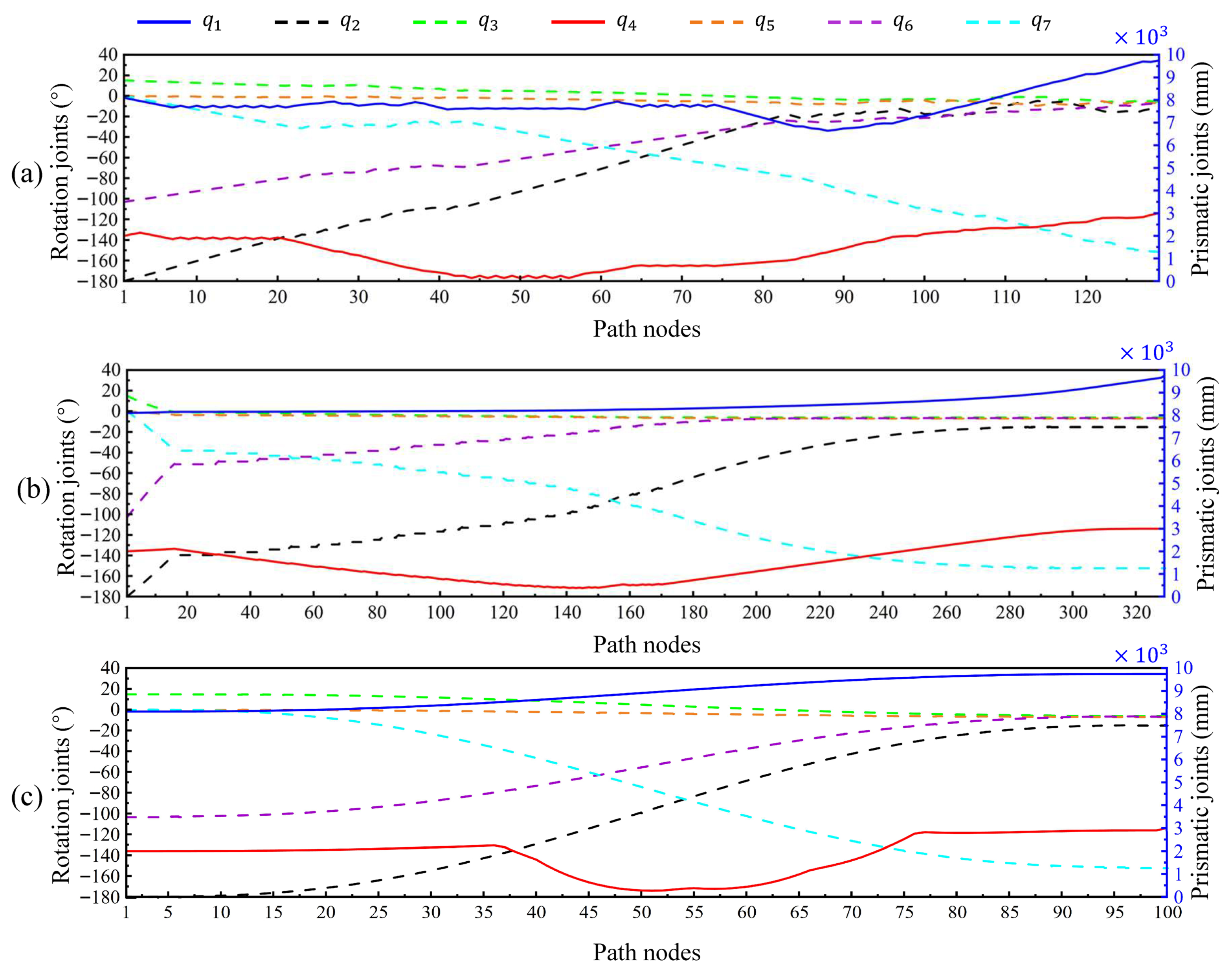
As shown in Figure 20, we also visualize the motion trajectories of different algorithms; it can be observed that the smoothest trajectory is the proposed FAPP. Due to the influence of random sampling, the trajectory of Bi-RRT-M exhibits significant irregularities, with oscillations and reverse motion tendencies in some local paths, which are unacceptable for controlling a heavy-duty manipulator. As for the path trajectory of the APF-M algorithm, there are many noticeable oscillations in the corner at the starting stage. The reason for this is the non-adaptive update step and the interaction between the repulsive force from the inner wall and the attractive force from the goal joint vector. Figure 20c shows the end trajectory of FAPP, and the motion process is presented in Figure 20d–h, where the motion is smooth and continuous. Figure 21 shows the curves of different algorithms for far-cone liner relining in joint space, where the labels of the x-axis represent the path planning nodes. Figure 21a–c show the trend curves generated by Bi-RRT-M, APF-M, and FAPP, respectively. Based on the above analysis, the joints of Bi-RRT-M changes occur in most path nodes, leading to low stability during motion. However, FAPP achieves the smoothest curve in not only the prismatic joint $q_4$ but also the other joints.

4.3. End Effector Compensation Simulation

Based on the planned path, the end effector carrying the mill liner is expected to follow the desired trajectory to the target position. However, due to the influence of gravity, the actual end trajectory inevitably deviates from the theoretical path, which decreases end positioning accuracy and increases the risk of collision. As shown in Figure 22a, the gray solid line indicates the desired end trajectory, whereas the green discrete spheres are the deviated actual end trajectories. As the manipulator extends, the distance between the end effector and the fixed frame increases, leading to deformation increases, especially at the installation position, where the end deformation reaches the maximum. Therefore, the proposed online end deformation calculation method is used in this section to minimize end deviation through the digital twin system.

The obtained theoretical path sequence $Q\in {\mathbb{R}}^{n\times 7}$ consists of n path node vectors $q\in {\mathbb{R}}^{1\times 7}$, and each row represents a single joint configuration. During the end compensation process, every joint configuration needs to be modified, involving the proposed path planning algorithm, online end deformation prediction, and forward and inverse kinematics. The specific steps are outlined as follows:

(1)

Obtain theoretical path sequence Q based on the proposed path planning method.

(2)

Obtain the ith joint configuration vector $q_i$ and the corresponding end effector transformation matrix $T_i$ based on forward kinematics.

(3)

Calculate the end effector deformation $u_i$ according to the obtained joint configuration $q_i$.

(4)

Modify $T_i$ based on the above $u_i$ and obtain compensated transformation matrix $T_i^{\prime }$.

(5)

Solve $T_i^{\prime }$ through inverse kinematics to obtain modified joint configuration vector $q_i^{\prime }$.

(6)

Repeat steps 2–5 to obtain each modified $q_i^{\prime }$ and form modified path sequence $Q^{\prime }$.

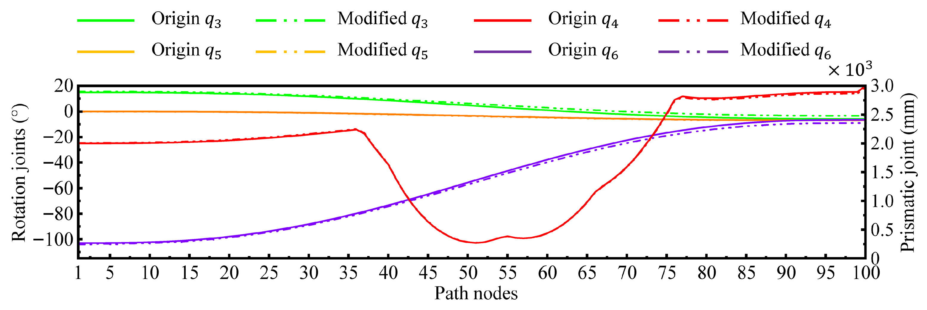
Figure 23 illustrates the difference between the original and modified change curves of joints $q_3$, $q_4$, $q_5$, and $q_6$, while joints $q_1$ and $q_2$ are not presented because they do not contribute to the end compensation process. It can be found that joint $q_3$ plays a critical role in end compensation, owing to its pitch adjustment capability. Joints $q_4$ and $q_6$ are involved in adjusting the posture changes in the manipulator caused by the change in $q_3$. Since joint $q_5$ is in charge of the wrist’s swing, it has little effect on end compensation. Detailed comparison results between the original and modified joint values are available in the Supplementary Materials.

The position tracking error of the end effector, defined as the difference between the desired and actual trajectories, is also analyzed in this section and presented in Figure 24. In the world base coordinate system, the position errors along the X, Y, and Z-axes are shown in Figure 24a–c, respectively. Figure 24d presents the absolute position error. It is not difficult to find that the main error is from the Y-axis, caused by the effects of gravity. By comparing the $q_4$ curve in Figure 23 with the absolute tracking error in Figure 24d, it can be observed that the error trend correlates with the extension of the manipulator. From path nodes 40 to 53, joint $q_4$ decreases and the end position error also decreases. From path node 40 to 53, a decrease is observed in the end tracking error, which coincides with a reduction in joint $q_4$. In contrast, from path nodes 58 to 78, an increase in both joint $q_4$ and the tracking error is observed. Furthermore, the errors in all directions are within 2 mm, meeting the accuracy requirements for mill liner exchange during mounting hole alignment.

A visualization of the modified end trajectory is also presented in Figure 22b. Although slight deviations exist at some local path nodes, the actual trajectory is nearly coincident with the desired trajectory. Through the motion simulation within the digital twin system, the manipulator can accurately follow the desired trajectory. Furthermore, collisions can be effectively avoided, and the accuracy of end positioning is enhanced even under complex working conditions.

5. Conclusions

This paper not only establishes a digital twin system but also proposes a path planning algorithm and end effector compensation method for the mill relining manipulator. First, a digital twin framework is proposed, comprising five interconnected spaces responsible for physical entity control, virtual model simulation, service function drivers, bidirectional data transmission, and user space interaction. Consequently, based on OpenGL, the scene rendering, camera system, light designs, digital model importation, and joint controls are explained to establish a comprehensive digital twin system. The sensor data collection and transmission method are also discussed to support the virtual–real interaction. Second, based on the kinematics model and collision detection, a path planning algorithm is proposed to simulate the mill liner exchange task within the digital twin system. In addition, an online end effector deformation calculation method is proposed to reduce the end trajectory tracking error caused by gravity effects. Finally, a user desktop application is developed based on the above-mentioned methods to realize mill relining manipulator real-time condition monitoring and simulation analysis visualization. Furthermore, comparison experiments were conducted on path planning to demonstrate the superiority of the proposed algorithm in terms of planning speed, path length, and motion smoothness. Not limited to the theoretical path, an end effector deformation simulation experiment is presented to demonstrate the effectiveness of the proposed online compensation method. The joint path sequence is improved, and the end effector absolute tracking error is satisfied for practical application.

However, there are also some limitations of this study. For instance, due to article length limitations, further technical discussion and algorithmic insight for each method is not presented in this paper. In addition, since the prototype platform is still under development, the effectiveness of the proposed digital twin system cannot be demonstrated through hardware experiments at this time. In the future, we will continue to explore mill relining manipulator control strategies and prototype development works. The effectiveness of the proposed digital twin system and path planning algorithm will be further verified on the hardware platform.

References

1. Cabral, J.V.A.; Álvares, A.J.; Guilherme, C.d.C. Digital twin implementation for an additive manufacturing robotic cell based on the iso 23247 standard. IEEE Latin Am. Trans. 2024, 22, 651–658. [Google Scholar] [CrossRef]
2. Angelidis, G.; Bampis, L. Gesture-controlled robotic arm for small assembly lines. Machines 2025, 13, 182. [Google Scholar] [CrossRef]
3. Ma, S.; Deng, K.; Lu, Y.; Xu, X. Robot error compensation based on incremental extreme learning machines and an improved sparrow search algorithm. Int. J. Adv. Manuf. Technol. 2023, 125, 5431–5443. [Google Scholar] [CrossRef]
4. Cai, J.; Lei, T. An autonomous positioning method of tube-to-tubesheet welding robot based on coordinate transformation and template matching. IEEE Robot. Autom. Lett. 2021, 6, 787–794. [Google Scholar] [CrossRef]
5. Gu, J.; He, S.; Dai, J.; Wei, D.; Yan, H.; Tan, C.; Wang, Z.; Si, L. A walking trajectory tracking control based on uncertainties estimation for a drilling robot for rockburst prevention. Machines 2024, 12, 298. [Google Scholar] [CrossRef]
6. Zhang, X.; Huang, M.; Lei, M.; Tian, H.; Chen, X.; Tian, C. Improved rapid-expanding-random-tree-based trajectory planning on drill arm of anchor drilling robots. Machines 2023, 11, 858. [Google Scholar] [CrossRef]
7. Zhang, J.; Wang, Y.; Che, L.; Wang, N.; Bai, Y.; Wang, C. Workspace analysis and motion control strategy of robotic mine anchor drilling truck manipulator based on the WOA-FOPID algorithm. Front. Earth Sci. 2022, 10, 954547. [Google Scholar] [CrossRef]
8. Liu, Y.; Yi, W.; Feng, Z.; Yao, J.; Zhao, Y. Design and motion planning of a 7-DOF assembly robot with heavy load in spacecraft module. Robot. Comput.-Integr. Manuf. 2024, 86, 102645. [Google Scholar] [CrossRef]
9. Dong, D.; Wang, Z.; Guan, J.; Xiao, Y.; Wang, Y. Research on key technology and application progress of rescue robot in nuclear accident emergency situation. Nucl. Eng. Technol. 2025, 57, 103457. [Google Scholar] [CrossRef]
10. Wang, Q.; Wu, H.; Song, Y.; Handroos, H.; Cheng, Y.; Qin, G. Parameter identification of heavy-duty manipulator using stochastic gradient Hamilton Monte Carlo method. IEEE Access 2023, 11, 78561–78583. [Google Scholar] [CrossRef]
11. Yahyaei, M.; Powell, M.; Toor, P.; Tuxford, A.; Limpus, A. Relining efficiency and liner design for improved plant performance. Miner. Eng. 2015, 83, 64–77. [Google Scholar] [CrossRef]
12. Rao, J.; Xiang, C.; Xi, J.; Chen, J.; Lei, J.; Giernacki, W.; Liu, M. Path planning for dual UAVs cooperative suspension transport based on artificial potential field-A* algorithm. Knowl.-Based Syst. 2023, 277, 110797. [Google Scholar] [CrossRef]
13. Rückin, J.; Magistri, F.; Stachniss, C.; Popović, M. An Informative Path Planning Framework for Active Learning in UAV-Based Semantic Mapping. IEEE Trans. Robot. 2023, 39, 4279–4296. [Google Scholar] [CrossRef]
14. Pour Arab, D.; Spisser, M.; Essert, C. 3D hybrid path planning for optimized coverage of agricultural fields: A novel approach for wheeled robots. J. Field Robot. 2025, 42, 455–473. [Google Scholar] [CrossRef]
15. Pi, Y.; Liu, X.; Yang, Z.; Zhong, Y.; Huang, T.; Pu, H.; Luo, J. OMEPP: Online Multi-Population Evolutionary Path Planning for Mobile Manipulators in Dynamic Environments. IEEE Trans. Autom. Sci. Eng. 2024, 22, 6234–6245. [Google Scholar] [CrossRef]
16. Dijkstra, E.W. A note on two problems in connexion with graphs. Numer. Math. 1959, 1, 269–271. [Google Scholar] [CrossRef]
17. Hart, P.E.; Nilsson, N.J.; Raphael, B. A formal basis for the heuristic determination of minimum cost paths. IEEE Trans. Syst. Sci. Cybern. 1968, 4, 100–107. [Google Scholar] [CrossRef]
18. Stentz, A. Optimal and efficient path planning for partially-known environments. In Proceedings of the the 1994 IEEE International Conference on Robotics and Automation, San Diego, CA, USA, 8 May 1994; IEEE: Piscataway, NJ, USA, 1994; pp. 3310–3317. [Google Scholar] [CrossRef]
19. Karaman, S.; Frazzoli, E. Sampling-based algorithms for optimal motion planning. Int. J. Robot. Res. 2011, 30, 846–894. [Google Scholar] [CrossRef]
20. LaValle, S.M. Rapidly-Exploring Random Trees: A New Tool for Path Planning; Technical Report 98-11; Computer Science Department, Iowa State University: Ames, IA, USA, 1998. [Google Scholar]
21. Kuffner, J.J.; LaValle, S.M. RRT-connect: An efficient approach to single-query path planning. In Proceedings of the 2000 ICRA, Millennium Conference, IEEE International Conference on Robotics and Automation, Symposia Proceedings (Cat. No. 00CH37065), San Francisco, CA, USA, 24–28 April 2000; IEEE: Piscataway, NJ, USA, 2000; Volume 2, pp. 995–1001. [Google Scholar]
22. Gammell, J.D.; Srinivasa, S.S.; Barfoot, T.D. Informed RRT*: Optimal sampling-based path planning focused via direct sampling of an admissible ellipsoidal heuristic. In Proceedings of the 2014 IEEE/RSJ International Conference on Intelligent Robots and Systems, Chicago, IL, USA, 14–18 September 2014; IEEE: Piscataway, NJ, USA, 2014; pp. 2997–3004. [Google Scholar]
23. Tian, Y.; Zhu, X.; Meng, D.; Wang, X.; Liang, B. An overall configuration planning method of continuum hyper-redundant manipulators based on improved artificial potential field method. IEEE Robot. Autom. Lett. 2021, 6, 4867–4874. [Google Scholar] [CrossRef]
24. Jiang, Q.; Cai, K.; Xu, F. Obstacle-avoidance path planning based on the improved artificial potential field for a 5 degrees of freedom bending robot. Mech. Sci. 2023, 14, 87–97. [Google Scholar] [CrossRef]
25. Zhou, C.; Wang, Y.; Li, R.; Guan, T.; Liu, Z.; Peng, G.; You, K. Artificial intelligence technology for path planning of automated earthwork machinery. J. Field Robot. 2024, 42, 1887–1913. [Google Scholar] [CrossRef]
26. Grieves, M.W. Product lifecycle management: The new paradigm for enterprises. Int. J. Prod. Dev. 2005, 2, 71–84. [Google Scholar] [CrossRef]
27. Zhang, L.; Liu, J.; Zhuang, C. Digital twin modeling enabled machine tool intelligence: A review. Chin. J. Mech. Eng. 2024, 37, 47. [Google Scholar] [CrossRef]
28. Thoben, K.D.; Wiesner, S.; Wuest, T. “Industrie 4.0” and smart manufacturing-a review of research issues and application examples. Int. J. Automot. Technol. 2017, 11, 4–16. [Google Scholar] [CrossRef]
29. Liu, Y.; Xu, H.; Liu, D.; Wang, L. A digital twin-based sim-to-real transfer for deep reinforcement learning-enabled industrial robot grasping. Robot. Comput.-Integr. Manuf. 2022, 78, 102365. [Google Scholar] [CrossRef]
30. Liu, W.; Zou, X.; Wen, Z.; Cheng, J.; Zuo, Y.; Zhang, C.; Liu, H.; Tao, F. Digital twin-based production-logistics synchronization system for satellite mass assembly shop-floor. Chin. J. Mech. Eng. 2024, 37, 163. [Google Scholar] [CrossRef]
31. Singh, M.; Kapukotuwa, J.; Gouveia, E.L.S.; Fuenmayor, E.; Qiao, Y.; Murry, N.; Devine, D. Unity and ROS as a digital and communication layer for digital twin application: Case study of robotic arm in a smart manufacturing cell. Sensors 2024, 24, 5680. [Google Scholar] [CrossRef]
32. Lai, X.; Wang, S.; Guo, Z.; Zhang, C.; Sun, W.; Song, X. Designing a shape–performance integrated digital twin based on multiple models and dynamic data: A boom crane example. J. Mech. Des. 2021, 143, 071703. [Google Scholar] [CrossRef]
33. Duan, J.; Gong, X.; Zhang, Q.; Qin, J. A digital twin–driven monitoring framework for dual-robot collaborative manipulation. Int. J. Adv. Manuf. Technol. 2023, 125, 4579–4599. [Google Scholar] [CrossRef]
34. Farhadi, A.; Lee, S.K.; Hinchy, E.P.; O’Dowd, N.P.; McCarthy, C.T. The development of a digital twin framework for an industrial robotic drilling process. Sensors 2022, 22, 7232. [Google Scholar] [CrossRef]
35. Guo, X.; Peng, G.; Meng, Y. A modified Q-learning algorithm for robot path planning in a digital twin assembly system. Int. J. Adv. Manuf. Technol. 2022, 119, 3951–3961. [Google Scholar] [CrossRef]
36. Hou, M.; Cao, H.; Shi, J.; Guo, Y. An industry-oriented digital twin model for predicting posture-dependent FRFs of industrial robots. Mech. Syst. Signal Proc. 2024, 212, 111251. [Google Scholar] [CrossRef]
37. Garg, G.; Kuts, V.; Anbarjafari, G. Digital twin for FANUC robots: Industrial robot programming and simulation using virtual reality. Sustainability 2021, 13, 10336. [Google Scholar] [CrossRef]
38. Liu, X.; Jiang, D.; Tao, B.; Jiang, G.; Sun, Y.; Kong, J.; Tong, X.; Zhao, G.; Chen, B. Genetic algorithm-based trajectory optimization for digital twin robots. Front. Bioeng. Biotechnol. 2022, 9, 793782. [Google Scholar] [CrossRef]
39. Wang, W.; Ding, W.; Hua, C.; Zhang, H.; Feng, H.; Yao, Y. A digital twin for 3D path planning of large-span curved-arm gantry robot. Robot. Comput.-Integr. Manuf. 2022, 76, 102330. [Google Scholar] [CrossRef]
40. Zuo, C.; Cheng, Y.; Pan, H.; Qin, G.; Zhou, P.; Xia, L.; Wang, H.; Zhao, R.; Lv, Y.; Qin, X.; et al. Research on accurate morphology predictive control of CFETR multi-purpose overload robot. Nucl. Eng. Technol. 2024, 56, 4412–4422. [Google Scholar] [CrossRef]
41. Xiong, G.; Ye, L.; Zhang, X.; Gao, Y.; Hua, Z.; Dapeng, Y.; Yu, C.; Tang, Q. Multipoint variable parameter compliant control of redundant manipulator based on the equivalent twin model of flexible contact dynamics. Int. J. Adv. Robot. Syst. 2024, 21, 1–16. [Google Scholar] [CrossRef]
42. Liu, S.; Cheng, Y.; Lu, K.; Qin, G.; Pan, H.; Zuo, C. Development of a digital twin system for snake endoscope manipulator in fusion reactors. Nucl. Eng. Technol. 2025, 57, 103283. [Google Scholar] [CrossRef]
43. Hughes, J.F.; van Dam, A.; McGuire, M.; Sklar, D.F.; Foley, J.D.; Feiner, S.K.; Akeley, K. Computer Graphics: Principles and Practice, 3rd ed.; Addison-Wesley: Upper Saddle River, NJ, USA, 2014; pp. 455–466. [Google Scholar]
44. Sung, M.; Choi, Y. Algorithmic modified denavit–hartenberg modeling for robotic manipulators using line geometry. Appl. Sci. 2025, 15, 4999. [Google Scholar] [CrossRef]
45. Chang, J.W.; Wang, W.; Kim, M.S. Efficient collision detection using a dual OBB-sphere bounding volume hierarchy. Comput.-Aided Des. 2010, 42, 50–57. [Google Scholar] [CrossRef]
46. Singh, G.; Banga, V.K. Combinations of novel hybrid optimization algorithms-based trajectory planning analysis for an industrial robotic manipulators. J. Field Robot. 2022, 39, 650–674. [Google Scholar] [CrossRef]
47. Ding, S.; Su, C.; Yu, J. An optimizing BP neural network algorithm based on genetic algorithm. Artif. Intell. Rev. 2011, 36, 153–162. [Google Scholar] [CrossRef]
Figure 1. Digital twin system framework for mill liner exchange scene.
Machines 13 00823 g001
Figure 2. Virtual scene rendering and frame update based on OpenGL.
Machines 13 00823 g002
Figure 3. View matrix calculation based on transformation relationship between global world and local camera coordinates.
Machines 13 00823 g003
Figure 4. Principles and parameters of perspective projection. The red and yellow balls represent the objects within the viewing frustum. Green ball does not appear on the near clipping plane, as it lies outside the viewing frustum.
Machines 13 00823 g004
Figure 5. Update flow chart of camera control.
Machines 13 00823 g005
Figure 6. Camera rotation control based on trackball method. Point 1 is the initial position of camera. Points 2, 3 and 4 show the results after rotation operation. (a) Different camera postures on the trackball surface; (b) Explanation of different camera rotation directions.
Machines 13 00823 g006
Figure 8. Interaction between light and rendering objects. (a) Diffuse reflection light; (b) specular reflection highlight.
Machines 13 00823 g008
Figure 9. Designed control joints of mill relining manipulator.
Machines 13 00823 g009
Figure 10. Liner installation process using mill relining manipulator. The blue object represents the carried liner, the yellow indicates the mill relining manipulator, and the grinding mill is shown in gray. (a) Axonometric view of start configuration; (b) axonometric view of goal configuration.
Machines 13 00823 g010
Figure 11. Mill relining equipment and MD-H coordinate systems.
Machines 13 00823 g011
Figure 12. Heatmap of the signed distance field distribution inside the grinding mill. The red dotted line represents the central axis of the grinding mill.
Machines 13 00823 g012
Figure 13. Oriented bounding boxes and sparse check points for collision detection.
Machines 13 00823 g013
Figure 14. Flowchart of proposed path planning algorithm.
Machines 13 00823 g014
Figure 15. Collision avoidance strategy in cylinder area for joint q 4 .
Machines 13 00823 g015
Figure 16. Collision avoidance strategy in conical area for joint q 4 .
Machines 13 00823 g016
Figure 18. User desktop application for mill relining manipulator digital twin system.
Machines 13 00823 g018
Figure 19. Workspace visualization of mill relining manipulator. (a) Axonometric view; (b) side view; (c) top view.
Machines 13 00823 g019
Figure 20. Path planning visualization of different algorithms for mill liner exchange. (a) Bi-RRT-M; (b) APF-M; (c) the proposed FAPP; (dh) enclosed by the dashed box and illustrate the different steps of FAPP.
Machines 13 00823 g020
Figure 21. Curves of different algorithms for far-cone liner exchange in joint space. (a) Bi-RRT-M; (b) APF-M; (c) the proposed FAPP.
Machines 13 00823 g021
Figure 22. Motion simulation and result comparison between desired and actual end trajectories. Gray solid line and green discrete spheres represent the desired and actual end motion trajectories, respectively. (a) Without end effector deformation compensation; (b) with end effector deformation compensation.
Machines 13 00823 g022
Figure 23. Original and modified change curves of joints q 3 , q 4 , q 5 , and q 6 .
Machines 13 00823 g023
Figure 24. Position errors of end effector after deformation compensation. (a) Position error of X-axis; (b) position error of Y-axis; (c) position error of Z-axis; (d) absolute position error.
Machines 13 00823 g024