An Optimized Active Compensation Control Framework for High-Speed Railway Pantograph via Imitation-Guided Deep Reinforcement Learning

Abstract

Extreme pantograph–catenary contact force (PCCF) oscillations pose a serious challenge to the stable coupling between pantograph and catenary in high-speed railway systems. This paper introduces an active compensation control framework CPO-LQR-BC-SAC, which combines optimized Linear Quadratic Regulator (LQR) baseline control with behavior cloning (BC) and Soft Actor-Critic (SAC) deep reinforcement learning. First, the Crowned Porcupine Optimization algorithm (CPO) is used to offline tune the LQR weighting matrix, producing a high-performance CPO-LQR controller that significantly reduces PCCF fluctuation. Next, a dual model-based offline control law provides “expert” adjustments that further suppress extreme contact force values. Observing that superimposing these offline-tuned actions onto real-time CPO-LQR outputs yields further suppression gains, we developed the BC-SAC compensatory controller to provide corrective control actions. In this scheme, expert actions guide the SAC policy via a behavior cloning loss term in its loss function, and a decaying imitation weight ensures a balance between imitation and exploration. Simulation results demonstrate that, compared to both CPO-LQR and the idealized offline control law, the proposed CPO-LQR-BC-SAC framework achieves over 77% reduction in PCCF standard deviation and exhibits the ability to generalize across different pantograph types, confirming its effectiveness and robustness as a practical solution for mitigating extreme PCCF oscillations.

1. Introduction

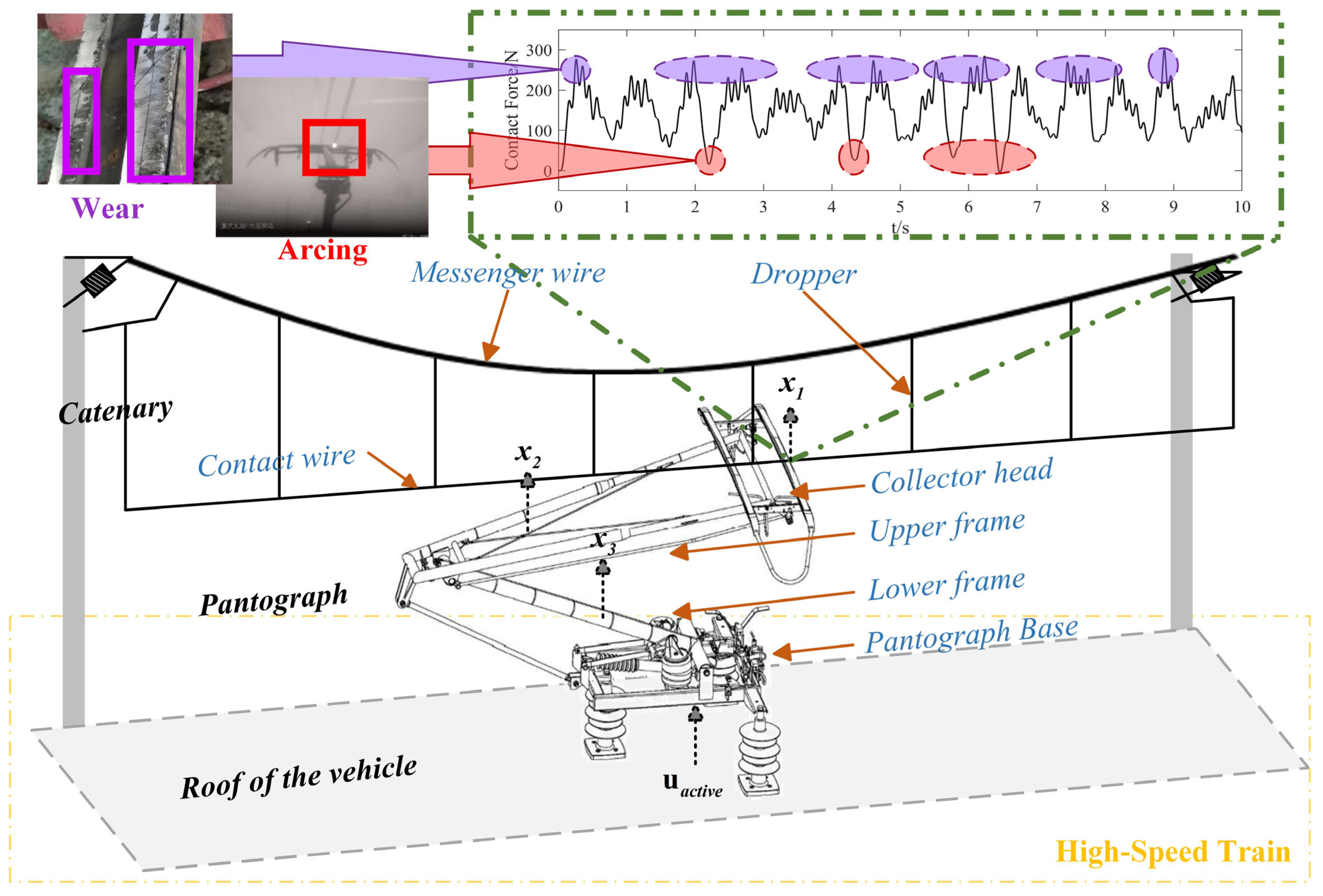
The pantograph–catenary interaction is one of the three main principal dynamic coupling relationships in high-speed systems [1], with contact behavior between the pantograph and the catenary critically influencing operational safety and economic efficiency. As the current collection apparatus, the pantograph may induce extreme contact force fluctuations during engagement with the catenary, leading to contact anomalies: excessive force accelerates wear on the collector head and catenary wire [2,3,4], potentially causing stripping or fractures, whereas insufficient force results in intermittent contact, producing abrupt voltage differentials that manifest as electrical arcing [5,6,7]. These adverse contact phenomena are shown in Figure 1. Traditional passive control approaches primarily focus on structural parameter optimization, which offers limited effectiveness with high implementation costs. Active control algorithms mitigate contact force oscillations by applying external forces to regulate the lift amplitude of the pantograph. This methodology not only delivers significantly enhanced control performance but also represents a software-driven solution with significant practical advantages.

Academically, research on active pantograph control algorithms mainly focuses on the improvement of traditional control methods. Al-Awad et al. [8] employed a genetic algorithm to optimize PID parameters on a reduced-order model, achieving smaller overshoot and a faster response. Still, the model is overly idealized and fails to capture the contact force dynamic characteristics arising from the real pantograph–catenary coupling situation. Farhan et al. [9] proposed a simplified fuzzy controller to reduce design complexity, demonstrating effective suppression of contact force oscillations; however, the simplified fuzzy rule set offers limited adaptability and lacks robustness guarantees against unknown disturbances. Song et al. [10] introduced a mechanical impedance-based PD sliding-mode surface design, theoretically reducing system impedance in the dominant contact-force frequency band, yet the switching gain depends on manual tuning without algorithmic optimization. Wang et al. [11] applied fractional-order modeling to the pantograph base air spring and used LQR via feedback linearization to handle time-varying stiffness in the pantograph–catenary coupling; nevertheless, the $\mathit{Q}$ and $\mathit{R}$ weight matrices remain empirically set up, without further validation of optimal performance. The foregoing studies reveal a common drawback of conventional active control algorithms, which all depend on experience-driven tuning of controller parameters.

In recent years, the deep reinforcement learning (DRL) algorithm, as a decision-making algorithm, has gained extensive application in control engineering [12,13,14]. Building on this approach, numerous studies have also emerged in the field of train control [15,16]. Wang et al. [17,18] pioneered the application of DRL to active pantograph control. Their work focuses on modifying DRL algorithms to accommodate the dynamic characteristics of pantograph–catenary systems, validating the method’s effectiveness in mitigating extreme oscillations of PCCF by training agents in simulation environments constructed with real-world railway-line parameters. Wang et al. [19] conducted further research on the feasibility of improved DRL algorithms for pantograph active control, based on the Deep Deterministic Policy Gradient (DDPG) framework. Sharma et al. [20], despite the “deep reinforcement learning” label, actually combined deep learning and traditional control: a Bi-LSTM network predicts contact force fluctuations to drive a fuzzy fractional PID controller, with Aquila optimization tuning parameters, offering a novel perspective for pantograph control. However, their deep-learning application centers on prediction and parameter optimization rather than genuine reinforcement learning. Leveraging its trial-and-error decision making, a DRL agent can function as a self-contained controller that autonomously learns corrective control forces to suppress extreme PCCF oscillations, thereby complementing and enhancing conventional control strategies.

Given that the pantograph can be modeled as a spring–damper system [21,22,23], its control strategy can draw on active suspension control methods used for similarly modeled vehicle suspensions, where LQR has been widely applied in automotive suspension and railway bogie control [24,25,26,27]. Accordingly, by introducing the Crowned Porcupine Optimization algorithm (CPO) to optimize the $\mathit{Q}$-weight matrix coefficients, optimal LQR feedback control actions are achieved. However, due to the coupled dynamics of the pantograph–catenary interaction, the PCCF still oscillates and remains significantly deviated from the target contact force [28,29] even under the LQR control situation. To address this issue, we designed an offline dual-model-based control law for secondary tuning of the LQR output, generating an ideal action distribution that brings the actual contact force closer to the target. However, since the dual-model strategy requires two controlled pantograph instances and cannot be directly deployed in a real-time system—and simply implementing the control law on a single-model pantograph would disrupt real-time LQR computation—we treat the tuned actions as “expert actions” and employ a combined imitation learning (IL) and DRL approach to learn the expert action distribution and online compensate the real-time CPO-LQR controller output. This enables, within a single-model framework, significant suppression of extreme contact force oscillations beyond the theoretical baseline.

Specifically, the main contributions of this paper are as follows:

• A CPO-LQR baseline controller is developed by optimizing the $\mathit{Q}$-weight matrix via the CPO algorithm, achieving strong PCCF suppression; its control outputs are further refined using an offline control law based on the dual pantograph–catenary model structure, resulting in expert actions that outperform the baseline and provide theoretically optimal control performance.
• To enhance practical applicability, a compensation control strategy is proposed by superimposing the offline expert force as well as the compensation force ${\mathbf{u}}_{comp}$ onto real-time CPO-LQR output ${\mathbf{u}}_{CPO-LQR}$, enabling an active controller based on a single pantograph–catenary model structure and yielding superior suppression of extreme oscillations.
• The compensatory action ${\mathbf{u}}_{comp}$ is trained using the BC-SAC algorithm, which embeds behavioral cloning loss into SAC to allow partial expert imitation while preserving the environment-driven interaction capabilities; an attenuation mechanism further balances exploration and imitation, leading to better performance than pure expert-based compensation.

This article is organized as follows: Section 2 establishes the pantograph–catenary coupling dynamic model and defines the control objectives; Section 3 presents the core control framework proposed herein; Section 4 provides simulation experiments and validations; and Section 5 lists the conclusion.

2. Preliminaries and Problem Formulation

To elucidate the dynamic characteristics of contact force during pantograph–catenary coupling and provide a basis for subsequent active control strategy design, this section first establishes a mathematical model of the pantograph–catenary interaction to accurately describe the system’s dynamic response under operating conditions. The model is then embedded in a Markov decision process (MDP) framework, defining the state and action spaces for the active pantograph control task and laying a formal foundation for compensatory controller design and training based on the DRL algorithm. To ensure that the control objectives are scientifically sound and comparable, this section also quantifies the target contact force and several performance metrics by standards [28,29], and designs corresponding objective and reward functions, providing quantitative criteria for training and simulation validation of the control strategies.

2.1. Mathematical Modeling of the Pantograph–Catenary Coupling System

The pantograph–catenary coupling model comprises two subsystems, which are the catenary system and the pantograph system. In this work, MATLAB/Simulink R2021b is used to model both the pantograph and the catenary system as the controlled plant for offline training and online validation of the control strategy.

The catenary is a complex, nonlinear structure that must be simplified for practical modeling. Following the approach in [30], we apply the following simplifications:

• Lateral vibration effects of the catenary are omitted. Although studies [31,32] have employed aerodynamic simulations and finite-element analyses to examine catenary lateral dynamics under abnormal conditions, our work focuses on vertical current collection and control algorithm design, since under normal operating conditions lateral contact-wire vibration is not a primary driver of current collection performance.
• The contact wire and messenger wire are modeled as Euler–Bernoulli beams with constant stiffness and tension.
• Adjacent anchor sections of the catenary are treated as independent subsystems.
• The mid-span of each dropper is represented by a spring element, as illustrated in Figure 2.

Thus, the simplified stiffness expression is derived by fitting the actual stiffness curve obtained from finite element analysis using least squares, from which the expression [30] can be written as follows:

$$k(t)=k_0\left[1+{\alpha }_1\cos \left({\displaystyle \frac{2\pi v}{L}}t\right)+{\alpha }_2\cos \left({\displaystyle \frac{2\pi v}{L_1}}t\right)+\right.\left.{\alpha }_3{\cos }^2\left({\displaystyle \frac{2\pi v}{L}}t\right)+{\alpha }_4{\cos }^2\left({\displaystyle \frac{\pi v}{L}}t\right)+{\alpha }_5{\cos }^2\left({\displaystyle \frac{\pi v}{L_1}}t\right)\right]$$

(1)

where $v$ is the operating speed of the train in units of m/s; $L$ is the span of the contact wire; $L_1$ is the distance between adjacent dropper lines; $k_0$ is the average stiffness of the catenary system; and ${\alpha }_i\left(i=1~5\right)$ are the stiffness coefficients of the catenary system, for which the values are ${\alpha }_1=0.4665$, ${\alpha }_2=0.0832$, ${\alpha }_3=0.2603$, ${\alpha }_4=-0.2801$, and ${\alpha }_5=-0.3364$. $L$ and $L_1$ are set to 50 m and 8 m, respectively, and $k_0$ is equal to 3694.5 N·m⁻¹.

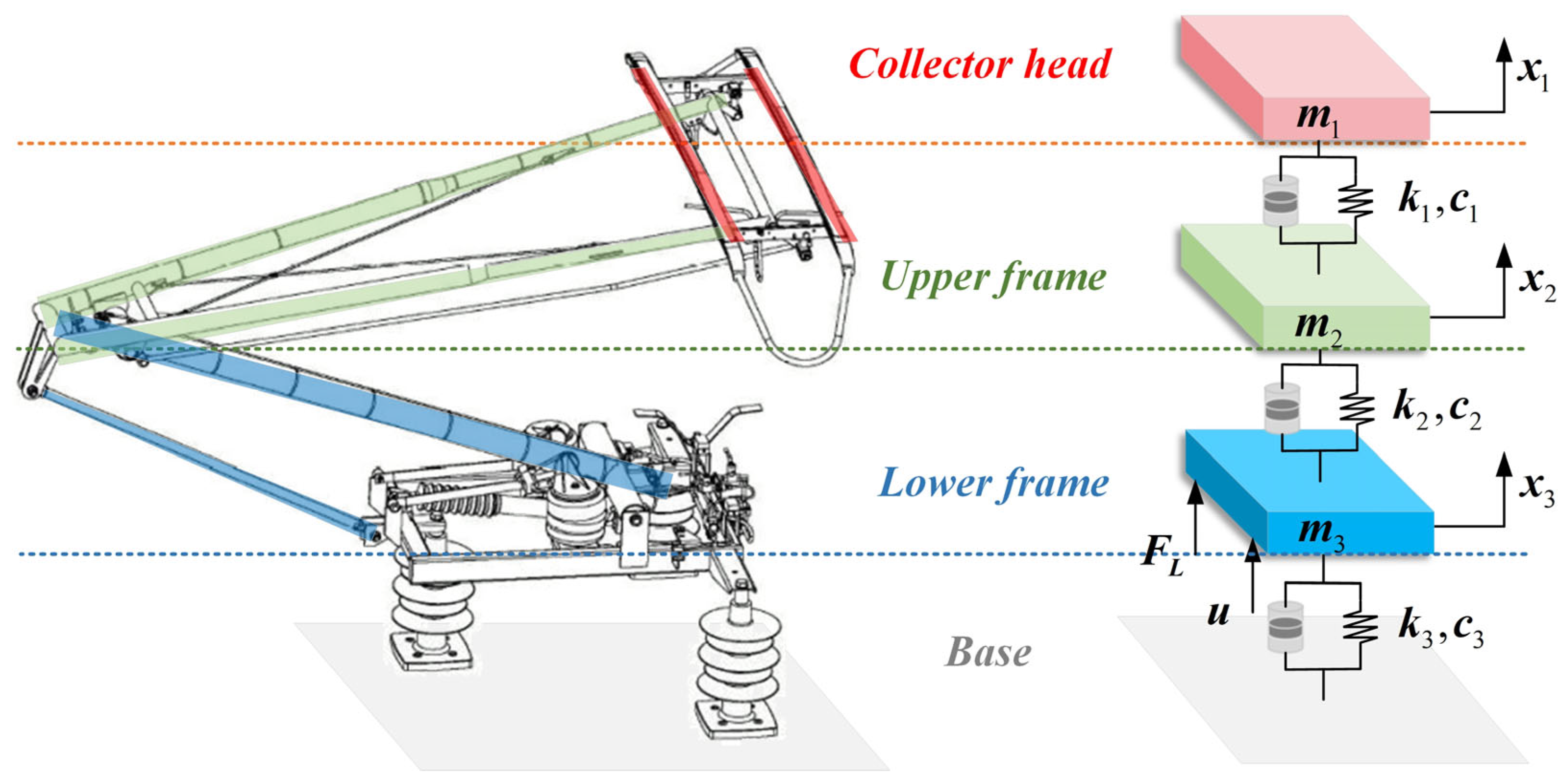
Numerous pantograph models have been developed for specific research objectives [33,34]. However, simpler approaches—such as the two-mass model in [8,11]—cannot fully capture the pantograph’s overall structural response. Therefore, we adopt a more comprehensive three-mass model to represent the pantograph’s three main components—the collector head, the upper frame, and the lower frame—as illustrated in Figure 3. The three-mass model is sufficient to characterize the pantograph’s dynamic behavior and has been validated in [22].

Based on the three-mass pantograph model, force analysis is performed, and for each mass, the dynamic differential equation is derived as follows:

$$\left\{\begin{array}{l}{m}_1{\ddot{x}}_1+c_1\left({\dot{x}}_1-{\dot{x}}_2\right)+k_1\left(x_1-x_2\right)=F_{pc}=k\left(t\right)x_1\hfill \\ m_2{\ddot{x}}_2+c_1\left({\dot{x}}_2-{\dot{x}}_1\right)+c_2\left({\dot{x}}_2-{\dot{x}}_3\right)+k_1\left(x_2-x_1\right)+k_2\left(x_2-x_3\right)=0\hfill \\ m_3{\ddot{x}}_3+c_2\left({\dot{x}}_3-{\dot{x}}_2\right)+c_3\left({\dot{x}}_3-{\dot{z}}_d\right)+k_2\left(x_3-x_2\right)+k_3\left(x_3-z_d\right)=F_L+u\left(t\right)\hfill \end{array}\right.$$

(2)

The above expressions can be arranged into the state-space function as follows:

$$\left\{\begin{array}{l}\dot{\mathit{x}}=\mathbf{A}\left(t\right)\mathit{x}+\mathbf{B}\mathit{u}+{\mathbf{G}}_1{F}_L+{\mathbf{G}}_2{w}_z\hfill \\ \mathit{y}=\mathbf{C}\mathit{x}+\mathbf{D}\mathit{u}\hfill \end{array}\right.$$

(3)

where $\mathit{x}={\left[x_1,{\dot{x}}_1,x_2,{\dot{x}}_2,x_3,{\dot{x}}_3\right]}^T$; $\mathit{u}=u\left(t\right)$; $x_i\left(i=1,2,3\right)$ represents the oscillatory displacement of the collector head, upper frame and lower frame of the pantograph, respectively; $F_L$ denotes the static uplift force; and $z_d$ is the disturbance transmitted from carriage oscillations to the pantograph base.

In this paper, we adopt the parameters of the high-speed pantograph type DSA380, where $m_i\left(i=1,2,3\right)$ are 7.12 kg, 6 kg, and 5.8 kg, respectively; $k_i\left(i=1,2,3\right)$ are 9430 N·m⁻¹, 14,100 N·m⁻¹, and 0.1 N·m⁻¹, respectively; and $c_i\left(i=1,2,3\right)$ are 0 N·s·m⁻¹, 0 N·s·m⁻¹, and 70 N·s·m⁻¹, respectively.

2.2. Markov Decision Process Modeling

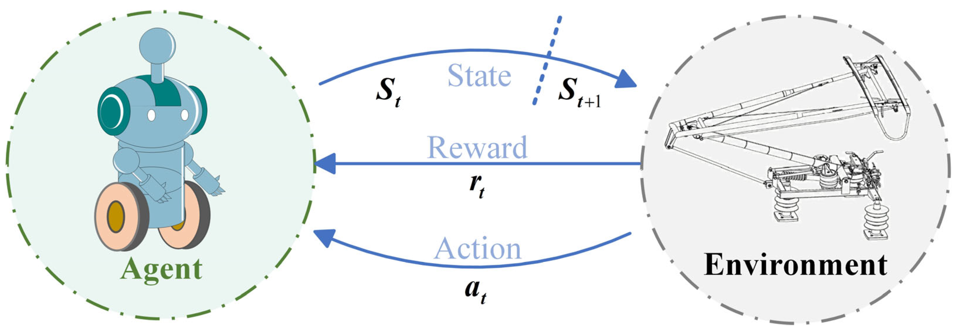
When formulating the active pantograph control problem as a Markov Decision Process (MDP), the state space and action space must be explicitly defined to enable the agent to make decisions based on current observations at each timestep while dynamically interacting with the environment, as illustrated in Figure 4. This section details the state space and control actions required for implementing the deep reinforcement learning-based active pantograph control algorithm.

2.2.1. State Space

The state should include sufficient information to characterize the current system dynamics and environmental disturbances, enabling the control policy to compensate for oscillations or deviations promptly. Assuming control is executed at discrete time steps $t=0$ s, $t=1$ s, $t=2$ s, $\dots$, the evolution of the pantograph–catenary coupling system state over each sampling period can be approximated as a Markov transition, where the next state depends only on the current state and the applied action. Therefore, the state space is defined as follows:

$$S_t=\left\{s|s_t=\left(F_{pc,t},F_{pc,t-1},F_{pc,t-2},\text{….},F_{pc,t-n+1}\right)\right\}$$

(4)

where $F_{pc,t}$ denotes the pantograph–catenary contact force. According to the first mass equation in (2), the contact force equals the variable stiffness coefficient of the catenary multiplied by the displacement of the collector head. Therefore, we directly focus on the state information of $F_{pc}$ rather than using $x_1$, adopting $F_{pc}$ as the primary controlled state variable to enable the agent to make more accurate control decisions.

2.2.2. Action Space

The agent’s action corresponds to the compensation force applied to the output of the real-time LQR controller by the proposed framework, denoted as ${\mathbf{u}}_{comp}$. Considering the actuator’s physical capabilities and safety limits, the compensation force must be restricted to the interval $\left[{\mathbf{u}}_{comp,\max },{\mathbf{u}}_{comp,\min }\right]$, and the agent selects actions within this range based on the observed state. To facilitate network training and output, we typically normalize the policy network’s raw output to $\left[-1,1\right]$, then use a linear mapping to obtain the actual compensation force value as follows:

$${\mathbf{u}}_{comp,t}=100\times a_t,A_{{\mathbf{u}}_{comp,t}}=\left\{a|a_t=\left[-1,1\right]\right\}\Rightarrow {\mathbf{u}}_{comp,t}\in \left[-100,100\right]$$

(5)

At each discrete-time period $T_s$, the agent observes the system state and outputs a normalized action. This action is mapped to a compensatory force ${\mathbf{u}}_{comp,t}$, which is superimposed on the baseline LQR controller output to form the composite control input. Within our framework, a one-dimensional continuous compensatory force suffices to suppress catenary force oscillations while reducing policy learning complexity.

2.3. Definition of the Objective Function and the Reward Function

In this subsection, the desired contact force state for the pantograph active control task is specified in detail based on international standards. On this basis, an objective function is designed for optimizing the $\mathit{Q}$-weight matrix coefficients of the LQR primary controller via the CPO algorithm, and the reward function is defined to guide policy learning for the compensatory controller trained by the DRL algorithm.

2.3.1. Specification of Performance Metrics

According to the Reference [17] and Standards [28,29], the target value of the desired contact force varies with train operating speed, as expressed by the following equation:

$$F_{pc,Trgt}=0.00097\times V^2+70$$

(6)

where $F_{pc,Trgt}$ denotes the target contact force, in the unit of N, and $V$ is the operating speed of the train, in the unit of km/h.

We define the control error $E_{pc}$ as the deviation between the controlled contact force $F_{pc,Ctrl}$ and the target contact force $F_{pc,Trgt}$, serving to assess how closely the controller drives the contact force toward its target value. Ideally, a smaller error indicates more effective suppression of extreme contact force fluctuations. The control error $E_{pc}$ is expressed as:

$$E_{pc}=\left|F_{pc,Ctrl}-F_{pc,Trgt}\right|$$

(7)

The standard deviation of the contact force is a key performance metric, as higher standard deviations reflect more extreme fluctuations. Ideally, this metric should be minimized. The acceptable range of the statistical contact force $F_{pc,Std}$ is calculated based on the standard deviation, which is defined as:

$$F_{pc,Std}=\left[F_m-3{\delta }_{STD},F_m+3{\delta }_{STD}\right]$$

(8)

where $F_m$ is the mean contact force and ${\delta }_{STD}$ is the standard deviation value as specified by standards [28,29].

Figure 5 delineates the variation trend of target contact force when train speeds exceed 300 km/h, while contrastingly presenting the statistically derived contact force ranges under passive control at different velocities (computed per (8)). Crucially, as velocity increases, the fluctuation range of contact forces exhibits notable expansion, indicating significant amplification of contact force oscillations.

2.3.2. Objective Function

The objective function drives the offline CPO algorithm’s search for optimal LQR solutions. Its design principles encompass a dynamic target contact force, permissible standard deviation ranges with safety thresholds, and a penalty mechanism for constraint violations. The objective of overarching is to minimize the standard deviation of the contact force as much as possible while satisfying safety and convergence requirements; if significant deviations from the target contact force or potentially unsafe force levels arise, penalty terms steer the optimization process away from suboptimal solutions. The specific formulation is as follows:

$$\begin{gathered} f=\left\{\begin{array}{ll}\underset{f_a}{\underbrace{{\displaystyle \frac{F_{pc,Std\_act}}{F_{pc,Std\_pass}}}}}+\underset{f_b}{\underbrace{{\displaystyle \frac{\left|0.97F_{pc,Trgt}-F_{pc,Mean}\right|}{0.03F_{pc,Trgt}}}}}+\underset{f_c}{\underbrace{10}},if\hfill & F_{pc,Std\_act}>F_{pc,Std\_pass}\left|\right|F_{pc,Std\_act}>F_{pc,Saftety}\left|\right| \\ {F}_{pc,Mean}>F_{pc,Trgt}\left|\right|F_{pc,Mean}<0.97F_{pc,Trgt}\\ \frac{F_{pc,Std\_act}}{F_{pc,Std\_pass}},else\hfill & \end{array}\right. \end{gathered}$$

(9)

where $F_{pc,Mean}$ denotes the mean contact force; $F_{pc,Std\_act}$ is the contact force standard deviation under active control; $F_{pc,Std\_pass}$ is the contact force standard deviation under passive control; and $F_{pc,Saftety}$ is the safety threshold for the contact force standard deviation, set to 30% of the mean contact force. The first term $f_a$ reflects the degree to which the fluctuations’ amplitude exceeds acceptable levels. The second term $f_b$ quantifies the deviation of the mean contact force from the target value, using an absolute value to capture deviations when the mean is above the target or below the lower bound. The third term $f_c$ is a fixed penalty: a constant +10 is added to assign a large fitness value to severe violations, guiding the optimization algorithm to avoid such solutions. When all constraints are satisfied, the fitness value is determined solely by the first term $f_a$. The optimization objective is thus reduced to minimizing this standard deviation to suppress contact force fluctuations while maintaining the mean contact force around the target value.

2.3.3. Reward Function

The reward function serves as the quantitative evaluation mechanism bridging agent–environment interactions, directly governing the convergence quality and ultimate performance of learned policies. Given that the primary objective of active pantograph control is to regulate uncontrolled contact force fluctuations around the target value, we consider the error metric as the absolute deviation between actual and target states to guide the policy exploration, formally expressed as:

$$R_t=-{\displaystyle \frac{\epsilon }{100}}{\left(F_{pc,t}-F_{pc,Trgt}\right)}^2$$

(10)

where $F_{pc,t}\in S_t$ denotes the environmental state variable; $F_{pc,Trgt}$ denotes the target contact force value; and $\epsilon$ serves as the weighting coefficient, equal to 0.5.

By penalizing the absolute error—whether the contact force overshoots or undershoots the target—with a negative reward, the agent is compelled to drive this error toward zero. Maximizing the cumulative reward thus directly corresponds to minimizing the contact force deviation. In the ideal scenario, when the measured force exactly equals the target, the absolute error vanishes and the total reward achieves its theoretical maximum of zero, indicating perfect fulfillment of the control objective.

3. CPO-LQR-BC-SAC Based Active Control Strategy

This section details the CPO-optimized LQR baseline controller and the corresponding offline control law for secondary tuning of the control actions, elaborates the rationale for behavioral cloning-based expert action imitation, and ultimately constructs a synergistic architecture between the CPO-LQR primary controller and the BC-SAC compensatory controller.

3.1. Overall Framework and Design Rationale

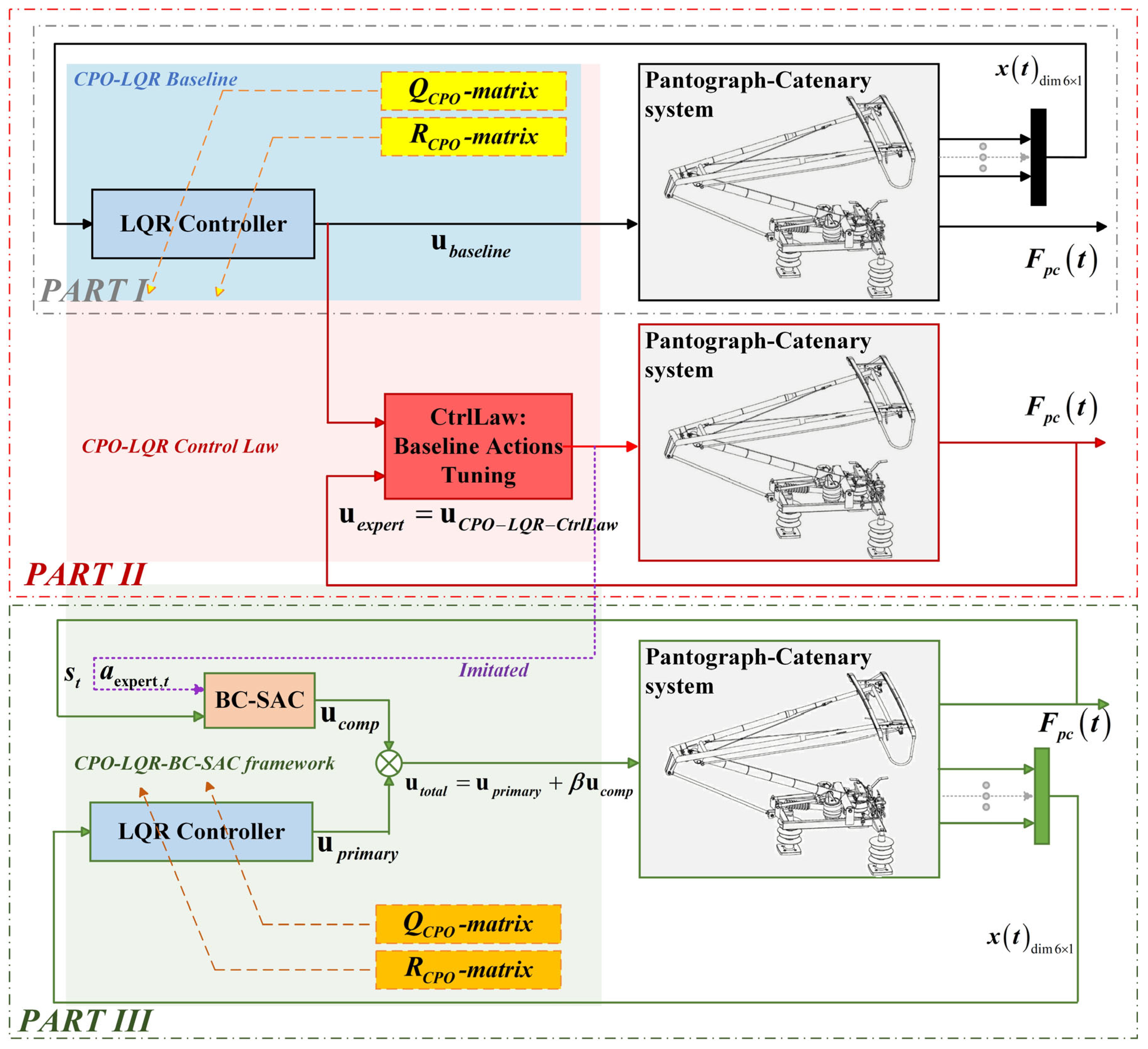
The design and implementation of the proposed control strategy consist of three main stages, as shown in Figure 6.

• Baseline Controller Construction—Part I:
  Use the CPO algorithm to offline-tune the LQR weight matrix, obtaining high-performance baseline control actions.
• Expert Action Refinement—Part II:
  Based on the dual pantograph–catenary model, design an offline control law (CPO-LQR-CtrlLaw) to perform a secondary optimization of the baseline actions, producing ideal control actions that surpass the baseline performance—these are treated as expert actions for the agent’s policy to imitate.
• Compensator Deployment—Part III:
  Given that standalone imitation learning or reinforcement learning controls cannot fully outperform the baseline controller, and that the dual-model approach faces practical deployment constraints, we conducted experiments that show superimposing real-time CPO-LQR outputs with the secondarily optimized control actions more effectively suppress extreme oscillations. Accordingly, a DRL compensator integrating imitation learning was constructed to replace the secondary optimization control actions. In the online test, the trained BC-SAC compensatory controller works in parallel with the baseline LQR; their outputs are weighted and combined to act on the pantograph–catenary system, enhancing fluctuation suppression and contact force dynamic performance.

The final execution mode of this framework operates via the closed-loop synergistic control architecture (Figure 6-Part III): Contact force states are synchronously input to both the CPO-LQR baseline controller and BC-SAC compensator through dual feedback pathways. Here, the baseline controller will be regarded as the primary controller. The BC-SAC algorithm generates compensatory actions ${\mathbf{u}}_{comp}$ based on real-time states, which are synthesized with the primary controller output ${\mathbf{u}}_{primary}$ to form the composite control input as ${\mathbf{u}}_{total}={\mathbf{u}}_{primary}+\beta {\mathbf{u}}_{comp}$. Meanwhile, the feedback variables fed into the CPO-LQR dynamically incorporate the contact-force response after compensation, forming a dynamically optimized closed loop together with the BC-SAC compensator.

3.2. Design of the Primary Controller Based on CPO-LQR

3.2.1. LQR Controller Baseline

According to the performance metrices described in Section 2.3, the LQR objective function is defined as follows:

$$J={\displaystyle \frac{1}{2}}{\displaystyle {\int }_0^{\infty }\left[x^T\left(t\right)\mathit{Q}x\left(t\right)+u^T\left(t\right)\mathit{R}u\left(t\right)\right]}$$

(11)

where $\mathit{Q}\in {ℝ}^{n\times n}$ is a semi-positive definite matrix, representing the impact of state deviation on the performance index; $\mathit{R}\in {ℝ}^{m\times m}$ is a positive definite matrix representing the impact of control inputs on the system’s energy consumption; and $x(t)=\mathbf{x}$ and $u(t)=\mathbf{u}$, which are determined based on the State-Space function of the pantograph–catenary coupling system given in (3) of Section 2.1.

To achieve optimal control performance in the pantograph–catenary system, it is essential to simultaneously minimize control energy expenditure and state deviation. Consequently, an optimal state-feedback control law is derived as follows:

$$\mathbf{u}=-\mathbf{K}x(t)$$

(12)

where $\mathbf{u}$ is the control input, specifically the active control force applied within the pantograph–catenary system; and $x(t)$ is the state vector. By optimal control theory, the feedback gain $\mathbf{K}$ is given by the following equation:

$$\mathbf{K}=-{\mathit{R}}^{-1}{\mathbf{B}}^{T}P$$

(13)

where $P$ is the symmetric matrix that satisfies the differential Riccati equation (DRE)—i.e., it is the solution corresponding to the state variable $\mathbf{x}$—based on which the state feedback gain $\mathbf{K}$ is obtained. The DRE is written as follows:

$$P\left(t\right)\mathbf{A}\left(t\right)+\mathbf{A}{\left(t\right)}^{T}P\left(t\right)-P\left(t\right)\mathbf{B}{\mathit{R}}^{-1}{\mathbf{B}}^{T}P\left(t\right)+Q=-\dot{P}\left(t\right)$$

(14)

In which $\mathbf{A}\left(t\right)$ and $\mathbf{B}$ are the state and input matrices of the pantograph–catenary coupled system defined in (3) of Section 2.1.

3.2.2. Optimization Method for the $\mathit{Q}$-Weight Matrix

The CPO algorithm was proposed by Abdel-Basset et al. [35] in 2024 as a swarm intelligence algorithm inspired by the defensive behavior of crowned porcupines. Comparative experiments on the CEC2017 benchmark show that CPO significantly outperforms various classical metaheuristic algorithms. Based on this, we employed CPO to optimize the $\mathit{Q}$-weight matrix of the LQR controller.

Specifically, CPO proceeds through global exploration and local exploitation phases. In the global exploration phase, quill-raising and acoustic-deterrence strategies enable broad sampling of the search space to prevent premature convergence. The local exploitation phase then uses odor-induced long jumps, along with leader-based mutation and crossover, to refine promising candidates and accelerate convergence. The two update rules correspond to (15) and (16), respectively:

$$x_i^{\left(t+1\right)}=x_t^{*}+a_0\left(r_1{x}_i^{\left(t\right)}-r_2{x}_p^{\left(t\right)}\right)+{\chi }_{0}N\left(0,1\right)$$

(15)

$$v_i^{\left(t\right)}=x_{r_1}^{\left(t\right)}+F_d\left(x_{r_2}^{\left(t\right)}-x_{r_3}^{\left(t\right)}\right),u_i^{\left(t\right)}=\left\{\begin{array}{ll}{v}_{i,j}^{\left(t\right)},if\hfill & ran{d}_j<C_{r}orj=j_{rand}\hfill \\ x_{i,j}^{\left(t\right)},else\hfill & \hfill \end{array}\right.$$

(16)

where $i=1,\dots ,N_p$, $N_p$ denotes the population size. In Equation (15), $x_t^{*}$ and $x_p^{\left(t\right)}$ denote the current global best and predator positions, while $r_1,r_2~U\left(0,1\right)$. In Equation (16), the index $j$ refers to the $j$th dimension, corresponding to the six weighting coefficients of the $\mathit{Q}$-matrix. The remaining hyperparameter definitions and values are listed in

Table 1. Hyperparameters of the CPO-LQR.

Description of Parameters	Symbols	Values
Population size	$N_p$	$200$
Maximum number of iterations	$T$	$30$
Cycle reduction period	$S_{cycle}$	$5$
Minimum population size	$N_{p_{\min }}$	$20$
Initial visual deterrence factor	$a_0$	$2$
Acoustic deterrence factor	${\chi }_0$	$0.1$
Differential evolution mutation factor	$F_d$	$5$
Crossover probability	$C_r$	$0.8$
Lévy flight distribution exponent	${\beta }_{levy}$	$1.5$
Upper bounds of the $\mathit{Q}$-weight matrix coefficients	$U_b$	$30$
Lower bounds of the $\mathit{Q}$-weight matrix coefficients	$L_b$	$0$

.

CPO’s strength lies in its superior global search capability, which allows it to thoroughly explore large solution spaces and avoid local optima. Leveraging this advantage, the algorithm performs deep optimization of the $\mathit{Q}$-matrix’s six weighting coefficients corresponding to the system’s state variables, identifying the optimal combination to maximize the suppression of pantograph–catenary contact force fluctuations and significantly enhance the overall control performance. Following the objective function designed in Section 2.3.2, the corresponding optimization mechanism is illustrated in Figure 7.

In summary, with the $\mathit{Q}$-matrix set to ${\mathit{Q}}_{CPO}$ obtained by CPO optimization and the $\mathit{R}$ matrix fixed as ${\mathit{R}}_{CPO}=\mathrm{diag}\left[1e^{-5}\right]$, the baseline control action ${\mathbf{u}}_{\mathit{baseline}}$ is computed as:

$${\mathbf{u}}_{\mathit{baseline}}=-{{\mathit{R}}_{\mathit{CPO}}}^{-1}{\mathbf{B}}^T{P}_{\mathit{CPO}}x\left(t\right)$$

(17)

3.2.3. The Offline Control Law

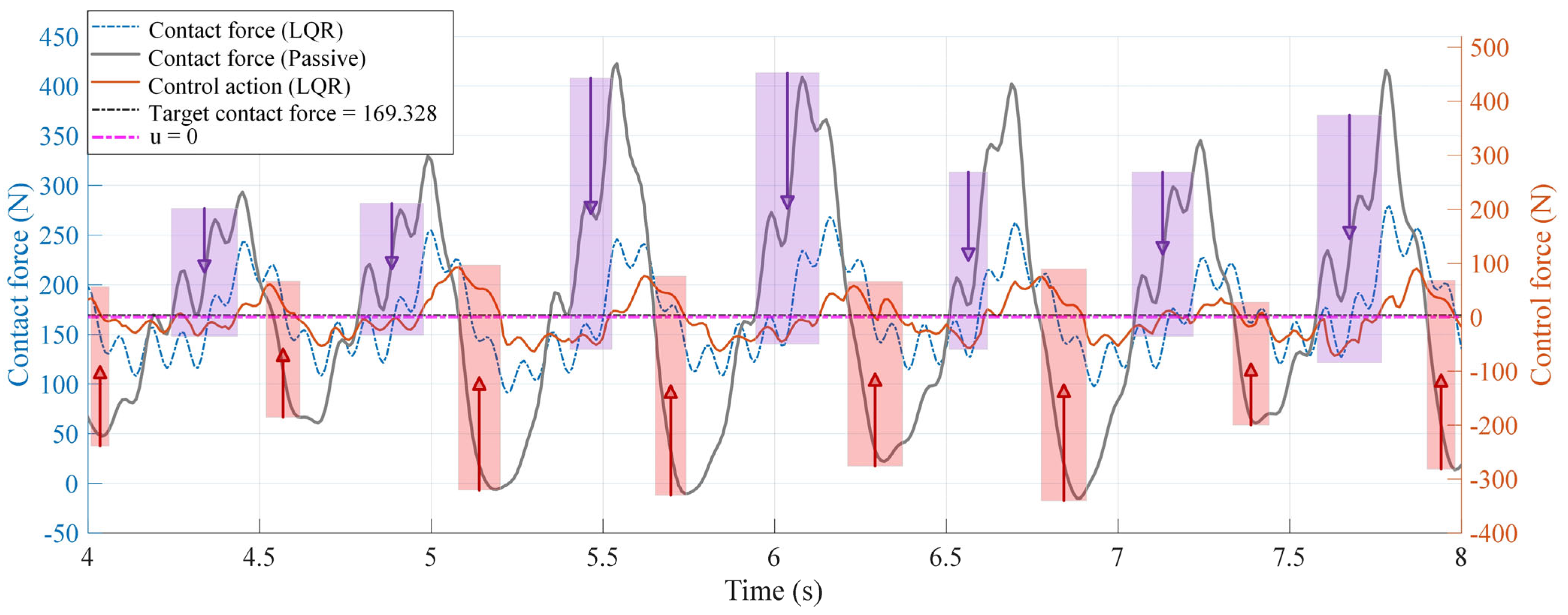
The experimental results indicate that the LQR control actions designed above exhibit the following characteristics: assuming a train speed of 320 km/h, the target contact force is 169.328 N as calculated in (6). At randomly selected instants $t=t_a\left(a=1,2,3,\dots \right)$, the uncontrolled contact force may reach 250 N; applying an active control force of −40 N to the pantograph system can reduce the contact force to about 180 N, driving it closer to the target. Similarly, at instants $t=t_b\left(b=1,2,3,\dots \right)$, the uncontrolled contact force may be 80 N; applying an active control force of +40 N can raise the contact force to about 150 N, also steering it toward the target. The control principle is illustrated in Figure 8.

Given the known distribution of effective CPO-LQR control actions, we designed a secondary control law to fine-tune these actions by applying incremental additions or subtractions, thereby achieving theoretically superior pantograph–catenary suppression performance compared to the baseline CPO-LQR controller. The offline control law is mathematically expressed as follows:

$${\mathrm{u}}_{CPO-LQR-CtrlLaw}=\left\{\begin{array}{lll}{\mathrm{u}}_{baseline}+\Delta u,\hfill & if& {\mathbf{u}}_{baseline}>0\&\&F_{pc,t}<F_{pc,Trgt}\\ {\mathbf{u}}_{baseline}-\Delta u,\hfill & if& {\mathbf{u}}_{baseline}<0\&\&F_{pc,t}>F_{pc,Trgt}\end{array}\right.$$

(18)

where $F_{pc,Trgt}$ denotes the target contact force under the current speed condition and $\Delta u$ is the increment value. $\Delta u$ should not be too large or too small; if it is too large, it may undermine the stability of the LQR controller, causing the control action to fail and the contact force to potentially diverge. If it is too small, it yields no additional effect and becomes indistinguishable from the baseline action. Based on experimental validation, we chose $\Delta u=25$ N.

The control system block diagram for the offline control law based on the dual model is shown in Figure 6 Part II. The effectiveness of this control law in suppressing the contact force compared to the baseline CPO-LQR will be validated through experimental results in Section 4.

3.3. Design of the Compensatory Controller Based on BC-SAC

Although CPO-LQR suppresses contact force significantly, it still deviates from the target, and the offline control law, despite its theoretical superiority, is impractical due to its reliance on the dual model. Therefore, a compensation control method is proposed to further enhance the control performance.

3.3.1. Soft Actor-Critic Algorithm

The core idea of the SAC algorithm is to maximize the cumulative reward while balancing exploration and exploitation by maximizing policy entropy. The inclusion of an entropy term gives it stronger exploration capabilities than other DRL algorithms in complex environments and prevents premature convergence to poor local optima, making it an excellent candidate for the MDP environment of this task. Its policy objective function can be expressed as follows:

$$J\left(\pi \right)=\underset{\pi }{\arg \max }{\displaystyle {\sum }_{t=0}^T{\mathbf{E}}_{\left(s_t,a_t\right)~\pi }}\left[r\left(s_t,a_t\right)+\alpha H\left(\pi \left(\cdot |s_t\right)\right)\right]$$

(19)

where $H\left(\pi \left(\cdot |s_t\right)\right)=-{\mathrm{E}}_{a~\pi }\left[\log \pi \left(a|s_t\right)\right]$ represents the entropy of the policy at state $s_t$, and $\alpha$ is the temperature coefficient that controls the trade-off between reward and entropy.

Accordingly, the update objective for the Actor network parameters $\theta$ is to produce actions that yield high Q-values while maintaining high entropy in the current state. Its loss function is expressed as follows:

$$L_{\pi }\left(\theta \right)={\mathbf{E}}_{s_t~D}\left[{\mathbf{E}}_{a_t~{\pi }_{\theta }\left(\cdot |s_t\right)}\left(\alpha \log {\pi }_{\theta }\left(a_t|s_t\right)-Q_{\psi }\left(s_t,a_t\right)\right)\right]$$

(20)

where $D$ denotes the replay buffer and $Q_{\psi }\left(s_t,a_t\right)$ is taken as the minimum of the two Critic network outputs to reduce overestimation. During updates, states $s_t$ are sampled from the buffer, actions $a_t$ are sampled from the current Actor, and the gradient of $L$ with respect to $\theta$ is computed for gradient descent, so that the policy improves in a direction that achieves both high value and sufficient randomness.

SAC employs two Q-networks $\left(Q_{\psi 1},Q_{\psi 2}\right)$ to reduce estimation bias. The Critic is updated based on the entropy-augmented Bellman target [36]:

$$y=r+\gamma {\mathbf{E}}_{a^{\prime }~\pi \left(\cdot |s_t^{\prime }\right)}\left[\underset{j=1,2}{\min }{Q}_{\psi j,\mathbf{target}}\left(s_t^{\prime },a_t^{\prime }\right)-\alpha \log \pi \left(a_t^{\prime }|s_t^{\prime }\right)\right]$$

(21)

And then minimizes the mean squared error:

$$L_Q\left({\psi }_i\right)={\mathbf{E}}_{\left(s_t,a_t,r_t,s_t^{\prime }\right)~D}{\left[Q_{\psi i}\left(s_t,a_t\right)-y\right]}^2,i=1,2$$

(22)

where $\mathit{\gamma }$ is the discount factor and the target Q-network parameters are slowly updated toward the main network via a soft-update mechanism:

$${\psi }_{\mathrm{target}1,2}\leftarrow \tau {\psi }_{1,2}+(1-\tau ){\psi }_{\mathrm{target}1,2}$$

(23)

The Critic update makes the Q-value estimates more accurate, providing a reliable evaluation signal for the Actor. After updating Actor and Critic, the temperature coefficient $\alpha$ is adjusted by minimizing L as follows:

$$L\left(\alpha \right)={\mathbf{E}}_{s_t~D}\left[{\mathbf{E}}_{a_t~{\pi }_{\theta }\left(\cdot |s_t\right)}\left(-\alpha \log {\pi }_{\theta }\left(a_t|s_t\right)-\alpha H\right)\right]$$

(24)

where $H$ is the desired minimum expected entropy.

3.3.2. Actor Network Integrated with Behavior Cloning

The behavior cloning method, first proposed by [37], is based on the core principle of constructing the loss between policy actions and expert actions and continuously minimizing it to approach zero, thereby guiding the policy network to generate outputs consistent with expert actions. In this study, the expert action ${\mathbf{u}}_{\mathrm{expert}}$ being mimicked corresponds to the ${\mathbf{u}}_{CPO-LQR-CtrlLaw}$ refined in Section 3.2.3.

However, the behavior cloning method relies solely on a single policy network and, unlike deep reinforcement learning algorithms, lacks a value network to evaluate the current policy. This limitation results in insufficient generalization to unseen states. Furthermore, during online testing, if the policy outputs deviations in unseen states, it may cause a shift in the state distribution. In continuous active control tasks for pantograph–catenary systems, this can lead to accumulated errors, potentially resulting in control failure.

To address this issue, we integrated the concept of behavior cloning into the update process of the deep reinforcement learning policy network by redesigning the loss function of the Actor network, which is expressed as follows:

$$L_{\pi }^{\prime }\left(\theta \right)={\mathbf{E}}_{s_t~D}\left[{\mathbf{E}}_{a_t~{\pi }_{\theta }\left(\cdot |s_t\right)}\left(\alpha \log {\pi }_{\theta }\left(a_t|s_t\right)-Q_{\psi }\left(s_t,a_t\right)\right)\right]+{\lambda }_n{L}_{BC}$$

(25)

where ${\lambda }_n$ represents the weighting coefficient, and $L_{BC}$ is the BC loss term, which is expressed as follows:

$$L_{BC}={\mathrm{E}}_{s_t~D}{‖\pi \left(s_t\right)-{\mathbf{u}}_{\mathrm{expert}}\left(s_t\right)‖}^2$$

(26)

We aim to further explore the potential for better control strategies beyond imitation, possibly surpassing the performance of expert actions. Therefore, a progressively decaying weighting coefficient is designed during the training process, expressed as follows:

$${\lambda }_n=\left\{\begin{array}{ll}1,\hfill & n\le {\displaystyle \frac{N}{2}}\hfill \\ {\displaystyle \frac{\frac{3N}{4}-n}{\frac{T}{4}}},\hfill & {\displaystyle \frac{N}{2}}\le n\le {\displaystyle \frac{3N}{4}}\\ \begin{array}{cc}0,& \end{array}\hfill & n\ge {\displaystyle \frac{3N}{4}}\end{array}\right.$$

(27)

where $N$ represents the total number of training episodes. In the initial $N/2$ episodes, imitation is emphasized to ensure the policy fully learns from expert experience. Subsequently, ${\lambda }_n$ gradually decays, reaching zero at $3N/4$, allowing the agent to engage in fully autonomous exploration on the established policy foundation to discover superior control strategies beyond the expert actions.

The method of integrating imitation learning with deep reinforcement learning through a hybrid loss function leverages expert action demonstrations to guide training while mitigating generalization risks inherent in pure behavioral cloning. By dynamically balancing imitation and autonomous exploration through gradual attenuation, it enhances the policy’s ability to further compensate for the actions of the primary controller.

3.4. Update Process of the Proposed Framework

After obtaining the optimal ${\mathit{Q}}_{CPO}$-weight matrix and expert action ${\mathbf{u}}_{expert}$, the proposed framework leverages these results to design and train a compensatory control policy agent. To clearly illustrate the update process of the active compensatory control policy within the CPO-LQR-BC-SAC framework, the pseudocode is presented as follows (Algorithm 1):

Algorithm 1. Pseudocode of the active pantograph compensation control algorithm based on the CPO-LQR-BC-SAC framework.

The CPO-LQR-BC-SAC Framework

Input:

Environment $\mathit{E}$ of the pantograph–catenary coupling system.

$\mathrm{Optimized}{\mathit{Q}}_{CPO}$-weight matrix and fixed ${\mathit{R}}_{CPO}$-weight matrix.

$\mathrm{Expert}\mathrm{action}{\mathbf{u}}_{expert}$ tuned by the offline control law.

$\mathrm{Actor}\mathrm{policy}{\pi }_{\theta }$$\mathrm{and}\mathrm{Critic}\mathrm{networks}{Q}_{{\psi }_{1,2}}$$\mathrm{with}\mathrm{target}\mathrm{networks}{Q}_{{\psi }_{\mathrm{target}1,2}}$.

Replay Buffer $D$.

Behavior-cloning weight decay schedule ${\lambda }_n$.

Output:

Trained compensatory policy ${\pi }_{\theta }$.

Procedure:

1. Initialization:

Randomly initialize Actor parameters $\theta$.

$\mathrm{Randomly}\mathrm{initialize}\mathrm{Critic}\mathrm{parameters}{\psi }_{1,2}$$\mathrm{and}\mathrm{set}\mathrm{target}\mathrm{networks}\text{: }{\psi }_{\mathrm{target}1,2}$.

Initialize temperature coefficient $\alpha$.

Initialize the replay buffer $D$ as empty.

Initialize behavior-cloning weight ${\lambda }_n$.

2. for episode = 1 to  $N$ do

$\text{3. Reset environment; obtain initial state }{s}_t\leftarrow s_{t=0}$.

4.         for step = 1 to M do

$\text{5. }\mathrm{Compute}\mathrm{the}\mathrm{action}\mathrm{of}\mathrm{the}\mathrm{primary}\mathrm{controller}\text{: }{\mathbf{u}}_{primary}=-{\mathbf{K}}_{CPO}{s}_t$.

$\text{6. }\mathrm{Obtain}\mathrm{expert}\mathrm{action}\mathrm{for}\mathrm{this}\mathrm{state}\text{: }{a}_{expert,t}{=\mathbf{u}}_{expert}~{\mathbf{u}}_{CPO\text{-}LQR\text{-}CtrlLaw}\left(s_t\right)$.

$\text{7. }\mathrm{Sample}\mathrm{compensatory}\mathrm{action}\mathrm{from}\mathrm{Actor}\text{: }{a}_t={\mathbf{u}}_{comp}\sim {\pi }_{\theta }\left(\cdot |s_t\right)$.

$\text{8. }\mathrm{Form}\mathrm{and}\mathrm{execute}\mathrm{total}\mathrm{action}\text{: }{\mathbf{u}}_{total}={\mathbf{u}}_{primary}+\beta {\mathbf{u}}_{comp}$.

$\text{9. }\mathrm{Interact}\mathrm{with}\mathrm{the}\mathrm{environment}\text{: }\mathrm{observe}\mathrm{next}\mathrm{state}{s}_t^{\prime }$$,\mathrm{reward}{r}_t$, and done.

$\text{10. }\mathrm{Store}\mathrm{transition}(s_t$$,a_t$$,a_{expert,t}$ $,r_t$$,s_t^{\prime }$, done) into D.

$\text{11. }{s}_t\leftarrow s_t^{\prime }$.

12.               if size(D) ≥ batch size, then:

13.                       Sample size per batch B from D.

14.                       Update Critic networks using the entropy-augmented Bellman targets                             based on (21) and (22).

15.                       Compute current behavior-cloning weight ${\lambda }_n$ based on (27).

16.                       Update Actor network based on (25) and (26).

17.                       Soft-update target Critic network parameters ${\psi }_{\mathrm{target}1,2}$ based on (23).

18.                       Update temperature parameter $\alpha$ based on (24).

19.               if done break

20.         end for

21. end for

$\mathbf{Return}\mathrm{policy}{\pi }_{\theta }$.

The updated process of the proposed framework is shown in Figure 9.

4. Experimental Validation and Result Analysis

In this section, based on the pantograph–catenary coupling model established in Section 2.1 and the performance metrics defined in Section 2.3.1, we conduct a detailed comparative analysis and validate the effectiveness of the proposed active compensation control framework. We present the training and testing results of both the primary controller and the compensatory controller, and illustrate the control performance of the control schemes under various speed conditions.

4.1. Hyperparameter Settings

Table 1 summarizes the definitions and values of the hyperparameters used in the CPO-optimized LQR primary controller.

For the BC-SAC algorithm, which is used to train the compensatory control policy, the hyperparameters are listed in

Table 2. Hyperparameters of the BC-SAC.

Description of Parameters	Symbols	Values
Discount factor	$\gamma$	$0.99$
Soft update rate	$\tau$	1 × 10−2
Learning rate	$lr$	2 × 10−4
Number of network layers	$layers$	$4$
Number of neurons	$neurons$	$512$
Activation function	$ReLU$	$-$
Optimizer	$Adam$	$-$
Maximum number of episodes	$N$	2 × 103
Maximum iterations of each step	$M$	1.5 × 102
Compensatory controller weight factor	$\beta$	$1.2$
Simple size per batch	$B$	$256$
Replay buffer	$D$	$20,000$

.

The detailed parameters of the pantograph and catenary used in the validation are provided in Section 2.1. All experiments were conducted on a host configured with an Intel(R) Core(TM) i7-10700F CPU @2.90 GHz (Intel Corporation, Santa Clara, CA, USA), NVIDIA GeForce RTX 3080 (NVIDIA Corporation, Santa Clara, CA, USA), and 16 GB of RAM; software interaction was facilitated by PyCharm 2022 with MATLAB/Simulink R2021b, and the core algorithms were built within the PyTorch 1.13.1+cu116 environment constructed on the Python 3.9 interpreter.

4.2. Control Performance of the Baseline Controller

As the baseline control method in the proposed framework, the control performance of CPO-LQR must be optimal to highlight the value of the compensatory control policy, i.e., to further improve upon a fully exploited baseline. This subsection presents a comparative validation of the proposed CPO-LQR and CPO-LQR-CtrlLaw.

4.2.1. Training and Testing Results

From Figure 5 discussed above, when the train operates above 300 km/h, the pantograph–catenary contact force exhibits severe oscillations. Therefore, we select four speed conditions—320 km/h, 340 km/h, 360 km/h, and 380 km/h—to optimize the corresponding $\mathit{Q}$-weight matrix for each case. To highlight the superiority of the CPO algorithm over other classical metaheuristic methods, we compare CPO with the genetic algorithm (GA) and the particle swarm optimization algorithm (PSO) used in References [24,25,26] under identical parameter settings. The convergence curves of the three algorithms for each speed condition are presented in Figure 10.

Figure 10 shows that the CPO algorithm exhibits the best overall convergence performance. Specifically, although PSO converges fastest among the three algorithms, it also settles at the highest final fitness value, indicating inferior exploration due to premature convergence. GA converges faster than CPO but still ends with a higher final fitness value; it enters a steady state in fewer iterations, risking entrapment in local optima. In the figure, GA’s final fitness matches CPO’s only at 360 km/h, while at all other speeds its final values remain higher than CPO’s. Owing to its four-stage exploration mechanism, CPO maintains a broad search scope, which naturally results in relatively slower convergence but ultimately contributes to achieving the lowest final fitness value, demonstrating the optimality of its optimization results. This indicates that, with identical parameter settings, CPO can discover more optimal $\mathit{Q}$-weight matrix coefficients, resulting in superior control performance. The optimized $\mathit{Q}$ values for each speed condition are summarized in

Table 3. $\mathit{Q}$-weight matrices optimized by the CPO algorithm under different speed conditions.

Speed Conditions	$\mathit{Q}$-Weight Matrices
320 km/h	${\mathit{Q}}_{CPO-320}=\mathrm{diag}\left[\begin{array}{llllll}25.1192\hfill & 1.7833\hfill & 22.5689\hfill & 0.3133\hfill & 30\hfill & 4.55\hfill \end{array}\right]$
340 km/h	${\mathit{Q}}_{CPO-340}=\mathrm{diag}\left[\begin{array}{llllll}27.1600\hfill & 1.7328\hfill & 30\hfill & 3.1496\hfill & 21.3052\hfill & 2.2465\hfill \end{array}\right]$
360 km/h	${\mathit{Q}}_{CPO-360}=\mathrm{diag}\left[\begin{array}{llllll}3.3080\hfill & 1.3131\hfill & 26.5692\hfill & 0\hfill & 28.1257\hfill & 14.2214\hfill \end{array}\right]$
380 km/h	${\mathit{Q}}_{CPO-380}=\mathrm{diag}\left[\begin{array}{llllll}29.3968\hfill & 1.0526\hfill & 2.4655\hfill & 0\hfill & 30\hfill & 8.2777\hfill \end{array}\right]$

.

Table 3 shows that the CPO-tuned $\mathit{Q}$-weight matrices vary in all six diagonal weight coefficients across speeds, with no uniform trend. This variability indicates that CPO adapts each controller’s emphasis to the specific dynamic behavior at each speed. Such flexibility ensures that the baseline LQR is optimally matched to its operating condition before applying the matrices.

By loading the trained $\mathit{Q}$-weight matrix into the LQR controller, we conducted online tests at all four speed conditions and compared three control strategies, passive Control, empirically tuned LQR, and CPO-LQR. In the empirical LQR method, the $\mathit{Q}$ and $\mathit{R}$ matrices are set according to Reference [11], with ${\mathit{Q}}_{emp}=\mathrm{diag}\left[1000,0,0,0,0,0\right]$, ${\mathit{R}}_{emp}=\mathrm{diag}\left[1\times {10}^{-7}\right]$.

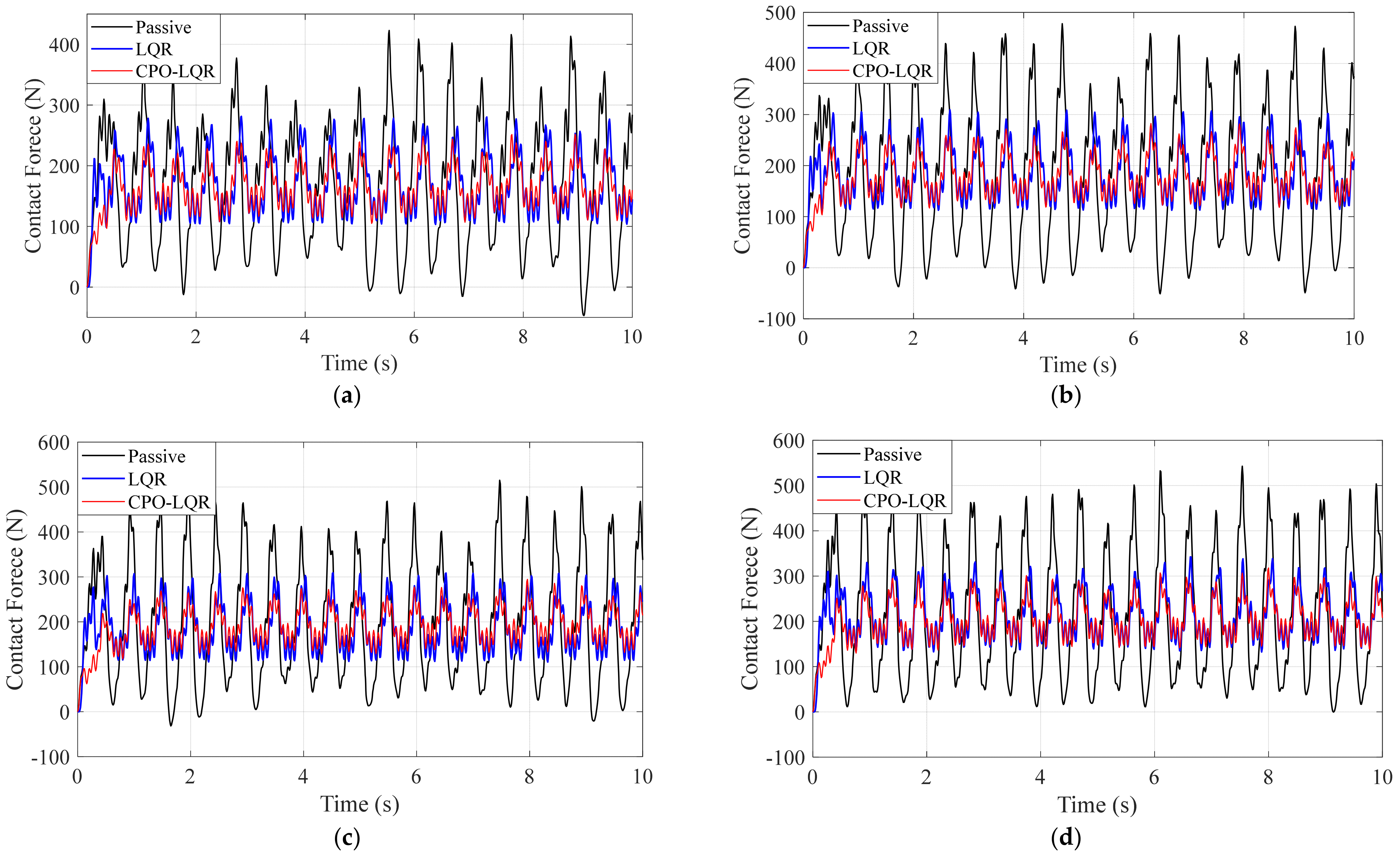
Figure 11 illustrates the control performance of the three control strategies across four speed conditions. The experimental results show that the CPO-optimized controller consistently and markedly reduces oscillation amplitudes in all cases. Compared to the uncontrolled case (Passive Control) and the empirically tuned LQR controller, CPO-LQR yields significantly lower force peaks as well as higher force valleys, demonstrating the smallest contact force fluctuation and superior contact force suppression performance.

4.2.2. Comparative Validation with the Offline Control Law

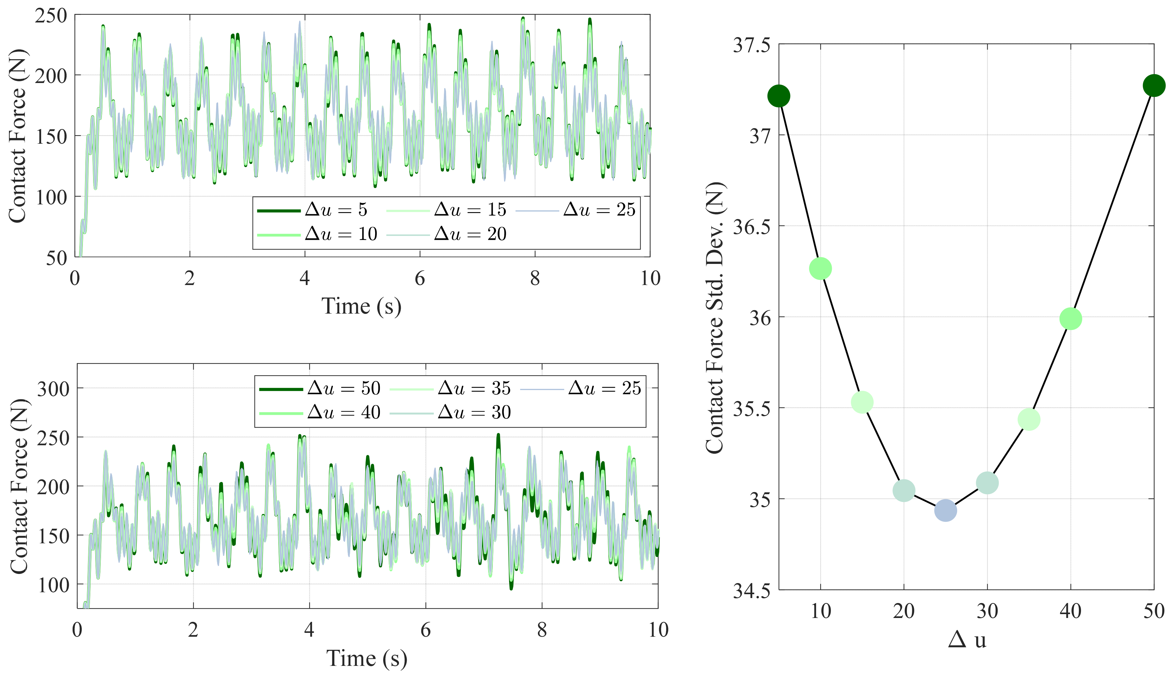
As mentioned earlier, the value of $\Delta u$ significantly affects the performance of the control law. We validated a range of $\Delta u$ in $\left[0,50\right]$ N to identify the optimal increment value.

As shown in Figure 12, when the increment value $\Delta u$ is below 25 N, the control action converges toward the baseline controller, yielding diminishing improvements. This behavior is expected because, per (18), as $\Delta u$ approaches zero, the correction term vanishes and the controller effectively reduces to ${\mathbf{u}}_{baseline}$, offering no noticeable advantage. Conversely, values of $\Delta u$ above 25 N lead to excessive corrections and degraded performance rather than further improvement. This trend is reflected in the curve of the contact force standard deviation: both very small and very large $\Delta u$ values increase the standard deviation and thus are reflected as the larger contact force oscillation amplitude. The minimum standard deviation occurs at $\Delta u=25$ N, indicating that this increment yields the best overall control performance.

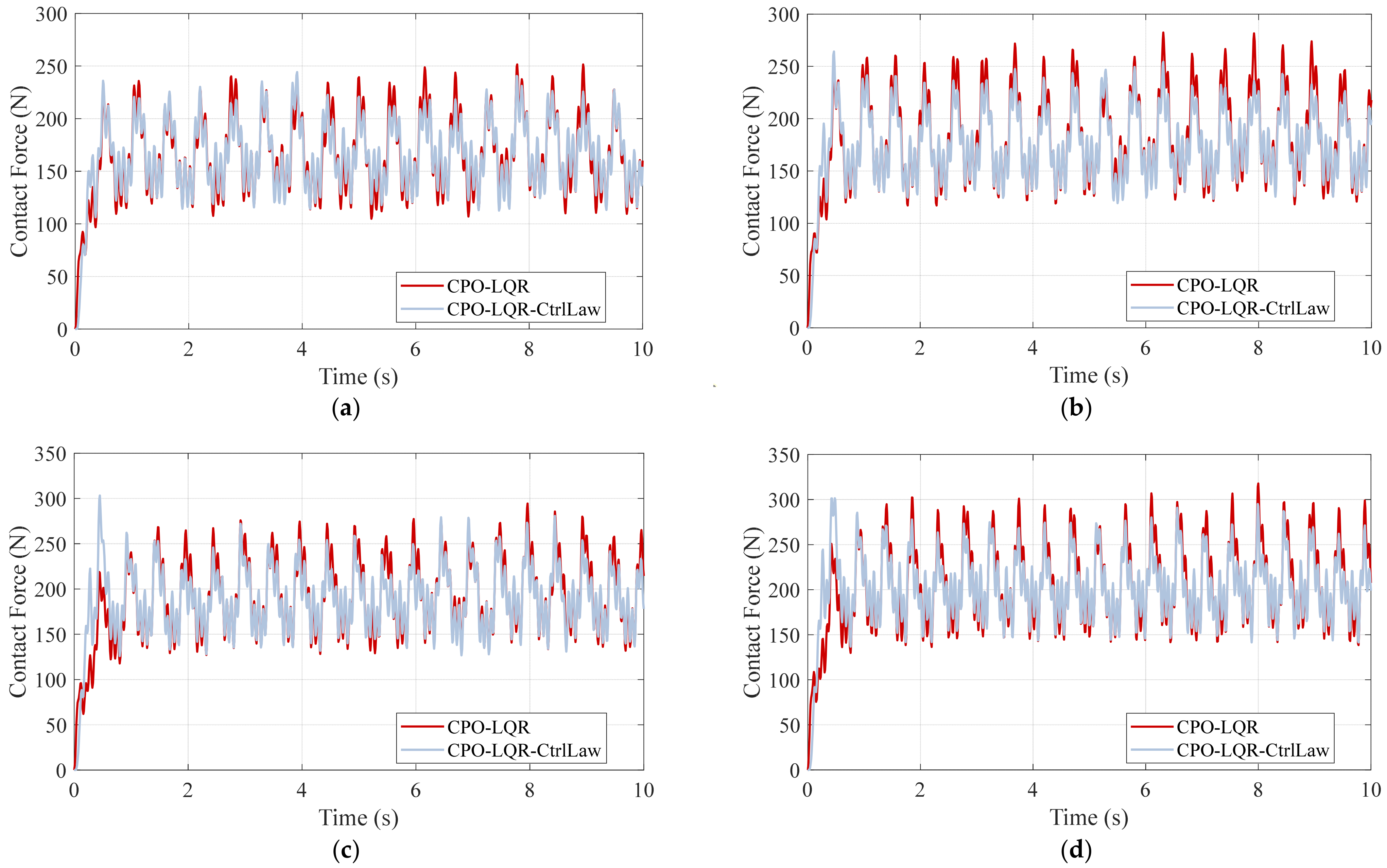
We then validated the dual model-based secondary-tuning control law CPO-LQR-CtrlLaw method under the same four speed conditions, as shown in Figure 13.

As shown in Figure 13, the experimental results indicate that the CPO-LQR-CtrlLaw not only reduces the excessive peaks of the contact force waveform but also raises the deep troughs, bringing both extreme contact force situations closer to the corresponding target contact value under all four speed conditions. Consequently, the secondarily adjusted baseline actions further enhance overall suppression of the contact-force fluctuations, confirming that the CPO-LQR CtrlLaw method outperforms the baseline CPO-LQR controller.

4.3. Control Performance of the Proposed Framework

Building upon the aforementioned baseline controller and the control law method, we further validated the online performance of the proposed unified compensation control framework, examining both its convergence behavior during training and its suppression effectiveness on contact force under different speed conditions in online testing.

4.3.1. Training and Testing Results

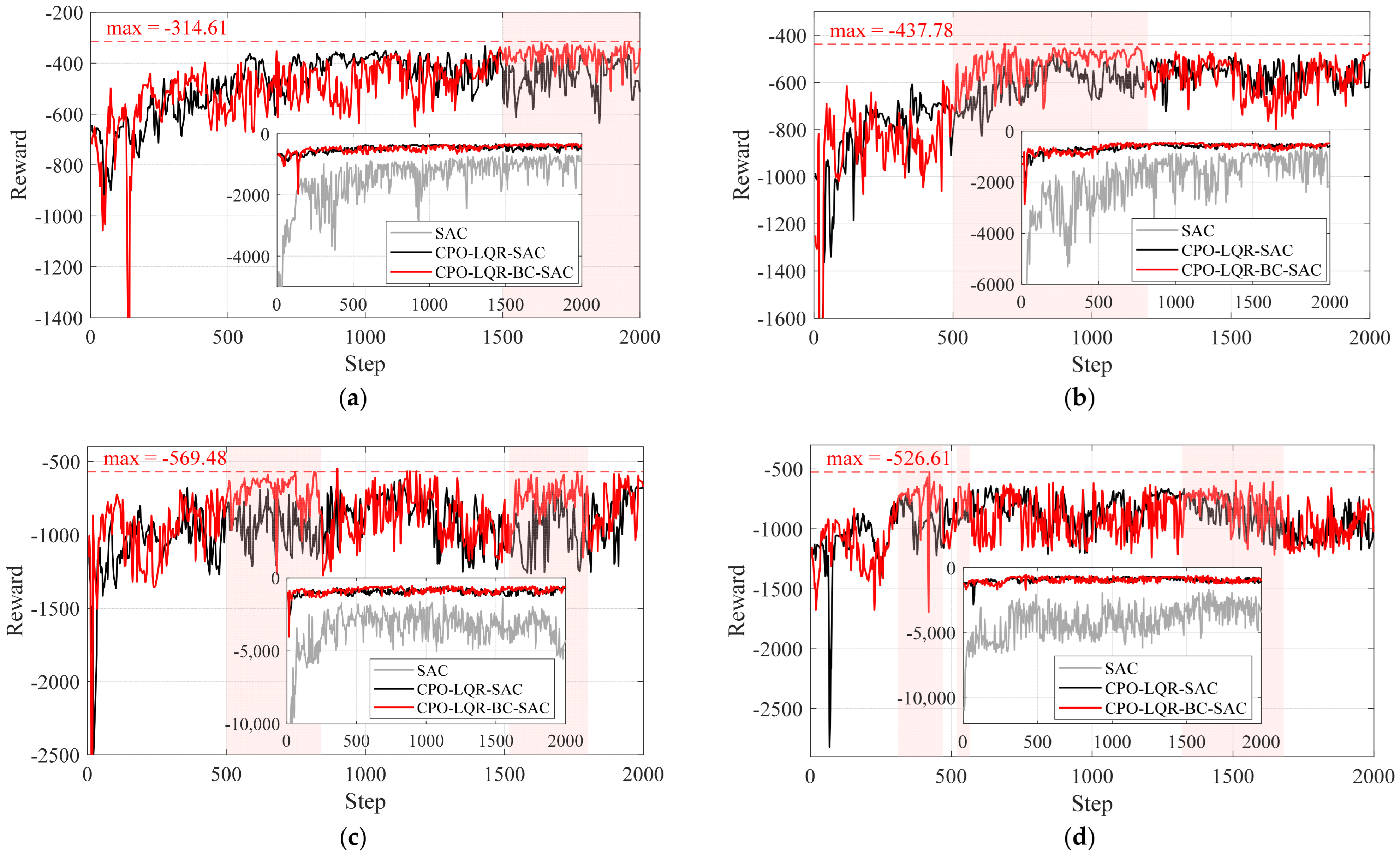
To comprehensively evaluate the contribution of each module in the proposed framework to control performance, we compared three schemes: the standalone SAC, the combined framework with CPO-LQR as the primary controller and the SAC as the compensatory controller, and the proposed framework with the added behavior-cloning loss term. Their reward convergence curves are shown in Figure 14.

Regardless of speed, the standalone SAC algorithm exhibits the worst convergence: its reward curve fluctuates wildly and settles at the lowest final value, indicating failure to explore an optimal policy. When SAC compensation is grafted onto the CPO-LQR baseline at 320 km/h, fluctuations are damped, but the peak reward stalls and even declines after roughly 800–1200 episodes, failing to continue improving. In contrast, CPO-LQR-BC-SAC, which integrates behavior cloning, demonstrates a consistently increasing reward trend over 2000 episodes and reaches the highest final reward. This advantage persists at higher speeds: at 340 km/h, it converges to a significantly higher reward between episodes 500 and 1200; at 360 km/h, it outperforms in two distinct bands (episodes 500–840 and 1515–1800); and at 380 km/h, it remains superior over episodes 310–470, 520–565 and 1320–1680. These findings demonstrate that adding behavior cloning effectively guides the agent toward targeted exploration in the policy space, enhancing learning stability and ultimately discovering superior control strategies. It is worth noting that the reward curves at 360 km/h and 380 km/h are more volatile than at lower speeds—a reasonable outcome given that contact-force oscillations intensify with train velocity.

The online test results for all speed conditions are presented in Figure 15. The standalone SAC policy fails to outperform the baseline CPO-LQR at any speed. However, when SAC is employed as a compensator alongside the CPO-LQR primary controller, the fluctuation suppression performance is significantly enhanced, as demonstrated by reduced oscillation amplitudes and less control errors across all four speed conditions. Furthermore, with the addition of the BC guided, the proposed framework achieves the best performance among the four methods—exhibiting the lowest oscillation amplitude and the smallest deviation from the target contact force—thereby fully confirming its superiority.

4.3.2. Comparative Validation Based on Expert Action Compensation

As previously described, to address the impracticality of deploying the dual-model offline control law directly, we propose superimposing the secondarily tuned baseline control actions onto the real-time CPO-LQR outputs, thereby achieving performance beyond that of standalone CPO-LQR. These tuned actions are treated as expert demonstrations for subsequent behavior cloning. In order to validate the effectiveness of expert action compensation and to demonstrate that the proposed framework outperforms pure expert action imitation, Figure 16 compares the performance of four control schemes under the 320 km/h, 340 km/h, 360 km/h, and 380 km/h conditions. Here, Expert-Compensated CPO-LQR (ECCPO-LQR) refers to the control framework that relies entirely on ${\mathbf{u}}_{expert}$-based compensation.

The experimental results in Figure 16 demonstrate that the ECCPO-LQR scheme significantly outperforms the CPO-LQR baseline and closely matches the performance of the ideal CPO-LQR-CtrlLaw. Hence, using these generated actions as “expert demonstrations” for behavior cloning is well justified. Furthermore, across all speed conditions, the CPO-LQR-BC-SAC framework not only retains the strengths of the expert demonstrations but, through autonomous exploration in deep reinforcement learning, surpasses both the CPO-LQR-CtrlLaw and ECCPO-LQR schemes. These results empirically demonstrate the effectiveness of our proposed active compensation control architecture, with imitation learning as its foundation and adaptive exploration enabling performance gains beyond the baseline.

4.4. Performance Evaluation

This subsection first conducts a comparative analysis of the proposed framework against various control algorithms under different speed conditions. Subsequently, to further verify its robustness, the trained control strategy is transferred to two additional pantograph types for testing, and its performance retention is evaluated.

4.4.1. Speed Range Performance Evaluation and Comparative Validation

Using the performance metrics defined in Section 2.3.1, we quantitatively compared the online test results of all control schemes discussed in this paper. The statistical summary of the control performance is presented in

Table 4. Summary of control performance metrics for different schemes at different speeds.

Speeds	Schemes	${\mathit{\delta }}_{\mathit{S}\mathit{T}\mathit{D}}$	Pct. Decline	${\mathit{E}}_{\mathit{p}\mathit{c}\_\mathit{a}\mathit{v}\mathit{g}}$	Pct. Decline
320 km/h	Passive Control	108.47	-	92.86 N	-
	LQR	48.38	55.40%	41.12 N	55.71%
	SAC	37.20	65.71%	27.76 N	70.10%
	CPO-LQR	34.38	68.30%	28.86 N	68.93%
	CPO-LQR-CtrlLaw	30.07	72.28%	25.52 N	72.52%
	ECCPO-LQR	32.24	70.28%	27.62 N	70.25%
	CPO-LQR-SAC	24.33	77.58%	19.94 N	78.52%
	CPO-LQR-BC-SAC	22.77	79.01%	18.68 N	79.87%
340 km/h	Passive Control	137.79	-	118.98 N	-
	LQR	52.62	61.81%	44.62 N	62.51%
	SAC	45.33	67.10%	32.18 N	72.95%
	CPO-LQR	39.48	71.35%	32.86 N	72.38%
	CPO-LQR-CtrlLaw	31.43	77.19%	27.10 N	77.22%
	ECCPO-LQR	34.01	75.32%	30.24 N	74.58%
	CPO-LQR-SAC	28.79	79.11%	23.98 N	79.85%
	CPO-LQR-BC-SAC	27.08	80.35%	22.44 N	81.15%
360 km/h	Passive Control	137.72	-	118.68 N	-
	LQR	54.54	60.40%	48.70 N	58.96%
	SAC	51.46	62.63%	39.26 N	66.92%
	CPO-LQR	38.25	72.22%	32.90 N	72.27%
	CPO-LQR-CtrlLaw	32.23	76.60%	27.12 N	77.15%
	ECCPO-LQR	34.40	75.02%	30.12 N	74.61%
	CPO-LQR-SAC	33.80	75.46%	28.06 N	76.35%
	CPO-LQR-BC-SAC	30.98	77.50%	26.52 N	77.66%
380 km/h	Passive Control	144.75	-	126.06 N	-
	LQR	52.44	63.78%	44.68 N	64.56%
	SAC	52.05	64.04%	42.04 N	66.66%
	CPO-LQR	41.65	71.23%	35.92 N	71.51%
	CPO-LQR-CtrlLaw	32.71	77.40%	27.24 N	78.39%
	ECCPO-LQR	36.18	75.01%	30.86 N	75.53%
	CPO-LQR-SAC	34.10	76.44%	28.70 N	77.23%
	CPO-LQR-BC-SAC	31.68	78.11%	26.48 N	78.99%

.

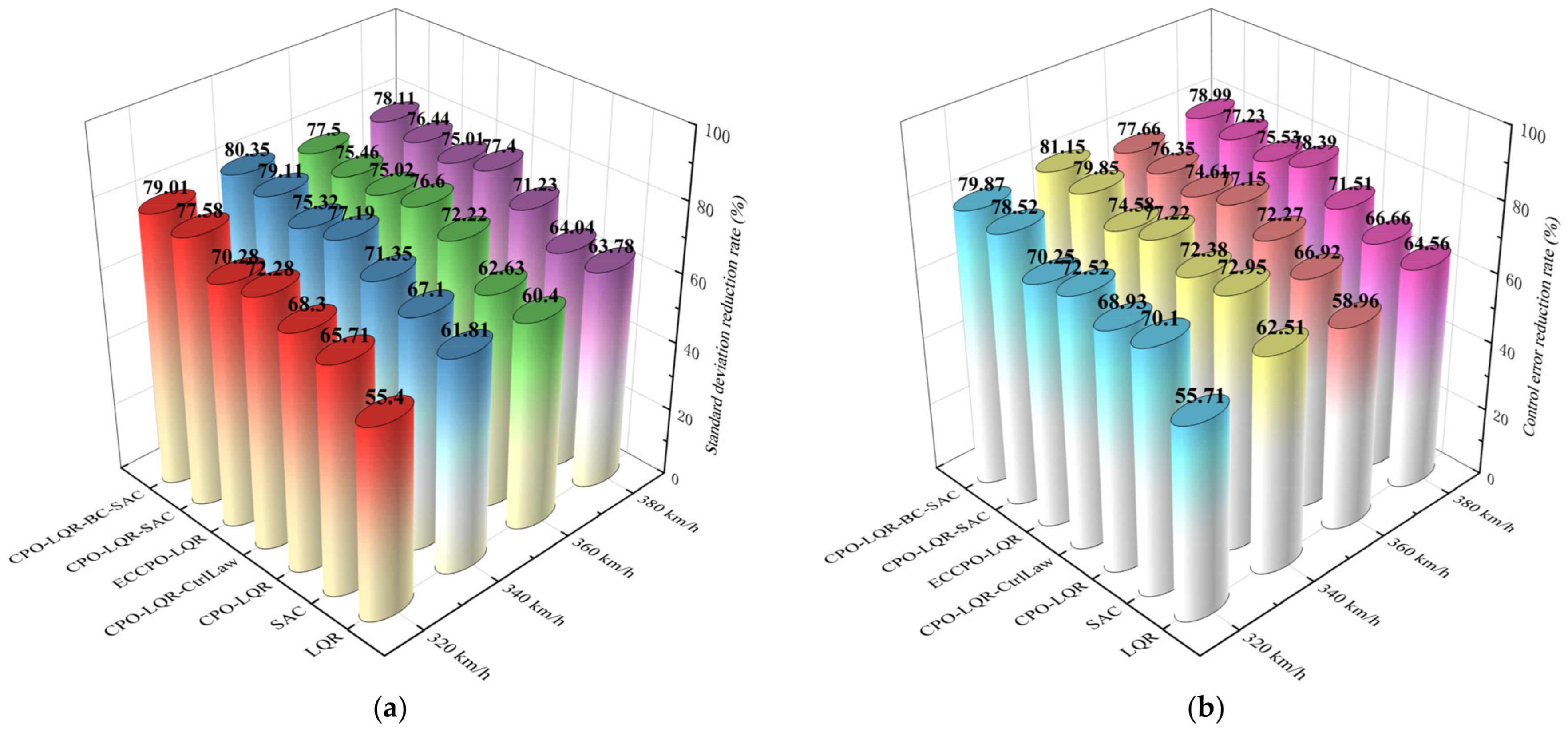
As observed in the table above, the proposed framework achieves the lowest standard deviation of contact force across all four speed conditions compared to the other control schemes, with the highest standard deviation reduction rates of 80.35%, and all the highest standard deviation reduction rates exceeding 77%. Concurrently, it also attains the minimum error mean while demonstrating comparably the highest error reduction rates of 81.15%, also exceeding 77% under all four speed conditions. These metrics substantiate the superior control performance of CPO-LQR-BC-SAC over other control architectures. Crucially, progressive performance enhancement is evident: transitioning from SAC to CPO-LQR-CtrlLaw and ultimately to CPO-LQR-BC-SAC control yields sequentially decreasing standard deviation values and monotonically increasing standard deviation reduction rates. This systematic improvement pattern, mirrored in error metrics, validates the gradient optimization paradigm embedded in our compensation framework design. For enhanced visualization of the control schemes’ performance across speed conditions, the tabular data is reconstituted in Figure 17.

As shown in Figure 17a, for standard deviation reduction across all speed conditions, the seven control schemes display an overall increasing trend in reduction rates, and our CPO-LQR-BC-SAC framework consistently achieves the highest values. Although the ideal dual-model offline control method CPO-LQR-CtrlLaw also performs strongly at all speeds (ranking second at 360 km/h and 380 km/h, and third at 320 km/h and 340 km/h), its reduction rate is always lower than that of the proposed framework. This not only verifies the effectiveness of offline tuning actions but also highlights the advantages of our proposed framework. From the control schemes’ perspective, the standard deviation reduction rate generally increases with speed; however, in the higher speed conditions (360–380 km/h), the gains for both CPO-LQR-BC-SAC and CPO-LQR-SAC taper off. This is likely due to more severe contact-force oscillations at higher speeds and the resulting instability in the agent’s exploration strategy, which limits further improvements—consistent with their reward convergence behavior. Fortunately, even in this speed band, our framework remains the top performer. The control error reduction shown in Figure 17b follows a similar pattern. Notably, SAC alone achieves error reduction rates of 70.10% and 72.95% at 320 km/h and 340 km/h—slightly above CPO-LQR’s 68.93% and 72.38%—but these gaps are minimal. At all other speeds, the improvement trends mirror those of the standard deviation reduction.

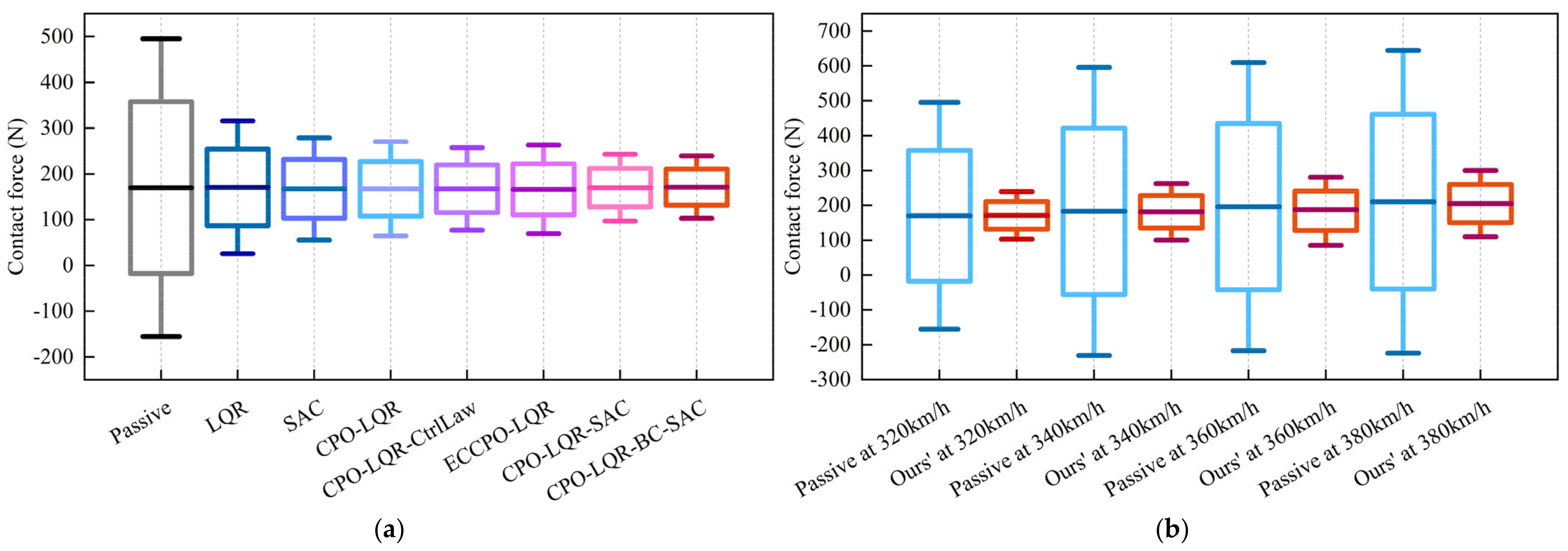
Based on the statistical contact force ranges discussed in Section 2.3.1, we compared the statistical distribution range of contact force under each control scheme at 320 km/h, as shown in Figure 18a. Similarly, we also compared the statistical contact force ranges under passive control and the proposed framework across all four speed conditions, as shown in Figure 18b. Whether examined by control scheme (Figure 18a) or by speed condition (Figure 18b), the statistical contact force ranges under the proposed framework consistently remain close to the target value, whereas in the passive control scenario, this range is markedly wider. These results further confirm the superior performance of the proposed compensation control framework in suppressing contact force fluctuations.

Furthermore, it is important to note that the adoption of LQR and SAC in the proposed framework is motivated by previous research findings. Specifically, LQR is included based on the results reported in [11], where it has been demonstrated to achieve highly effective control performance. Similarly, SAC is incorporated with reference to [17,18], which demonstrated that SAC outperforms other DRL-based control algorithms in exploring control actions for continuously oscillatory tasks such as pantograph–catenary contact force regulation. Therefore, LQR and SAC were selected as the core components for comparative evaluation in this study. To provide an approximate performance reference relative to the existing work, we extracted control performance metrics from two recent studies—CB-DMRL [18] and IDDPG [19]—which were conducted under comparable speed conditions (320–380 km/h). A summary of these results is presented in

Table 5. Comparison with existing advanced control algorithms at different speeds.

Speeds	Methods	${\mathit{\delta }}_{\mathit{S}\mathit{T}\mathit{D}}$	Pct. Decline
320 km/h	VFPID [19]	51.86	32.88%
	PH∞ [18]	35.64	7.38%
	PPO [18]	34.51	10.31%
	CB-DMRL [18]	32.82	14.71%
	IDDPG [19]	42.98	45.12%
	CPO-LQR-BC-SAC (ours)	22.77	79.01%
340 km/h	VFPID [19]	-	-
	PH∞ [18]	33.81	11.16%
	PPO [18]	32.94	13.47%
	CB-DMRL [18]	31.62	16.93%
	IDDPG [19]	-	-
	CPO-LQR-BC-SAC (ours)	27.08	80.35%
360 km/h	VFPID [19]	52.25	35.59%
	PH∞ [18]	42.83	12.41%
	PPO [18]	41.10	15.93%
	CB-DMRL [18]	38.52	21.22%
	IDDPG [19]	43.99	45.76%
	CPO-LQR-BC-SAC (ours)	30.98	77.50%
380 km/h	VFPID [19]	-	-
	PH∞ [18]	64.13	15.21%
	PPO [18]	57.94	23.40%
	CB-DMRL [18]	48.65	35.69%
	IDDPG [19]	-	-
	CPO-LQR-BC-SAC (ours)	31.68	78.11%

.

Although the exact simulation environments, and disturbance assumptions in those works differ from ours, a speed-matched comparison shows that our proposed CPO-LQR-BC-SAC framework achieves significantly lower contact force standard deviations and higher reduction rates across all test speeds. For instance, at 320 km/h, our method reduces the standard deviation to 22.77 N (79.01%), outperforming both CB-DMRL (32.82 N, 14.71%) and IDDPG (42.98 N, 45.12%). Similarly, at 380 km/h, our framework maintains a reduction rate of 78.11%, considerably higher than CB-DMRL’s 35.69%.

Since vehicle speed is the most critical factor affecting control performance, surpassing the impact of other disturbances in both simulations and real-world applications, we aligned the test conditions in terms of speed to ensure a fair comparison. Additionally, our work adopts modeling procedures based on the EN50318 [28] and GB/T 32591 [29] standards, ensuring consistency in the modeling framework. Although the experimental platforms are not entirely identical and some implementation details of the two referenced works are not fully disclosed, this comparison is not intended as a strict benchmark. Rather, it serves as a contextual reference that highlights the potential performance advantage of our method under similar speed conditions. Our approach consistently delivers better control performance at the same speeds, demonstrating both its effectiveness and its potential generalizability to practical applications.

4.4.2. Robustness Validation Across Different Pantograph Types

The control strategy trained using the parameters of the DSA380 pantograph was directly transferred to two different pantograph types—DSA350S and SSS400+—and tested in simulation at 320 km/h to evaluate whether the proposed framework can maintain its control performance under parameter variations. The model parameters of the two additional pantograph types are listed in

Table 6. Main parameters of the DSA350S and SSS400+ pantographs.

Parameters	DSA350S	SSS400+
$m_1$ (kg)	6.4	6.1
$m_2$ (kg)	7	10.2
$m_3$ (kg)	12	10.3
$k_1$ (N·m−1)	2650	10,400
$k_2$ (N·m−1)	10,000	10,600
$k_3$ (N·m−1)	0	0
$c_1$ (N·s·m−1)	100	10
$c_2$ (N·s·m−1)	100	0
$c_3$ (N·s·m−1)	70	120

.

As shown in Figure 19, even with changes in the model parameters, the proposed framework not only demonstrates significant superiority over passive control but also consistently outperforms the baseline CPO-LQR method, effectively suppressing contact force fluctuations. From both the contact force and error waveforms, it is evident that the oscillation amplitude is notably reduced for both pantograph types, and the errors are smaller than those under the baseline control. It should be noted, however, that although strong control performance is retained, a certain performance drop compared to the results on DSA380 is inevitable. To illustrate this difference more clearly, a cross-type comparison of performance metrics is presented in

Table 7. Comparison of control performance metrics across different pantograph types.

Types	Methods	${\mathit{\delta }}_{\mathit{S}\mathit{T}\mathit{D}}$	Pct. Decline
DSA380	Passive Control	108.47	-
	CPO-LQR	34.38	68.30%
	CPO-LQR-BC-SAC (ours)	22.77	79.01%
DSA350S	Passive Control	52.07	-
	CPO-LQR	25.70	50.65%
	CPO-LQR-BC-SAC (ours)	24.41	53.13%
SSS400+	Passive Control	108.56	-
	CPO-LQR	40.25	62.92%
	CPO-LQR-BC-SAC (ours)	38.27	64.74%

.

The results show that the standard deviation reduction rate is the lowest on DSA350S and slightly higher on SSS400+, both below the 79.01% reduction rate achieved on DSA380. The largest performance drop occurs on DSA350S, which is partly due to its already lower standard deviation under passive control, leaving less room for improvement. Nevertheless, the performance for both additional types remains in the high-performance range and surpasses that of the baseline CPO-LQR, indicating that the control strategy exhibits a certain degree of model robustness. This robustness stems from two main factors: (1) the baseline CPO-LQR controller inherently possesses robustness, and (2) the BC-SAC compensation strategy does not compromise system stability but instead enhances the suppression of fluctuations within a controlled range. Consequently, the proposed framework can maintain excellent control performance even under variations in pantograph model parameters.

5. Conclusions

This article addresses extreme PCCF fluctuations in high-speed railway systems by proposing a CPO-LQR-BC-SAC active compensation control framework, which progressively integrates optimization, imitation learning, and reinforcement learning to achieve high-performance suppression of contact force fluctuations. The main conclusions are as follows:

(1)

The baseline CPO-LQR controller is constructed and optimized using the CPO algorithm, yielding a high-performance control policy that effectively reduces PCCF fluctuations across varying speeds.

(2)

An offline secondary-tuned control law based on a dual-model structure further refines the control actions and provides expert demonstrations that enhance oscillation suppression.

(3)

A practical compensation strategy is developed by integrating real-time CPO-LQR outputs with expert action corrections within a unified single-model framework.

(4)

The CPO-LQR-BC-SAC learning framework is trained through a hybrid of behavior cloning and SAC, enabling it to imitate expert actions while maintaining exploratory capabilities.

The proposed framework reduces the standard deviation of PCCF by over 77% across all tested speeds and demonstrates the generalization capability to transfer the control strategy to different pantograph types. Future research will aim to enhance model fidelity by incorporating extreme-condition factors such as line tension variations, crosswinds, and structural heterogeneity. Furthermore, hardware-in-the-loop experiments will be conducted to validate the practical stability of the framework and support its real-world deployment.

References

1. Wu, G.; Dong, K.; Xu, Z. Pantograph–catenary electrical contact system of high-speed railways: Recent progress, challenges, and outlooks. Railway Eng. Sci. 2022, 30, 437–467. [Google Scholar] [CrossRef]
2. Daocharoenporn, S.; Mongkolwongrojn, M.; Kulkarni, S.; Shabana, A.A. Prediction of the pantograph/catenary wear using nonlinear multibody system dynamic algorithms. J. Tribol. 2019, 141, 051603. [Google Scholar] [CrossRef]
3. Karaduman, G.; Akin, E. A deep learning based method for detecting wear on the current collector strips’ surfaces of the pantograph in railways. IEEE Access 2020, 8, 183799–183812. [Google Scholar] [CrossRef]
4. Wu, Q.; Gu, X.P.; Ma, Z.; Wang, A. A study on the vibration characteristics and damage mechanism of pantograph strips in a railway electrification system. Machines 2022, 10, 710. [Google Scholar] [CrossRef]
5. Mariscotti, A. The electrical behaviour of railway pantograph arcs. Energies 2023, 16, 1465. [Google Scholar] [CrossRef]
6. Liu, Y.; Quan, W.; Lu, X.; Liu, X.; Gao, S.; Zhao, H.; Yu, L.; Zheng, J. A novel arcing detection model of pantograph–catenary for high-speed train in complex scenes. IEEE Trans. Instrum. Meas. 2023, 72, 5012013. [Google Scholar] [CrossRef]
7. Yu, X.; Wang, Z.; Song, M.; Song, L.; Yang, J.; Su, Y. Simulation study on arc temperature of urban rail DC pantograph–catenary and arc ablation of contact line. Machines 2024, 12, 514. [Google Scholar] [CrossRef]
8. Al-Awad, N.A.; Abboud, I.K.; Al-Rawi, M.F. Genetic algorithm–PID controller for model order reduction pantograph–catenary system. Appl. Comput. Sci. 2021, 17, 28–39. [Google Scholar] [CrossRef]
9. Farhan, M.F.; Shukor, N.S.A.; Ahmad, M.A.; Suid, M.H.; Ghazali, M.R.; Jusof, M.F. A simplified fuzzy logic controller design based safe experimentation dynamics for pantograph–catenary system. Indones. J. Electr. Eng. Comput. Sci. 2019, 14, 903–911. [Google Scholar] [CrossRef]
10. Song, Y.; Liu, Z.; Ouyang, H.; Wang, H.; Lu, X. Sliding mode control with PD sliding surface for high-speed railway pantograph-catenary contact force under strong stochastic wind field. Shock Vib. 2017, 2017, 4895321. [Google Scholar] [CrossRef]
11. Wang, B.; Wen, S.; Shen, Y. Active LQR control of a fractional-order pantograph–catenary system based on feedback linearization. Math. Probl. Eng. 2022, 2022, 2213697. [Google Scholar] [CrossRef]
12. Jin, X.; Lv, H.; Tao, Y.; Lu, J.; Lv, J.; Opinat Ikiela, N.V. Deep reinforcement learning-based active disturbance rejection control for trajectory tracking of autonomous ground electric vehicles. Machines 2025, 13, 523. [Google Scholar] [CrossRef]
13. Lin, Y.; Liu, X.; Zheng, Z. Discretionary lane-change decision and control via parameterized soft actor–critic for hybrid action space. Machines 2024, 12, 213. [Google Scholar] [CrossRef]
14. Gao, H.; Jiang, S.; Li, Z.; Wang, R.; Liu, Y.; Liu, J. A two-stage multi-agent deep reinforcement learning method for urban distribution network reconfiguration considering switch contribution. IEEE Trans. Power Syst. 2024, 39, 7064–7076. [Google Scholar] [CrossRef]
15. Liu, W.; Feng, Q.; Xiao, S.; Li, H. Automatic tracking control strategy of autonomous trains considering speed restrictions: Using the improved offline deep reinforcement learning method. IEEE Access 2024, 12, 75426–75441. [Google Scholar] [CrossRef]
16. Liu, W.; Feng, Q.; Li, H. Optimizing passengers’ experience: A goal-oriented reinforcement learning speed control approach for urban railway trains. Proc. Inst. Mech. Eng. Part F J. Rail Rapid Transit 2024, 238, 1283–1295. [Google Scholar] [CrossRef]
17. Wang, H.; Han, Z.; Liu, Z.; Wu, Y. Deep reinforcement learning based active pantograph control strategy in high-speed railway. IEEE Trans. Veh. Technol. 2022, 72, 227–238. [Google Scholar] [CrossRef]
18. Wang, H.; Liu, Z.; Han, Z.; Wu, Y.; Liu, D. Rapid adaptation for active pantograph control in high-speed railway via deep meta reinforcement learning. IEEE Trans. Cybern. 2023, 54, 2811–2823. [Google Scholar] [CrossRef]
19. Wang, Y.; Wang, Y.; Chen, X.; Wang, Y.; Chang, Z. An Improved Deep Deterministic Policy Gradient Pantograph Active Control Strategy for High-Speed Railways. Electronics 2024, 13, 3545. [Google Scholar] [CrossRef]
20. Sharma, R.; Mahajan, P.; Garg, R. Deep-reinforcement-learning-based controller design for pantograph and catenary system. Sādhanā 2025, 50, 46. [Google Scholar] [CrossRef]
21. Ambrósio, J.; Pombo, J.; Pereira, M. Optimization of high-speed railway pantographs for improving pantograph–catenary contact. Theor. Appl. Mech. Lett. 2013, 3, 013006. [Google Scholar] [CrossRef]
22. Bruni, S.; Ambrósio, J.; Carnicero, A.; Cho, Y.H.; Finner, L.; Ikeda, M.; Kwon, S.Y.; Massat, J.-P.; Stichel, S.; Tur, M.; et al. The results of the pantograph–catenary interaction benchmark. Veh. Syst. Dyn. 2015, 53, 412–435. [Google Scholar] [CrossRef]
23. Zhu, M.; Zhang, S.Y.; Jiang, J.Z.; Macdonald, J.; Neild, S.; Antunes, P.; Pombo, J.; Cullingford, S.; Askill, M.; Fielder, S. Enhancing pantograph–catenary dynamic performance using an inertia-integrated damping system. Veh. Syst. Dyn. 2022, 60, 1909–1932. [Google Scholar] [CrossRef]
24. Yu, W.; Li, J.; Yuan, J.; Ji, X. LQR controller design of active suspension based on genetic algorithm. In Proceedings of the 2021 IEEE 5th ITNEC, Xi’an, China, 25–27 June 2021; pp. 1056–1060. [Google Scholar] [CrossRef]
25. Tang, L.; Luo Ren, N.; Funkhouser, S. Semi-active suspension control with PSO-tuned LQR controller based on MR damper. Int. J. Automot. Mech. Eng. 2023, 20, 10512–10522. [Google Scholar] [CrossRef]
26. Wang, Y.; Li, H.; Meng, H.; Wang, Y. Dynamic characteristics of an underframe semi-active inerter-based suspended device for high-speed train based on LQR control. Bull. Pol. Acad. Sci. Tech. Sci. 2022, 70, 141722. [Google Scholar] [CrossRef]
27. Alfi, S.; Bruni, S.; Goodall, R.M.; Ward, C.P. Secondary yaw control to improve curving vs. stability trade-off for a railway vehicle. Veh. Syst. Dyn. 2022, 61, 1367–1386. [Google Scholar] [CrossRef]
28. EN50318; Railway Applications—Current Collection Systems—Validation of Simulation of the Dynamic Interaction Between Pantograph and Overhead Contact Line. European Committee for Electrotechnical Standardization: Brussels, Belgium, 2018; pp. 1–20.
29. GB/T 32591; Railway Applications—Current Collection Systems—Validation of Simulation of the Dynamic Interaction Between the Pantograph and the Overhead Contact Line. General Administration of Quality Supervision, Inspection and Quarantine of the People’s Republic of China, and the Standardization Administration of China: Beijing, China, 2016; pp. 1–10.
30. Guo, J.; Yang, S.; Gao, G. Research on active control of the pantograph–catenary system with varying stiffness (in Chinese). J. Vib. Shock. 2005, 24, 15–144. [Google Scholar] [CrossRef]
31. Song, Y.; Liu, Z.; Wang, H.; Lu, X.; Zhang, J. Nonlinear analysis of wind-induced vibration of high-speed railway catenary and its influence on pantograph–catenary interaction. Veh. Syst. Dyn. 2016, 54, 723–747. [Google Scholar] [CrossRef]
32. Song, Y.; Zhang, M.; Øiseth, O.; Rønnquist, A. Wind deflection analysis of railway catenary under crosswind based on nonlinear finite element model and wind tunnel test. Mech. Mach. Theory 2022, 168, 104608. [Google Scholar] [CrossRef]
33. Song, Y.; Ouyang, H.; Liu, Z.; Mei, G.; Wang, H.; Lu, X. Active control of contact force for high-speed railway pantograph–catenary based on multi-body pantograph model. Mech. Mach. Theory 2017, 115, 35–59. [Google Scholar] [CrossRef]
34. Zhou, H.; Liu, Z.; Xiong, J.; Duan, F. Characteristic analysis of pantograph–catenary detachment arc based on double-pantograph catenary dynamics in electrified railways. IET Electr. Syst. Transp. 2022, 12, 238–250. [Google Scholar] [CrossRef]
35. Abdel-Basset, M.; Mohamed, R.; Abouhawwash, M. Crested porcupine optimizer: A new nature-inspired metaheuristic. Knowl.- Based Syst. 2024, 284, 111257. [Google Scholar] [CrossRef]
36. Haarnoja, T.; Zhou, A.; Hartikainen, K.; Tucker, G.; Ha, S.; Tan, J.; Kumar, V.; Zhu, H.; Gupta, A.; Abbeel, P.; et al. Soft actor-critic algorithms and applications. arXiv 2018, arXiv:1812.05905. [Google Scholar] [CrossRef]
37. Torabi, F.; Warnell, G.; Stone, P. Behavioral cloning from observation. arXiv 2018, arXiv:1805.01954. [Google Scholar] [CrossRef]
Figure 1. Adverse contact phenomena caused by extreme contact forces during pantograph–catenary interaction.
Machines 13 00769 g001
Figure 2. Sketch of catenary system.
Machines 13 00769 g002
Figure 3. Three-mass pantograph model.
Machines 13 00769 g003
Figure 4. Schematic diagram of the interaction between the active control agent and the pantograph environment.
Machines 13 00769 g004
Figure 5. Target contact force values and the statistical contact force ranges under passive control for speeds from 300 km/h to 400 km/h.
Machines 13 00769 g005
Figure 6. Schematic of the core controller architecture and control system block diagram of the proposed active pantograph control strategy.
Machines 13 00769 g006
Figure 7. Flowchart for optimizing the Q -weight matrix weight coefficients using the CPO algorithm.
Machines 13 00769 g007
Figure 8. Conceptual basis for the design of the offline control law.
Machines 13 00769 g008
Figure 9. Schematic of the updated process for the active pantograph compensation control algorithm based on the CPO-LQR-BC-SAC framework.
Machines 13 00769 g009
Figure 10. Comparison of the fitness convergence for Q -matrix optimization between the CPO algorithm and classic methods under various speed conditions. (a) Under the 320 km/h operating condition. (b) Under the 340 km/h operating condition. (c) Under the 360 km/h operating condition. (d) Under the 380 km/h operating condition.
Machines 13 00769 g010
Figure 11. Comparison of the contact force fluctuation suppression under different speed conditions. (a) Under the 320 km/h operating condition. (b) Under the 340 km/h operating condition. (c) Under the 360 km/h operating condition. (d) Under the 380 km/h operating condition.
Machines 13 00769 g011
Figure 12. Effect of different increment values Δ u on the control performance of the control law.
Machines 13 00769 g012
Figure 13. Comparison of the contact force fluctuation suppression between the baseline control method and the secondary-tuned control law. (a) Under the 320 km/h operating condition. (b) Under the 340 km/h operating condition. (c) Under the 360 km/h operating condition. (d) Under the 380 km/h operating condition.
Machines 13 00769 g013
Figure 14. Comparison of reward convergence curves under different speed conditions. (a) Under the 320 km/h operating condition. (b) Under the 340 km/h operating condition. (c) Under the 360 km/h operating condition. (d) Under the 380 km/h operating condition.
Machines 13 00769 g014
Figure 15. Comparison of suppression performance on contact force based on the DRL method. (a) Contact force fluctuation and control error under the 320 km/h operating condition. (b) Contact force fluctuation and control error under the 340 km/h operating condition. (c) Contact force fluctuation and control error under the 360 km/h operating condition. (d) Contact force fluctuation and control error under the 380 km/h operating condition.
Machines 13 00769 g015aMachines 13 00769 g015b
Figure 16. Comparison of the proposed framework versus the expert action-based control schemes. (a) Contact force fluctuation and control error under the 320 km/h operating condition. (b) Contact force fluctuation and control error under the 340 km/h operating condition. (c) Contact force fluctuation and control error under the 360 km/h operating condition. (d) Contact force fluctuation and control error under the 380 km/h operating condition.
Machines 13 00769 g016
Figure 17. Control performance comparison of all the control schemes under various speed conditions. (a) Comparison of standard deviation reduction rates. (b) Comparison of control error reduction rates.
Machines 13 00769 g017
Figure 18. Comparison of post-control statistical contact force ranges: (a) Comparison of statistical contact force across different algorithms at 320 km/h; (b) Comparison of statistical contact force at different speeds under the proposed framework.
Machines 13 00769 g018
Figure 19. Test results of the control strategy on two different pantograph types. (a) Control performance when the strategy is transferred to the DSA350S pantograph. (b) Control performance when the strategy is transferred to the SSS400+ pantograph.
Machines 13 00769 g019aMachines 13 00769 g019b